
Abstract
Quantile regression (QR) provides an alternative to linear regression (LR) that allows for the estimation of relationships across the distribution of an outcome. However, as highlighted in recent research on the motherhood penalty across the wage distribution, different procedures for conditional and unconditional quantile regression (CQR, UQR) often result in divergent findings that are not always well understood. In light of such discrepancies, this paper reviews how to implement and interpret a range of LR, CQR, and UQR models with fixed effects. It also discusses the use of Quantile Treatment Effect (QTE) models as an alternative to overcome some of the limitations of CQR and UQR models. We then review how to interpret results in the presence of fixed effects based on a replication of Budig and Hodges’s work on the motherhood penalty using NLSY79 data.
Introduction
How does motherhood affect women’s earnings? This has been an important question for social scientists, as child-rearing is a large contributing factor for the gender earnings gap. The effects of motherhood on earnings are particularly hard to isolate because of selection biases, confounders, and unobserved factors. Not all women become mothers, and motherhood is associated with a range of other factors, many of which cannot be directly observed. Although the literature has converged around an estimate of a 5–8 percent motherhood penalty for each additional child, recent studies show that this penalty likely varies across a mother’s earnings distribution and by education levels (Avellar and Smock 2003; Budig and England 2001; Budig and Hodges 2010, 2014; England et al. 2016; Gangl and Ziefle 2009; Killewald and Bearak 2014; Waldfogel 1997). Discrepancies in findings are partially explained by the use of different methodologies that implicitly answer different sets of questions.
In light of these discrepancies, how should a researcher go about answering the question, how does motherhood affect women’s earnings? Or, more precisely, how do women’s earnings differ when comparing earnings distributions between mothers and nonmothers? Or, how does the female wage distribution change when more women become mothers?
Traditionally, linear regression (LR) analysis has been the conventional method for answering questions such as these among social scientists. Under the classical linear model assumptions (CLMA; i.e., linearity, random sampling, no perfect collinearity, zero conditional mean, homoscedasticity, and normality), linear regression provides the best unbiased estimator for the expected change in a dependent variable, y, associated with a unit change in the independent variable, x, and conditional on all other controls remaining constant (Wooldridge 2016). This is also known as the marginal or partial effect of x on y because all other factors that affect earnings (observed and unobserved) are assumed constant. Under the CLMA, the estimated change can even be interpreted as a causal effect x has on y. 1 Although the classical assumptions are often hard to meet in practice, even with some deviations from these, namely, under heteroscedasticity and nonnormality of errors, linear regression models provide unbiased estimates of the average effects for the relationship between x and y. 2 As a result, linear regression analysis is often the starting point in most quantitative analyses and much of what social scientists “know” has been built on studies focused on the so-called average person.
With the ever-growing availability of longitudinal or panel data, the use of linear models that control for one or more high dimensional fixed effects has increased. This is important as it allows researchers to control for otherwise unobserved heterogeneity, making causal interpretations more reasonable. 3 For the analysis of earnings and motherhood, for example, individual fixed effects control for unobserved time-constant characteristics, including factors like skill or desire to be a parent. Linear regression models allow for the inclusion of fixed effects by explicitly adding dummy variable sets in the model specification or partialling out the fixed effects before implementing the data analysis.
Even when accounting for individual-level fixed effects, however, LR does not necessarily provide the best estimator for summarizing the relationship between two variables in settings where assumptions of homoscedasticity and normality do not hold. 4 For example, studies often involve the analysis of skewed variables with many outliers. This is especially true for earnings, which often includes a small number of very high values. In these studies, the median, which is less influenced by outliers than the mean, potentially offers a better summary of the data. Furthermore, even if LR can still be used to identify average effects, it ignores any heterogeneity of the relationships of interest, leaving out important variation across the distribution of y, and masking potential inequalities within the data.
When the relationship between x and y differs at high and low levels of y, researchers might be more interested in understanding the heterogeneity of these relationships, in addition to the relationship at the mean and median. Researchers may, for example, be interested in analyzing how motherhood affects high or low earning women who are otherwise similar in observed characteristics; how the distribution of earnings would change if a larger share of the population had children; or how earnings of mothers and women without children at the top or bottom of the distribution compare. This type of analysis can be accomplished using quantile regression (QR) methods that analyze heterogeneous relationships between dependent and independent variables across the conditional or unconditional distribution of the dependent variable (Firpo 2007; Firpo, Fortin, and Lemieux 2009; Koenker and Bassett 1978).
Although quantile regression constitutes a powerful methodological tool that allows researchers to analyze effects beyond the mean and across an entire distribution, there are still misunderstandings regarding what quantile regression models do and how to interpret them. Most notable have been discussions about when to apply conditional quantile regression (CQR) versus unconditional quantile regression (UQR) models and how to interpret the results. This is especially true in settings that require the inclusion of individual fixed effects using longitudinal data.
QR models became part of the motherhood penalty debate through an exchange between Budig and Hodges (2010, 2014) and Killewald and Bearak (2014). In addition to estimating the effects of motherhood on women’s wages across the wage distribution, these papers had an added challenge of controlling for unobserved characteristics using individual fixed effects in their analyses. Budig and Hodges (2010) first used CQR to analyze the motherhood penalty across the distribution, adjusting for individual fixed effects, and finding larger penalties for mothers at the lower end of the wage distribution. Killewald and Bearak (2014) responded to this analysis by reestimating the models using UQR, finding the largest penalty for mothers at the middle of the distribution. Finally, responding again, Budig and Hodges (2014), reestimated their models using UQR and different specifications for fixed effects with results similar to their first set of models. More recently, England et al. (2016) incorporated UQR with updated data to examine how motherhood penalties vary across different combinations of skill and wage levels with slightly different findings.
These debates extend beyond sociology. For instance, in the developmental literature, Petscher and Logan (2014) attempted to provide an introduction to CQR, but inadvertently suggested misleading interpretations that were later addressed by Wenz (2019). Wenz (2019) distinguished between CQR and UQR and laid additional assumptions required for the type of interpretation usually given to these methodologies. In health economics, Borah and Basu (2013) also provided a discussion on the differences between CQR and UQR models, but misinterpreted Firpo et al. (2009) UQR methods with the Firpo (2007) estimation of quantile treatment effects (QTE). More recently, Borgen, Huapt, and Wiborg (2020) have also emphasized the need to address differences in estimating individual-level and population-level effects.
In light of these ongoing debates, this paper provides an accessible review to quantile regression models that incorporate fixed effects with an emphasis on application with social science data. Specifically, we discuss the estimation and interpretation of three types of quantile regression models, comparing them to the standard LR model and addressing the application of these models to longitudinal data. As an empirical example for our discussion, we provide a replication of Budig and Hodges (2014), using the alternative methods. 5 This allows us to contribute to broader discussions regarding the magnitude of the motherhood penalty on the wage distribution.
We begin with a brief description of LR and review its interpretation under the classical assumptions. We then review standard conditional quantile regression (CQR), introduced by Koenker and Bassett (1978), emphasizing the connections to the LR model and the assumptions required for its interpretation. Next, we discuss unconditional quantile regression (UQR), introduced by Firpo et al. (2009) as a special case of Recentered Influence Function (RIF) regressions. We then discuss the use of QTE models following the work of Firpo (2007) and Firpo and Pinto (2016), and expanding on the use of RIF regressions. QTE can be considered as a compromise between CQR and UQR that focuses on analyzing the distributional impact of a single binary variable on the outcome of interest, holding the distribution of other characteristics constant. Finally, we conclude with a guide of best practices for applying quantile regression models that should be useful to researchers with different levels of statistical expertise.
In addition to addressing the interpretation of different models for estimating the motherhood penalty across the earnings distribution, this paper offers several broad contributions to the literature on QR models. First, we provide a simple and straightforward comparison of the most common QR models, emphasizing the differences between CQR and UQR. We describe how each model is capable of answering different sets of questions, depending on the interests of the researcher, and how they relate to each other and standard LR.
Second, in discussing the estimation of QTE models, we suggest an alternative method for QR analysis that has received less attention in the literature. The QTE model is essentially a compromise between CQR and UQR models that allows researchers to examine differences across two distributions caused by a single variable of interest, based on the methodology proposed by Firpo (2007) and Firpo and Pinto (2016).
UQR models are able to identify the effect of marginal changes in the distribution of all controlled characteristics, x, on the unconditional distribution of the outcome, y. 6 However, they cannot provide estimates of changes in the distribution of y when considering large changes in the distribution of the independent variables, x (Rothe 2010), especially when the variable of interest is discrete. 7 In contrast, QTE models allow researchers to estimate and identify distributional effects considering a large change in the distribution of a single discrete characteristic while controlling for other factors.
Third, we focus on how to estimate and interpret UQR and QTE models in the presence of individual-level fixed effects, specifically with longitudinal data, using the newly developed Stata command rifhdreg (Rios-Avila 2020a), which simplifies all intermediate steps necessary for the estimation of UQR and QTE models. 8 We also contrast the analysis with CQR in the presence of individual-level fixed effects using the methodology proposed by Canay (2011). As shown in our empirical example of the motherhood penalty, examining within-person change over time through QR models has been a complicated endeavor with conflicting results. We further note how this debate is tied to issues over incorporating fixed effects into QR models and assessing relationships across a distribution over time.
While we often use language that makes causal interpretations of the motherhood, as well as other control variables, across all the models discussed here, it should be emphasized that the identification of causal effects is often difficult. Problems of endogeneity, sample selection, omitted variables, and model specification, among others, are also present when estimating quantile regression models. Many of these problems have yet to be addressed in the literature. Nevertheless, the discussion we provide should help to clarify the kind of effects one is able to estimate using quantile regression methodologies, under ideal scenarios. Furthermore, while emphasizing the interpretation of the effect motherhood on wages, the main variable of interest, we also provide some discussion on other factors for the sake of completeness, but those should be better interpreted as correlational, rather than causal effects.
Linear Regression (LR)
In order to understand what quantile regression does and the difference between conditional and unconditional partial effects, it is useful to first review what LR does, especially when using longitudinal or panel data. For example, assume that a researcher has access to panel data on earnings information for a fixed number of women (N) across time (T). The interest lies in analyzing the effect of motherhood, measured by the number of children (x) on earnings (y), while controlling for other observed characteristics, such as marital status, education, occupation, and work experience (z). With panel data, it is possible to differentiate between unobserved individual characteristics that are constant across time (


Under the CLMA the coefficients of this model can be estimated via OLS using two strategies (Wooldridge 2016). The traditional approach is to assume the unobserved effect
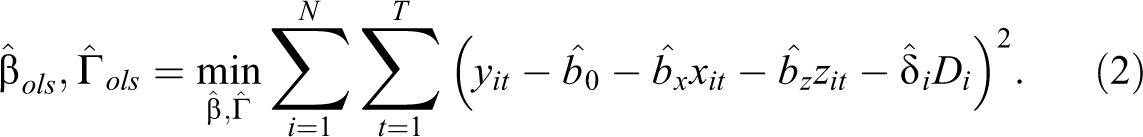
Because the parameters


Once the coefficients
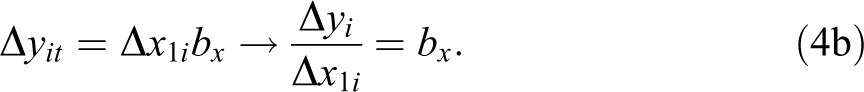
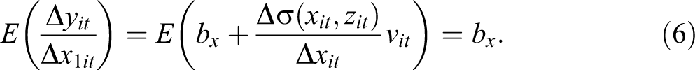
First, how much would the earnings for person i at time t change, if they had an additional child, keeping everything else constant? Under the assumption of homoscedasticity and using the model defined in equation (1a), this effect is equal to bx and constant across every woman:
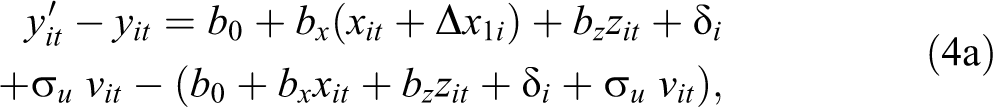
However, if the model is heteroskedastic with respect to number of children (x), this effect will not be constant (unobserved heterogeneity) and will depend on an unobserved component


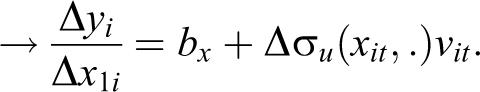
Because

Finally, it is also possible to make inferences for the population as a whole, by averaging the individual-level effect across all women in the sample. 13 This average effect would answer a third question: how much would average earnings in the population change if every woman had an additional child?
In summary, under the CLMA, there is no unobserved heterogeneity when estimating the individual, conditional, and unconditional levels effects. Because we assume a model that is linear in parameters and variables, the effect is constant regardless of individual characteristics.
14
If the model is heteroskedastic, the effects at the individual level will depend on unobserved factors. In this case, average effects conditional on characteristics and unconditional population average effects can still be used to abstract from the unobserved components and make inferences from the model. The presence of unobserved heterogeneous effects opens the possibility of analyzing the effects of changes in the independent variables across the distribution of the dependent variable,
Quantile Regression (QR)
QR models can be used to obtain a richer characterization of the relationships between independent and dependent variables that go beyond the mean. We review three QR methods that can be used for the analysis of effects across the conditional and unconditional distribution of
Conditional Quantile Regression (CQR)
Koenker and Bassett (1978) introduced conditional quantile regression into the econometrics toolbox over 40 years ago as an extension of the least absolute deviation estimator, which focuses on quantiles as a set of statistic that better describes the distribution of the outcome. Whereas LR models aim to explain how the expected outcome of a person changes in relation to a change in their characteristics, CQR tries to explain how the outcome of a person who is ranked above a specified quantile
Intuitively, this strategy takes advantage of the unobserved heterogeneity described in (4d), quantifying the size of the unobserved effect. In the context of our question, LR models can identify the average change in earnings if women with characteristics X and Z have an additional child (average effects conditional characteristics). In contrast, CQR can identify heterogeneous effects by quantifying changes in the distribution of earnings, measured in quantile differences, among women with characteristics X and Z if they were to have an additional child. 15 In other words, CQR can be used to answer the question—how does an additional child affect the conditional distribution of earnings, y, for a woman with observed characteristics X and Z?
To better understand the meaning of coefficients estimated through CQR, it is useful to start with the setup used for LR, explicitly lifting the homoscedasticity assumption, so that

In this setup, we can apply a quantile function


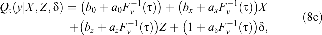

where
Although this setup is somewhat restrictive, it has implications that translate to the more general case of CQR.
16
First,
Third, the set of coefficients
Lastly, CQR cannot be used for individual level interpretations because effects at the individual level depend on an unknown factor,
When the model does not include individual fixed effects, for instance when using cross-sectional data, Koenker and Bassett (1978) show that the set of coefficients in this model
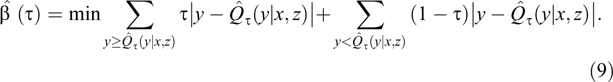
In contrast to the LR model, CQR cannot account for individual fixed effects by simply including sets of dummy variables representing each cross-sectional unit. Doing so creates an incidental parameter problem, affecting the consistent estimation of all coefficients in the model. 19 This problem has been discussed extensively in the literature (see Koenker 2004; Powell 2016; Canay 2011; and Machado and Santos Silva 2019), providing various procedures to obtain consistent estimates for other parameters of the CQR, under different assumptions. A simple approach for estimating conditional quantile regressions with fixed effects is discussed by Canay (2011).
As previously described, if the error Estimate the model Obtain

Although equation (10) can be directly estimated using the objective function described in equation (9), standard errors need to be estimated using other approaches such as bootstrap resampling methods. Assuming the true model is given by equation (7), CQR coefficients can also be estimated using the method of moments proposed by Machado and Santos Silva (2019). 20
The natural interpretation for CQR can be obtained by answering the question: how much would the earnings distribution change, measured by changes in the
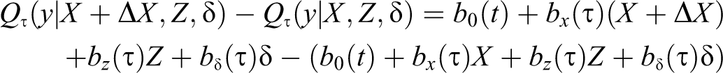

Three remarks are worth describing here. First, based on equation (11), we cannot make interpretations at the individual level because we do not know that person’s position in the conditional distribution (
Researchers, however, may be more interested in answering policy-related questions such as: how does motherhood affect the overall unconditional distribution of earnings? Or, how would the distribution of earnings change if every woman had an additional child? Answering this question requires a different type of analysis that incorporates the concept of unconditional quantile regression.
Unconditional Quantile Regression (UQR) based on the Recentered Influence Function (RIF)
As described in the previous section, the most important feature of CQR is its capacity to identify otherwise heterogeneous effects of changes in independent variables across conditional distributions. Often, however, researchers may be more interested in identifying the effects of changes of independent variables on the overall or unconditional distribution of the outcome. For example, instead of trying to identify how an additional child affects earnings for single mothers with one child, researchers may be interested in analyzing the effect of every woman in the population having an additional child on the unconditional distribution of earnings. In this sense, unconditional distributions are affected by changes in the distribution of other characteristics. There is, however, a close link between analyzing changes on conditional distributions and unconditional distributions.
Firpo et al. (2009) show that unconditional quantile effects 22 can be derived as a weighted average of all conditional quantile partial effects. Machado and Mata (2005) and Melly (2005) use a similar principle to simulate unconditional distributions of outcomes based on CQR to estimate unconditional quantile effects. In principle, the procedure requires the estimation of a large set of quantile regressions, for example, estimating separate models from the 1st through 99th conditional quantiles, to characterize the whole distribution of the dependent variable. After the models are estimated, simulation methods can be used to identify the effect of a change in the distribution of characteristics, for example, every woman having an additional child, on the distribution of the dependent variable. This process, however, is not always practical.
Addressing these impracticalities, Firpo et al. (2009) proposed a computationally simpler strategy to identify unconditional quantile effects that does not require reconstructing the entire distribution of the dependent variable. This methodology, unconditional quantile regression, uses the recentered influence function (RIF) to provide a first order approximation of the marginal effect of small location shift changes in the distribution of independent variables on any unconditional quantile. In practice, as described in Rios-Avila (2020a), this small shift changes should be understood as changes in the average of the independent variables.
In contrast with LR and CQR, RIF regressions in general, and UQR in particular, can only be used to draw inferences in terms of unconditional effects.
23
This implies that UQR can be used to analyze what would happen to the population
To better understand UQR, it is useful to understand what influence functions (IF) are, how they are constructed, and how they link to the unconditional distribution of the outcome. Assume women’s earnings (y) across time (t), is a random variable with cumulative distribution function Fy
and a density distribution

Assume there is a second distribution

Using these two distributions, the change in the distributional statistic caused by the added person is simply the difference between

This expression is also known as a directional or Gateaux derivative, and represents a first order (linear) approximation of the rate of change, or influence, an observation with earnings yi has on the distributional statistic v. To complement the idea of IF, Firpo et al. (2009) introduced the concept of the Recentered Influence Function, which is defined as:

In this case, the RIF is better understood as the linear approximation of the contribution of a single observation on the construction of the distributional statistic, v. The RIF has two important properties that have been discussed by von Mises (1947), Deville (1999), and Firpo et al. (2009):


The first property (16a) implies that the unconditional expectation of the RIF function is equal to the distributional statistic of interest. This property is the basis for interpreting RIF regression in the framework of unconditional effects. The second states that influence functions can be used to obtain the variance of distributional statistics v (Deville, 1999).
Although RIF functions can be used to analyze a large set of distributional statistics, 24 Firpo et al. (2009) concentrate on the analysis of unconditional quantiles, for which the RIF is defined as follows:

where
Once RIF’s have been obtained, UQR can be estimated through standard LR (RIF-OLS) using the corresponding RIF as the dependent variable, instead of y.
25
For instance, returning to the setup of panel data, where earnings (y) is a function of number of children (x), other explanatory variables (Z), individual fixed effect (

Even though quantile functions are inherently nonlinear, one of the main advantages of estimating UQR using OLS is that they can be easily adapted to include fixed effects, as discussed in Killewald and Bearak (2014) and Borgen (2016). In other words, it is possible to use the within transformation procedure described in section 2, to control for the individual effects
Three important aspects differentiate UQR from standard LR. First, equation (18) models how changes in the number of children relate to changes in the influence function person i has on the distributional statistic. The average of those changes can be interpreted as an effect on the unconditional quantile. Second, UQR has no interpretation in terms of individual or conditional effects. This happens because the RIF is constructed using the overall unconditional distribution, and thus can only be used to analyze influences on unconditional distribution statistics. 26 When using panel data, the unconditional distribution corresponds to the outcome distribution observed across all observations (individuals across time).
Third, because this strategy aims to analyze unconditional effects, all interpretations have to be made based on changes in the distribution of independent variables. If the model specification is set as in equation (18), without interactions or higher order polynomials, we assume that the only distributional changes of x that affect the unconditional quantile are changes in their means. 27
The natural interpretation of UQR can be obtained by answering the question: how much would the observed distribution of women’s earnings (across individuals and time) change, measured by the change in the


This partial effect is what Firpo et al. (2009) describe as the unconditional quantile partial effect, which is defined as the change in the unconditional quantile caused by a change in the distribution of x, approximated by a change in its mean value
When a variable is continuous with a wide range of values, using the thought experiment of “an additional unit change” is appropriate because such a change can be considered a “small” location shift effect, which UQR can approximate well. For example, an additional year of education is a small location shift compared to the average number of years of education in the population. However, an additional child likely results in a larger location shift, because a typical family has less than two children, and this may result in an incorrect interpretation of UQR estimates. In cases like this, instead of referring to one additional child per woman, one could refer to an increase in the fertility rate that results, for example, in a 0.2 increase in the average number of children.
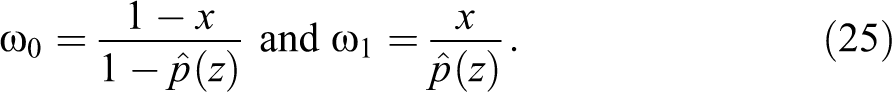
When the variable of interest is binary, for instance, being a mother (1) or not (0), the thought experiment described above is not adequate. On the one hand, only a fraction of the sample could change from “nonmothers” to “mothers.” On the other hand, comparing scenarios where every woman was a mother versus not would imply a large change in the distribution of motherhood, which UQR does not approximate well. Often, researchers incorrectly interpret coefficients of binary variables as if they were treatment effects, but they are not. A better interpretation is to treat the location shift as a change in the “incidence rate,” for example referring to a p percentage point increase in the share of mothers in the sample.
If a researcher is interested in analyzing distributional treatment effects, namely comparing the outcome distributions of two groups of individuals with the same distribution of characteristics, but who belong to different groups (e.g., treated and untreated group, mothers versus women without children), the most appropriate approach is to use a methodology known as quantile treatment effects.
Quantile Treatment Effects (QTE) via RIF
UQR models provide linear approximations of changes in how unconditional quantiles of the dependent variable change when there is a small change in the distribution of independent characteristics. Such approximations, however, may not be appropriate for analyzing large changes in the distribution of characteristics. This may happen when the characteristic of interest has a limited range of values (e.g., number of children), or when it is a binary variable (e.g., mothers and women without children).
When the variable of interest is binary, Firpo (2007) and Firpo and Pinto (2016) propose estimators that identify what they refer to as quantile or distributional treatment effects under the assumption of exogeneity. 28 These estimators use an inverse probability weights (IPW) to control for differences in the distribution of characteristics across two groups. Once such differences are controlled for, treatment effects of the variable interest are estimated by calculating differences in statistics across groups. The literature, however, is not clear regarding how to control for individual fixed effects when using this strategy.
Frölich and Melly (2010) present the command ivqte to implement the Firpo (2007) estimator. This command uses a semiparametric approach to estimate the IPW combined with a standard CQR procedure to identify quantile treatment effects. In contrast, the estimation procedure we propose relies on using RIF functions in combination with a probit or logit model for the estimation of the IPW weights, in the spirit of Firpo and Pinto (2016) and Firpo, Fortin, and Lemieux (2018). Using RIF function enables us to estimate a more flexible model that controls for differences in distribution of characteristics using the IPW, but also controls for them directly, by including them in the model specification, as it is done with UQR models.
Consider a situation where motherhood is measured as a binary variable

If we were able to observe both potential outcomes, quantile treatment effects could be estimated by calculating the differences in the

However, this is an unfeasible estimator. If the treatment motherhood were to be assigned at random, independent of all observed (z) and unobserved characteristics, quantile treatment effects could be estimated directly by calculating the difference in the

This is possible because, under the random assignment assumption, the observed distributions of earnings among the treated (or untreated) group


An alternative strategy to estimate the treatment effect is applying an extended use of RIF regressions. Specifically, rather than estimating equation (22c) via CQR, we can estimate this equation using RIF functions to approximate the conditional quantile of y. 29 Starting with equation (22b), we reorder the terms on the right side, and obtain:

Next, we obtain the RIF for equation (23), and use it as the dependent variable, in a regression similar to (22c) but that can be estimated using OLS:

According to Firpo (2007) and Firpo and Pinto (2016), if the treatment assignment is not random, even if it depends only on observed characteristics z (conditionally exogenous),
30
neither of the strategies above will correctly identify the treatment effects. This happens because the differences in quantiles captured by
Under the additional assumption that there are individuals with characteristics z among both the treated and untreated group (common support), Firpo (2007) and Firpo and Pinto (2016) suggest that distributional treatment effects can be identified using a two-stage procedure. In the first stage a set of weights are constructed to equalize the observed distribution of characteristics Z among the treated group and untreated groups. To do so, we first estimate a propensity score
In the second stage, the constructed weights are used to estimate the quantile average treatment effects using equation (22c) with a weighted quantile regression (Firpo 2007), or they can be used to construct the appropriate reweighted RIF functions and estimate equation (24) using weighted RIF regressions via OLS (Firpo et al. 2018). 31
In principle, IPW are used to reshape the observed distribution of characteristics z, so that the treated (or untreated) groups resemble the whole population. In doing so, the reweighted distribution of the observed outcome among the treated (or untreated) will be similar to the distribution of the potential outcome under treatment for the full sample. This estimation of the potential outcome distributions can then be used to identify the quantile treatment effects. 32 Despite the intuitive appeal of using these methods, IPW methods can be very sensitive when the propensity score is close to 0 or 1 (Lee, Lesser, and Stuart 2011). In such cases, the recommendation is to trim the weights, or propensity scores, in order to reduce the sensitivity of the estimates.
Unlike the CQR approach, the RIF regression approach (eq. 24) allows researchers to directly control for differences in the distribution of characteristics by including control variables in the model specification. This approach may be equivalent to the IPW regression adjustment estimator of the inequality treatment effects (Wooldridge 2010). In addition, it also allows researchers to obtain estimates for the covariates z that can be interpreted in the same way as variables in a UQR.
In contrast to other QR model estimation strategies, the literature has not yet reached a consensus regarding the estimation of fixed effects in the framework of QTE with panel data. 33 However, we suggest that it is feasible to use fixed effects as controls directly in the model specification making use of the properties of RIF-OLS regressions. Nevertheless, we concur that the estimation of QTE remains an open question when using panel data. Furthermore, when using panel data, like UQR, the QTE estimators compare distributions for the treated and untreated group pooling the information across years and individuals.
The interpretation of QTE estimations depends on whether the goal is to estimate average treatment effects or treatment effects on the treated (or untreated). For our example, if the treatment variable is motherhood, the interpretation can be obtained by answering the question: how much would the distribution of childless women’s earnings change, measured by the change in the
For other variables, the precise interpretation differs from UQR. Because the RIF is constructed for a distributional statistic conditional on x,
The proposed QTE estimator can be implemented with the Stata community-contributed command -rifhdreg- utilizing the option -over-, to define the treatment variable, and the options -rwprobit- or -rwlogit- for the estimation of propensity scores. It also provides the option -trim- to exclude observations with estimated propensity scores that are close to 0 or 1. This command also allows for the estimation of different treatment effects using the options att, ate, or atu, as described in Rios-Avila (2020a).
Application: Reexamining the Motherhood Penalty
Isolating the effects of motherhood on earnings has proven quite complicated for social scientists because it requires accounting for many confounding factors, some of which, such as work productivity and personal preferences, are hard to observe in survey data. Selection bias is also an issue, as only certain women may choose motherhood. As a result, researchers often rely on longitudinal data, most notably, the 1979 cohort of the National Longitudinal Survey of Youth (NLSY79), and fixed effects models to account for unobserved time-invariant individual-level factors in models that examine earnings over time. Results from these studies show that mothers experience an average wage penalty of 5–8 percent per child in the United States (Avellar and Smock 2003; Budig and England 2001; Gangl and Ziefle 2009; Waldfogel 1997). More recent work (Budig and Hodges 2010, 2014; England et al. 2016; Killewald and Bearak 2014) confirmed these findings, expanding the analysis beyond the mean, and indicating that the motherhood penalty varies across the wage distribution. However, due to the use of different QR models, these recent studies have led to conflicting findings regarding the motherhood penalty.
As illustrated by Budig and Hodges (2014), Killewald and Bearak (2014), and England et al. (2016), several issues arise when QR is used to analyze longitudinal data. First, the development of estimators for CQR with fixed effects is relatively new. None of the proposed methodologies has gained widespread usage because of the computational complexity of the method and the restrictive assumptions required for estimation. In contrast, because UQR can be estimated using OLS, this methodology can more easily account for fixed effects, which has gained attention in the applied literature.
Second, previous attempts to account for individual fixed effects were either computationally difficult to implement because they required a large number of parameters (dummy inclusion approach), or because they were not appropriate outside LR analysis (incidental parameter problem).
Third, the specific interpretation of the estimated effects depends on whether CQR or UQR is used, as these models capture conceptually different aspects of the relationships between dependent and independent variables. For instance, partial effects obtained using CQR are only valid when conditioning on all observed characteristics and cannot be easily generalized as effects on the unconditional distribution. On the other hand, partial effects obtained using UQR focus on explaining potential effects that may affect the distribution as a whole (the unconditional distribution), but they cannot be interpreted as effects for specific individuals. Additionally, because UQR relies on local approximations, the analysis of events like motherhood, may be biased if considered as a change that affects the motherhood status of all women in the sample.
In this section, we revisit Budig and Hodges (2010) to show how best to interpret findings related to the motherhood effect on earnings. To do so, we contrast insights from the LR model and the three types of quantile regression models discussed in Section 3, CQR, UQR and QTE, while accounting for individual fixed effects. We use the same model specifications and sample selection used in Budig and Hodges (2010; 2014). The sample contains 36,361 observations on 3,293 non-Hispanic white women, covering the years 1979–2004, extracted from the NLSY79. Following Budig and Hodges (2010), we examine the effect of number of children, as the proxy for motherhood, on logged hourly wages for women with wages between $1 and $200 per hour. The model specifications include sets of family structure, work effort, human capital, job characteristics, and demographic variables. 34
We assume that there are no issues involving endogeneity, self-selection, omitted variables, or incorrect model function forms, once individual fixed effects are accounted for. 35 We do this because we aim to replicate Budig and Hodges (2014), contrasting the findings across different methodologies. Furthermore, the specification is common across studies on the motherhood penalty. Nevertheless, it is important to consider that controlling for individual fixed effects only controls for time-fixed unobservable characteristics. If preferences for children change across time, using individual fixed effects may not be enough to control for those unobserved effects, which might generate inconsistent results. Because these assumptions are strong, causal interpretation is unrealistic in all cases. Nonetheless, they can be used as examples for the appropriate interpretation across different models.
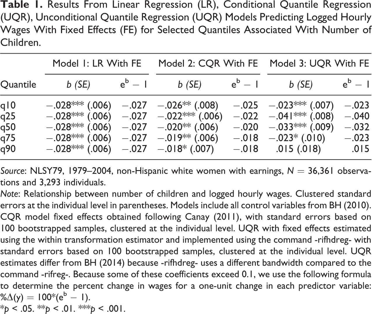
Given the differences between CQR and UQR with QTE models, we provide two sets of results. Table 1 provides estimates for the effect of the number of children on logged hourly wages across three model types with fixed effects—linear regression (Model 1, LR), conditional quantile regression (Model 2, CQR) and unconditional quantile regression (Model 3, UQR), while controlling for individual fixed effects. Table 2 uses the same models (Models 1–3) to show the effect of motherhood as a binary variable that takes the value of one if a woman has any children and incorporates quantile treatment effects (Model 4, QTE). Tables provide results from models that include all covariates and fixed effects. Additional model results are available in the Online Appendix, which can be found at http://smr.sagepub.com/supplemental/. Expanding on Tables 1 and 2, which provide estimates at the 10th, 25th, 50th, 75th, and 90th percentiles, Figures 1 and 2 present results from each model across the earnings distribution.
Results From Linear Regression (LR), Conditional Quantile Regression (UQR), Unconditional Quantile Regression (UQR) Models Predicting Logged Hourly Wages With Fixed Effects (FE) for Selected Quantiles Associated With Number of Children.
Source: NLSY79, 1979–2004, non-Hispanic white women with earnings, N = 36,361 observations and 3,293 individuals.
Note: Relationship between number of children and logged hourly wages. Clustered standard errors at the individual level in parentheses. Models include all control variables from BH (2010). CQR model fixed effects obtained following Canay (2011), with standard errors based on 100 bootstrapped samples, clustered at the individual level. UQR with fixed effects estimated using the within transformation estimator and implemented using the command -rifhdreg- with standard errors based on 100 bootstrapped samples, clustered at the individual level. UQR estimates differ from BH (2014) because -rifhdreg- uses a different bandwidth compared to the command -rifreg-. Because some of these coefficients exceed 0.1, we use the following formula to determine the percent change in wages for a one-unit change in each predictor variable: %Δ(y) = 100*(eb − 1).
*p < .05. **p < .01. ***p < .001.
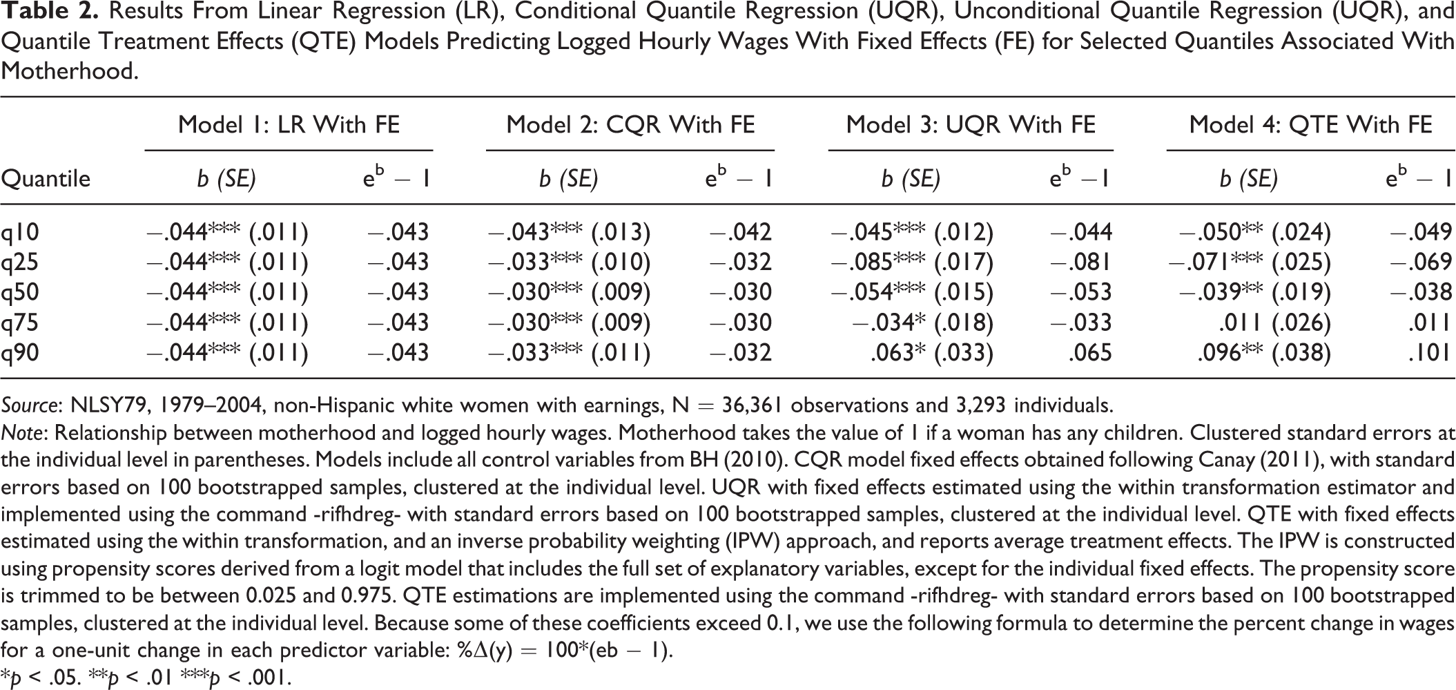
Results From Linear Regression (LR), Conditional Quantile Regression (UQR), Unconditional Quantile Regression (UQR), and Quantile Treatment Effects (QTE) Models Predicting Logged Hourly Wages With Fixed Effects (FE) for Selected Quantiles Associated With Motherhood.
Source: NLSY79, 1979–2004, non-Hispanic white women with earnings, N = 36,361 observations and 3,293 individuals.
Note: Relationship between motherhood and logged hourly wages. Motherhood takes the value of 1 if a woman has any children. Clustered standard errors at the individual level in parentheses. Models include all control variables from BH (2010). CQR model fixed effects obtained following Canay (2011), with standard errors based on 100 bootstrapped samples, clustered at the individual level. UQR with fixed effects estimated using the within transformation estimator and implemented using the command -rifhdreg- with standard errors based on 100 bootstrapped samples, clustered at the individual level. QTE with fixed effects estimated using the within transformation, and an inverse probability weighting (IPW) approach, and reports average treatment effects. The IPW is constructed using propensity scores derived from a logit model that includes the full set of explanatory variables, except for the individual fixed effects. The propensity score is trimmed to be between 0.025 and 0.975. QTE estimations are implemented using the command -rifhdreg- with standard errors based on 100 bootstrapped samples, clustered at the individual level. Because some of these coefficients exceed 0.1, we use the following formula to determine the percent change in wages for a one-unit change in each predictor variable: %Δ(y) = 100*(eb − 1).
*p < .05. **p < .01 ***p < .001.
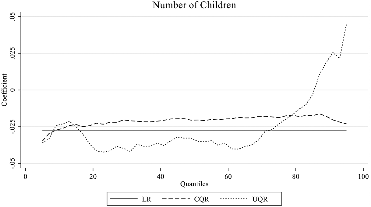
Partial effects of number of children on log wages: Comparison across LR, CQR and UQR. Source: NLSY79, 1979–2004, non-Hispanic white women with earnings, N = 36,361 observations and 3,293 individuals. Note: Results from linear regression (LR), conditional quantile regression (UQR), unconditional quantile regression (UQR) models include individual and year fixed effects (FE), and the full set of explanatory variables.
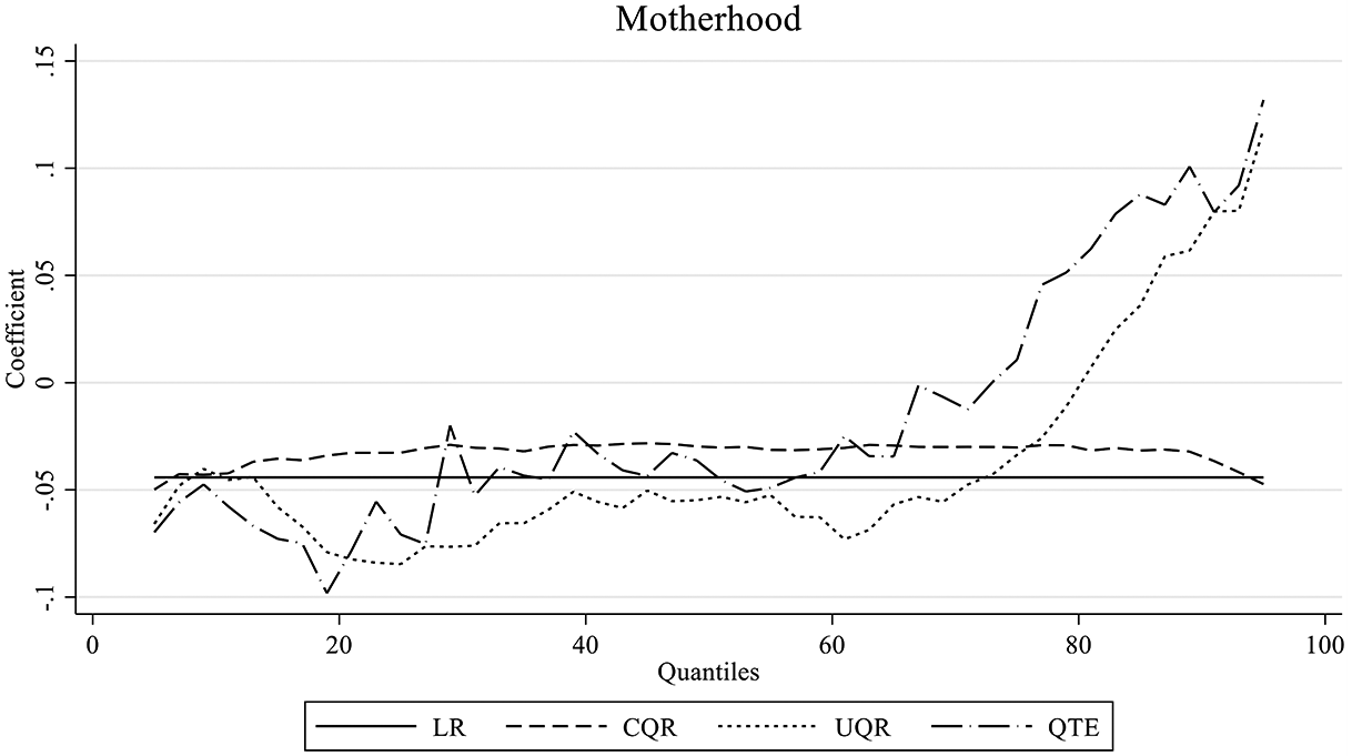
Partial effects of motherhood on log wages: Comparison across LR, CQR, UQR, and QTE. Source: NLSY79, 1979–2004, non-Hispanic white women with earnings, N = 36,361 observations and 3,293 individuals. Note: Results from linear regression (LR), conditional quantile regression (UQR), unconditional quantile regression (UQR), and quantile treatment effects (QTE) models include individual and year fixed effects (FE), and the full set of explanatory variables. QTE estimates correspond to the average treatment effects.
LR Estimates
According to the results in Model 1 in Table 1, there is a significant and negative wage penalty associated with motherhood, when measured as the discrete variable, number of children. Based on the LR model, mother’s wages are expected to decrease by 2.8 percent per additional child on average, a finding in line with Avellar and Smock (2003) and England et al. (2016) but lower than that of Budig and England (2001). 36 When measured as a binary variable (Table 2 Model 1), the effect of motherhood on wages is larger; it is associated with a wage reduction of about 4.3 percent. Although this is the most common way in which researchers interpret the estimated effects from LR models, we can also provide other interpretations to the partial effects dependent on certain model assumptions.
First, under the assumption of homoscedasticity, everyone in the population will experience the same effect. Consider, for example, three random women, one with no children, one with one child, and one with two children, the first model predicts each of these women will experience a decline in their wages of 2.8 percent if they had an additional child. 37 Alternatively, in the second model, upon becoming a mother, a woman would experience a wage decline of 4.3 percent. This interpretation can be considered the individual level partial effect.
Second, if we relax the assumption of homoscedasticity, we can no longer assume that every woman will experience the same effects associated with the birth of additional child. Consider all women who are identical in terms of their characteristics. For example, they are all 30 years old, married, and have one child, 12 years of education, 10 years of work experience, and so on. If they all have an additional child, each woman is not going to experience an identical wage penalty. Some will experience a larger decline in wages while others may experience no change at all. On average, however, having an additional child would reduce their wages by 2.8 percent. Alternatively, becoming a mother would reduce wages on average by 4.3 percent. This interpretation can be considered the conditional partial effect.
Finally, because the LR model specification assumes a linear relationship between the dependent and independent variables, we can also make inferences regarding the unconditional changes in wages across the population. For example, if every woman in the population has an additional child, assuming other characteristics remain constant, we would expect average wages among all women to decline by 2.8 percent. In this situation, it may be more accurate to discuss this effect in relation to a smaller change in the average number of children. For instance, if the average number of children increased by 0.5, we would expect average wages to decrease by 1.4 percent (2.8 percent × 0.5). This gives us the unconditional partial effect. In the case of motherhood, the interpretation refers to how much lower women’s wages would be if all women were mothers, compared to if they had no children. A more reasonable interpretation would indicate that if the share of mothers in the sample increased by 10 percent, average wages would decline in 0.43 percent.
The differences between interpreting LR results as individual, conditional, or unconditional partial effects are very fine distinctions that few studies make. This is understandable because such distinctions are not always central to most LR analyses. In fact, under the homoscedasticity assumption, no distinction is needed, because everyone in the population is affected in the same way. As this paper shows, however, understanding the differences between individual, conditional, and unconditional partial effects is crucial for interpreting results from conditional and unconditional quantile regression models.
CQR Estimates
Depending on the research question of interest, LR estimates can be used to draw inferences about how changes in the independent variables translate into changes in the dependent variable at the individual level (individual effect), on average for individuals with the same characteristics (conditional effects), or on the whole population average (unconditional effects). In the case of conditional quantile regression only the conditional effect interpretation is feasible for all independent variables, unless stronger assumptions regarding ranking are applied.
Model 2 in Tables 1 and 2 provides estimates of the motherhood penalty measured as number of children (Table 1) and as any children (Table 2) applying CQR with fixed effects using the Canay (2011) estimator. 38 Figures 1 and 2 also provide an illustration of the effects across the different quantiles. According to the CQR model results, motherhood has varying effects on earnings across the wage distribution. As shown with the LR results in Model 1, a typical woman experiences an average wage penalty of 2.8 percent per additional child and a 4.3 percent average wage penalty for being a mother and this is true at every quantile. Based on the CQR estimates in Model 2 (Table 1), however, a typical woman would experience a wage penalty that ranges between 2.6 percent if she is ranked at the 10th percentile to 1.8 percent if she is ranked at the 90th percentile, assuming her rank remain constant. The trend of the impact of motherhood (Table 2 Model 2), provides qualitatively similar results, suggesting that a typical woman may experience a larger wage penalty at the 10th percentile (4.2 percent), but a smaller penalty near the 90th percentile of the distribution (3.2 percent). Similar to Budig and Hodges’s (2010) CQR models, Figures 1 and 2 suggest that the motherhood penalty is larger for women at the bottom of the conditional distribution, although differences across the distribution are small.
We use the term “typical” woman to refer to a nonspecific woman who has average or median characteristics, thus stating the conditionality of the effects. This woman would be unmarried with no children and 12 years of education (approximately a high school diploma). We are also interpreting the coefficients under two strict assumptions. We assume that we know a specific woman’s position among other women with identical observed characteristics, and we assume that her position does not change after she has a new child (rank invariance assumption). Although both assumptions are consistent with the model as described in equation (8d), population rankings are never observed in empirical settings and the assumption that a person’s conditional ranking does not change is strong. This implies that we cannot make inferences for a specific individual because we do not know their ranking in the conditional distribution or if that ranking will remain constant after a change in the number of children.
A second interpretation, which is more fitting in the framework of CQR, refers to the conditional effect, implicitly acknowledging that we cannot be certain about individuals’ rankings. This can be accomplished in two ways. The first avoids references to specific individuals, and refers instead to groups of women who have the same characteristics. For example, we could say, if women with average characteristics had an additional child, their wage distribution would decline between 2.5 percent at the 10th percentile that declines to about 1.8 percent at the 90th percentile (Table 1 Model 2). Or, if the focus in on motherhood, the wage penalty after transitioning to motherhood would range from 4.2 percent at the 10th percentile to 3.2 percent at the 90th percentile (Table 2 Model 2).
An alternative way to understand the results is to consider the distribution of wages across two groups of women who are identical in every way except that one group comprises mothers with one child and the other comprises women with no children. The difference in average wages would be 2.8 percent for women with one additional child, according to the LR model. However, based on the CQR model, we should expect wages among women with one child at the 10th percentile to be 2.5 percent lower than wages for women without children, but only 1.8 percent lower at the 90th percentile (Table 1 Model 2). We would also expect wages among all mothers at the 10th percentile to be 4.2 percent lower than wages for women without children, but only 3.2 percent lower at the 90th percentile (Table 2 Model 2). This interpretation emphasizes how the two distributions compare to each other.
UQR Estimates
Model 3 in Tables 1 and 2 provides UQR results for selected quantiles for the effect of number of children and motherhood. In contrast to CQR, UQR models analyze how changes in the distribution of characteristics affect the unconditional distribution of the outcome, but these models do not provide information about how those changes influence individual experiences. This means that coefficients from UQR models must be interpreted in relation to how changes in the average number of children per woman or in the share of mothers affect the overall (across time) earnings distribution.
According to the LR results in Table 1 Model 1, if the average number of children per woman were to increase by one child between 1979 and 2004, average wages among all women would have been 2.8 percent lower. However, looking at the effects throughout the distribution, the UQR results in Model 3 suggest that a change in the distribution of the number of children will have a heterogeneous impact across the distribution of wages. If the average number of children per woman was to increase by one, we would expect wages at the bottom of the distribution to decrease by 2.3 percent, but we would also observe an increase in wages at the top of the distribution (90th percentile) by approximately 1.5 percent, although this last coefficient is not statistically significant. Figure 1 further illustrates this relationship. Although an increase in the average number of children per woman is negatively associated with wages for most of the distribution, the negative effect shrinks above the 60th percentile, turning positive and increasing around the 90th percentile.
When measured as a binary variable, the results in Table 2 Model 3 suggest a similar trend in terms of the wage penalty of motherhood, with an estimated impact that is positive and statistically significant at the top of the wage distribution. However, the most appropriate way to interpret the coefficients associated with motherhood relies on describing the effect associated with a marginal increase in the share of mothers in the sample. Based on the UQR results, if the share of mothers in the sample were to increase by 10 percentage points, wages at the bottom of the distribution would decrease faster than wages at the top. For instance, we would expect the 10th quantile of wages to decrease by 0.44 percent, the 50th quantile to decrease 0.53 percent. The results in Figure 2 suggests that above the 60th percentile, the negative effect of motherhood shrinks, with a positive impact above the 80th percentile. At the 90th percentile a 10 percentage point increase in the share of mothers may increase wages by 0.65%.
As indicated by our discussion, the interpretation of UQR results should be kept in terms of unconditional statistics. It is also important to consider that, in contrast with conditional effects, unconditional quantile effects are not isolated. For example, if each woman were to have an additional child, this would cause a change in earnings distribution that would be observed across all quantiles simultaneously. Because of this, plotting coefficients may be useful to appreciate the full extent of the distributional changes. Furthermore, while we use the language of “an additional child” effect, this may not be adequate because less than 10% of women in the sample have more than 3 children. This kind of interpretation is more appropriate when considering the motherhood as a binary variable. As the proportion of mothers in the sample increases, the whole distribution shifts, affecting all quantiles simultaneously.
QTE Estimates
Expanding on these more common models, Model 4 in Table 2 provides the QTE results for selected quantiles and at the mean. This model controls for differences in characteristics using IPW and includes these controls and individual fixed effects in the model specification. The IPW are constructed by trimming the propensity score to be between 0.025 and 0.975.
We again measure the effect of motherhood using a binary variable that takes the value of one if a woman has any children and zero otherwise. For the estimation of the QTE, a logit model is used for the estimation of the propensity score using the same variables used in Budig and Hodges’s (2010), except for the individual fixed effects. To reduce the sensitivity of the estimations to extreme propensity scores, the QTE are estimated excluding observations with a predicted propensity score below 0.025 and above 0.975. For comparison, we report average treatment effects (ATE), with ATE on the mean being reported in the Online Appendix, which can be found at http://smr.sagepub.com/supplemental/.
The estimated coefficients should be interpreted as the impact motherhood would have on the distribution of wages of all women, assuming that the distribution of other characteristics remain constant. In other words, the estimated effects measure how different the distribution of wages would be if we were to compare the wage distribution assuming all women are mothers, against all women not being mothers.
When controlling for observed covariates as part of the IPW and directly in the model specification and unobserved time-invariant characteristics using individual fixed effects in QTE models (Table 2 Model 4), we observe a trend in the average QTE similar to the one observed for the UQR (Table 2 Model 3). Based on these estimates, motherhood would have an heterogenous effect on the wage distribution, potentially reducing wages at the bottom of the distribution in as much as 5 percent at the 10th percentile and reducing wages by 3.8 percent in the middle of the distribution, but increasing wages at the 90th percentile by 10.1 percent. This average effect is larger than the effect estimated using UQR.
Importantly, QTE models should be interpreted by comparing the potential wages if all women were not mothers to a scenario where all women are mothers, and assuming the distribution of other characteristics remaining constant. While not discussed in this example, a researcher may also choose to interpret the average treatment effects on the treated (or untreated). This could facilitate the interpretation by analyzing potential effects on the treated or untreated group, rather than on the population as a whole.
Discussion
What is the relationship between x and y? Because social scientists typically use LR to answer this question, most research presents an answer and interpretation related to the mean that people have come to expect. This is a good example of how the methods we use to answer a research question shape the answers we find. Due to the ubiquity of linear regression models, much of the accumulated quantitative social science knowledge is based on the mean, which is not necessarily problematic. Often, the mean presents a good summary of the outcome, and, hence, a good description of the relationship between two variables, x and y. But, in many situations, when the relationship between x and y varies across the distribution of y, the mean might not offer the best summary available. Focusing on only the mean can obscure results, especially when researchers are interested in issues like gender inequality (Bernhardt, Morris, and Handcock 1995). When this happens, researchers must expand their toolkits to test new methods for studying this relationship.
Quantile regression provides a framework for analyzing heterogeneous effects beyond what LR can provide. However, in applying quantile regression, researchers must take care in defining a research question and interpreting the results. This comes down to determining what it means to ask and answer the questions—How does a change in x affect the outcome y for any individual in the data? How does a change in x affect the conditional distribution of y? Or, how does a change in x affect the unconditional distribution of y? Although QR models do not provide an answer to the first question like LR models do, CQR can be used to answer the second question, and UQR can be used to answer the third. In this paper, we also discuss a fourth strategy, QTE, as a middle ground between what CQR and UQR can estimate. This strategy answers the second question, with respect to a single variable of interest, by identifying a distributional treatment effect. Using RIF regressions to identify QTE, also allows a researcher to answer the third question for other variables in the model. Each method, therefore, provides a slightly different interpretation for the relationship between x and y across the distribution of y.
CQR can be used to study the relationship between variables across the conditional distribution of the outcome variable. However, the interpretation should be framed as effects experienced by groups that are defined by a set of characteristics (conditional effects). CQR models are easy to interpret in the case of a single variable, but interpretation problems typically arise once additional covariates are added. These controls essentially change an observation’s place in the distribution, implicitly creating subgroups defined by covariates. Because of this, the interpretation of the estimations should be considered as local effects, given a set of individuals with specific characteristics (e.g., women with the same years of education, hours of work, and marital status). These results cannot be generalized as effects that would affect the unconditional statistic of interest.
Overcoming this limitation, UQR provides an additional framework for analyzing heterogeneous effects across a distribution where the definitions of quantiles are not affected by individual values of model covariates, as they describe a characteristic of the distribution of y as a whole. However, because of this, UQR can only be used to identify effects on the unconditional distribution of the outcome. Consequently, coefficients can only be interpreted as in relation to how changes in the distribution of independent characteristics x, usually approximated by changes in the unconditional mean, affect the unconditional quantile of the outcome. Importantly, inferences are only valid when analyzing small changes in the distribution. Because of this, special care is needed when interpreting the effects of categorical and discrete data, such as motherhood and the number of children. UQR may not provide consistent estimates when the changes in the distribution of characteristics are large. Furthermore, it remains to the researcher to evaluate if the unconditional distribution, in a panel data framework, is appropriate for their research question.
QTE presents an important compromise between CQR and UQR. By constructing the RIF’s across groups defined by a single variable of interest, distributional treatment effects, measured via changes in quantiles, can be estimated and discussed. This allows researchers to examine how the distribution of the dependent variable, y, changes as the main conditioning variable changes, after controlling for differences in the distribution of other characteristics. If the model is estimated using RIF regressions, the interpretation of all other variables in the model is similar to the one for UQR. The interpretation of QTE will also depend on whether the researcher is interested in analyzing average treatment effects that apply to the population as a whole or treatment effects on the treated or untreated groups. Similar to UQR, it needs to be evaluated if unconditional distributions pooling data across time are of interest in a given research question.
What does this mean for the debate over using QR models to research the motherhood penalty? In this case, the use of different methods has led to varying results for the effects of children on women’s wages and a large debate over the “true” penalty of motherhood. Our replication of Budig and Hodges (2010) shows that neither type of QR model specification is essentially “right” or “wrong.” Each, however, offers a different interpretation and understanding of the motherhood penalty, as indicated in Tables 1 and 2, and Figures 1 and 2.
According to the LR model, controlling for time-varying covariates and unobserved individual-level time-invariant factors, there is a wage penalty associated with motherhood. Specifically, this model indicates that on average, having an additional child will reduce women’s wages by 2.8 percent, and if the average number of children per woman in the population increases by one, holding all other characteristics constant, women’s wages will decline by 2.8 percent. Using a different definition of motherhood, a binary variable, also suggests a larger effect of a 4.3 percent average penalty associated with motherhood. Certain QR models, however, indicate that this relationship varies across the conditional and unconditional wage distribution.
Estimates from the CQR model suggest that an additional child, or motherhood more generally, has a mostly homogenous effect for women across the conditional distribution. The CQR estimates also present a somewhat smaller wage penalty, predicting that among women with the same characteristics an additional child would lead to a wage decline of about 1.8–2.6 percent with larger penalties below the 50th percentile, and a wage decline of 3.2–4.2 percent when using the binary definition of motherhood.
Although having an additional child has a relatively stable negative effect on wages across the conditional wage distribution, the UQR results suggest a generalized increase in the number of children per woman in the population will have a more heterogenous impact on the unconditional distribution of wages observed across all years. If the average number of children per woman were to increase by one, the UQR estimates suggest that up to the 60th quantile, unconditional quantiles of wages would decline between 2.3 percent to 4.0 percent. For the upper section of the distribution, the decline shrinks to zero, and even small increases above the 85th quantile are estimated. Although the point estimates when using a binary definition of motherhood are larger when using UQR, the interpretation of the coefficients need to be rescaled to consider a marginal increase in the share of mothers in the sample.
Overall, the UQR results suggest that an exogenous increase in the number of children, or an increase in the share of mothers in the sample, will increase inequality, widening the wage gap between the top and the bottom of the distribution. However, this result should be considered cautiously for two reasons. First, because we are using panel data, UQR is measuring the impact of an additional child on the overall distribution of wages observed across all the survey waves. It is up to the researcher to decide the merits of analyzing changes on the overall wage distribution across multiple years. Second, half of the person-years in the sample have no children, and only 6 percent of those who are mothers have more than three children, thus the thought experiment of one additional child per women may not be appropriate in the context of UQR. Similar concerns are raised if we try to analyze the binary variable of motherhood as a treatment effect in the context of UQR.
In addition to replicating findings regarding a key question in the sociological literature, this paper incorporates an additional model based on quantile treatment effects that provides researchers with an alternative to CQR and UQR models. Based on our estimates, QTE, which aims to compare the distribution of women’s earnings based on their motherhood status, presents a varying relationship across the distribution, from a negative effect at the bottom, to a large and positive effect at the top of the distribution (up to 10 percent effect). These are similar to the point estimations obtained using the UQR model. Similar to the UQR analysis, however, it is up to the researcher to decide if analyzing a treatment effect on the overall distribution of wages across years is appropriate for their research question.
Results further support Budig and Hodges (2010, 2014) who found that mothers at the top of the wage distribution do not experience a motherhood penalty after controlling for key job characteristics, especially a change in work hours. In terms of mechanisms behind this relationship, it is important to note that women with wages this high have access to support in the form of nannies, chefs, and cleaning services that other women do not. The large wage premiums we find at the top of the wage distribution also suggest that there may be other factors, like individual time varying variables, we are not controlling for, that may be driving this effect. For instance, it is possible that women’s preferences for having children may change over time.
Conclusion
With several potential models, what’s a researcher who wants to study the relationship between x and y across the distribution of y to do? Thankfully, there are several options for approaching this problem through quantile regression. Below, we list a set of best practices for applying quantile regression models. These best practices are not exhaustive, but they do provide a roadmap toward approaching a study that requires QR analysis. Most suggestions also relate to steps that come before data analysis—an extremely important part of creating a research project that can often go overlooked.
Best Practices for QR
1. Clearly identify the research question and variables of interest.
As in any research article, the choice of the econometric approach will depend on the research question and relationship of interest. It is useful to remember that QR allows identifying heterogeneous effects with respect to the conditional (CQR) and unconditional distributions (UQR) of the dependent variable. QTE can be used if the interest lies on analyzing distributional treatment effects. If the interest lies in analyzing heterogeneity with respect to an independent variable, other approaches not discussed here may be required.
“How does motherhood affect women’s earnings?” is a broad question that can be answered in many ways. Perhaps the simplest answer comes from linear regression, which shows that, on average, each additional child is associated with a 2.8 percent decrease in women’s earnings and motherhood more generally is associated with a 4.3 percent decrease. However, that still leaves open questions of heterogeneity. Is the motherhood penalty larger for low-wage or high-wage women? Asking this question creates a need to examine the relationship between motherhood and earnings across the wage distribution, but it can be answered in multiple ways that examine either the conditional or unconditional wage distributions. Here, it is important to identify if the interest falls in analyzing the effects that any particular woman will experience or if the interest falls in analyzing how changes in the overall number of children in the population or motherhood status. In the case of the former, LR and CQR models are more appropriate, while UQR and QTE present better approaches for the latter. 2. Determine the most useful or adequate interpretation for answering the research question, especially in terms of interpreting partial effects.
As discussed from the beginning of this paper, LR provides a good approximation of the average effects between dependent and independent variables that is applicable for most research questions. If the interest lies in analyzing heterogeneous effects, CQR can be used to analyze local effects of how changes in an independent variable affect the conditional distribution of the dependent variable, which complement the average effects identified using LR. If the interest lies in analyzing global distribution effects, UQR can be used to identify how small changes in the distribution of independent variables affect the distribution of the dependent variable, measured by changes in the unconditional quantiles. Finally, if the interest lies in analyzing distributional effects of policies or large changes in the independent variables, thus analyzing how two or more distributions compare across quantiles, after controlling for the distribution of other factors, QTE may be the most appropriate approach.
In the case of the motherhood penalty, CQR model results indicate that wages among mothers at the 10th percentile would be 4.2 percent lower than wages for women without children, but only 3.2 percent lower at the 90th percentile (Table 2 Model 2). UQR results indicate that if the share of mothers in the sample were to increase by 10 percentage points, the 10th quantile of wages would decrease by 0.44 percent and the 50th quantile would decrease by 0.53 percent, but a 10 percentage point increase in the share of mothers at the 90th percentile may increase wages by 0.65 percent (Table 2 Model 3). Finally, QTE models indicate that if all women became mothers, this would decrease wages at the bottom of the distribution by 4.9 percent at the 10th percentile and 3.8 percent in the middle of the distribution, but increase wages at the 90th percentile by 10.1 percent (Table 2 Model 4). 3. Note the assumptions for the interpretations of different QR model types.
As described earlier, each QR model has its own advantages and limitations. While CQR can be used to estimate local effects in the distribution caused by changes in a single the independent variables, the effects cannot be described as an individual effect, unless rank invariance is assumed, nor extrapolated as an effect on the overall/unconditional distribution. UQR, on the other hand, can be used to draw global distributional effects caused by small changes in the distribution of characteristics, but cannot be used to draw inferences of individual or local effects. QTE, when estimated via RIF regressions, is a compromise between CQR and UQR. It allows us to estimate unconditional like effects for all characteristics except for a single conditioning variable for which a distributional treatment effects are obtained. 4. Compare results across multiple model types.
Although it is important to choose a method that best fits your research question, it is equally important to understand that all these methodologies complement each other, as they identify different aspects regarding the relationships between dependent and independent variables. Observing how results vary with a different model and interpretation may reveal patterns that are otherwise overlooked and hidden. The addition of QTE models to the motherhood penalty debate provides further support for studies that have relied on UQR models, as these models present similar results with more flexible specifications.
These best practices do not just apply to analyses using QR. They include questions that all researchers should consider before embarking on a new project. However, following such guidelines becomes even more important in situations where researchers have many choices for their models that imply different interpretations, such as with quantile regression.
Supplemental Material
Supplemental Material, sj-do-1-smr-10.1177_00491241211036165 - Moving Beyond Linear Regression: Implementing and Interpreting Quantile Regression Models With Fixed Effects
Supplemental Material, sj-do-1-smr-10.1177_00491241211036165 for Moving Beyond Linear Regression: Implementing and Interpreting Quantile Regression Models With Fixed Effects by Fernando Rios-Avila and Michelle Lee Maroto in Sociological Methods & Research
Footnotes
Declaration of Conflicting Interests
The author(s) declared no potential conflicts of interest with respect to the research, authorship, and/or publication of this article.
Funding
The author(s) received no financial support for the research, authorship, and/or publication of this article.
Supplemental Material
Supplemental material for this article is available online
Notes
References
Supplementary Material
Please find the following supplemental material available below.
For Open Access articles published under a Creative Commons License, all supplemental material carries the same license as the article it is associated with.
For non-Open Access articles published, all supplemental material carries a non-exclusive license, and permission requests for re-use of supplemental material or any part of supplemental material shall be sent directly to the copyright owner as specified in the copyright notice associated with the article.