
Abstract
In mixed methods approaches, statistical models are used to identify “nested” cases for intensive, small-n investigation for a range of purposes, including notably the examination of causal mechanisms. This article shows that under a commonsense interpretation of causal effects, large-n models allow no reliable conclusions about effect sizes in individual cases—even if we choose “onlier” cases as is usually suggested. Contrary to established practice, we show that choosing “reinforcing” outlier cases—where outcomes are stronger than predicted in the statistical model—is appropriate for testing preexisting hypotheses on causal mechanisms, as this reduces the risk of false negatives. When investigating mechanisms inductively, researchers face a choice between “onlier” and reinforcing outlier cases that represents a trade-off between false negatives and false positives. We demonstrate that the inferential power of nested research designs can be much increased through paired comparisons of cases. More generally, this article provides a new conceptual framework for understanding the limits to and conditions for causal generalization from case studies.
Keywords
The literature on “mixed methods” in political science continues to expand and has developed a growing practical tool kit for combining research on the “large-n” and “small-n” levels. Yet a key epistemological tension remains unresolved in this approach: On the one hand, the statistical part of mixed methods adopts a stochastic worldview which, following the widely accepted “potential outcomes” framework, treats causal effects in individual cases as unknowable. On the other hand, mixed methods scholars aim to pick individual case studies in a way that allows them to generalize from these cases to larger populations, be it to identify omitted variables, assess measurement error, or to establish causal mechanisms that undergird the effects observed in larger samples (Gerring 2007a; Gerring and Cojocaru 2016; Lieberman 2005).
This article shows that due to this tension, standard mixed methods approaches promise more in terms of identifying the “right” cases than they can deliver. This is largely due to the discrepancy between the random components of large-n analysis (LNA; to follow the terminology of Lieberman 2005) and the need for case-specific point predictions to identify the right cases for small-n analysis (SNA). We show that under a commonsense interpretation of causality, statistical models allow us no reliable conclusions about the strength or presence of causal effects in individual cases. This means that there is a fundamental limitation to generalization from case studies, whether they are embedded in a mixed methods research design or chosen otherwise: Causal patterns can vary idiosyncratically across individual cases even if they are broadly shared across a larger population.
These broader inferential challenges are illustrated through a discussion of standard case choice prescriptions for the investigation of causal mechanisms. We notably show that recommendations to choose “typical” or “onlier” cases do not guarantee representativeness in terms of causal effects. The potential inferential mistakes resulting from this include false negatives (or type II errors), when a causal process is absent or weak in a specific case, a finding that is then wrongly generalized to the wider population. Especially when a case study does not test specific ex ante hypotheses, it can also generate false positives (or type I errors), when a causal mechanism is (correctly) identified in the case at hand, but its presence is wrongly attributed to the wider population.
Contrary to established practice, we show that choosing reinforcing outlier cases—where an outcome is stronger than predicted in the LNA—is appropriate for testing preexisting hypotheses on causal mechanisms, as it reduces (though does not eliminate) the risk of false negatives. We also argue that when causal mechanisms are investigated inductively, researchers face a choice between “onlier” and reinforcing outlier cases that represents a trade-off between false negatives and false positives. We demonstrate that the inferential power of nested research designs can be much increased through paired comparisons of nested cases, especially if our theory about the causal process allows us to choose contrasting outliers.
We also show that similar rules apply for research designs aiming to identify mechanisms that account for reverse causality, which however should focus on “attenuating” outliers, that is, cases with weaker than predicted outcomes. Finally, while existing prescriptions to use outlier cases to investigate measurement error and (nonconfounding) omitted variables are basically correct, generalizing conclusions from single case studies on such issues need to be treated with caution. The same applies to the choice of “high leverage” cases for the identification of unobserved confounders.
This article first reviews standard prescriptions for model-led case choice in the mixed methods literature. It then investigates the implicit assumptions about causal effects in individual cases that this literature makes. Reanalyzing statistical models from published studies as well as from Monte Carole simulations, it shows that LNA research allows us no reliable conclusions about causal effects in individual cases. It outlines rules for minimizing the inferential risks this uncertainty creates and shows that its arguments and rules work for a variety of LNA modeling approaches and are relevant for a wide range of inferential objectives in case study research.
Literature Review
While the immediate function of case study research is the production of internally valid inferences, much of the social sciences continues to use them for the investigation of generalizable patterns (Elman, Gerring, and Mahoney 2016; Herron and Quinn 2016; Lieberman 2005). The grounds for choosing cases for generalization in older methods literature are relatively hazy, focusing on qualitative judgments of specific cases as “least likely” or “most likely” environments for testing a given hypothesis (Eckstein 1975). During the last two decades or so, methodologists have developed more formal, quantitative methods for choosing cases for potential generalizability. The nesting of a small number of case studies within large-n research designs has become one particularly prominent approach (Howard and Roessler 2006; Lieberman 2009; Reiter 1996; Seymour 2014; Smith 2005; Snyder and Bhavnani 2005).
The purposes underlying formalized, nested case choice include the detection of measurement error, investigation of causal heterogeneity and scope conditions, identification of omitted variables, and sometimes, ambitiously, the estimation of causal effect sizes (Gerring and Cojocaru 2016; Herron and Quinn 2016; Seawright 2016b). Finally, most prominently, formal case choice is used to identify cases best suited for the investigation of causal mechanisms that underlie the effects established in large-n models (Barnes and Weller 2014; Gerring 2007b; Lieberman 2005; Seawright 2016b).
Selection rules differ by purpose: Deviant cases (i.e., ones badly explained by the large-n model) are used for identifying measurement error as well as to detect hitherto unobserved (but ideally generalizable) causal variables and processes that can then be incorporated into a revised large-n model or experimental design (Gerring and Cojocaru 2016; Seawright 2016a).
Onliers or “typical” cases, by contrast, are occasionally recommended for estimating causal effect sizes (Herron and Quinn 2016), but mostly to investigate causal mechanisms, usually through some variant of within-case “process tracing” (Brady and Collier 2010; George and Bennett 2005; Lieberman 2005). 1 For such typical case choice, we are also usually held to pick cases in which the model expects an independent variable to produce a particularly strong effect (Barnes and Weller 2014; Lieberman 2005; Seawright 2016a). Although the literature typically uses examples from observational LNA, the logic of nested case choice can also be applied to experimental methods (Seawright 2016b).
Seawright (2016b) has recently argued, against existing literature, that choosing deviant or outlier cases can also make the detection of a causal process linking already observed causal and outcome variables more likely. His argument, related to but distinct from the ones in this article, will be discussed in more detail below.
Existing Critiques of Nested Research Designs
Mixed methods and nested research designs more specifically have been criticized from several perspectives. Some scholars have argued that there is a fundamental incompatibility between large-n and case-oriented research due to different assumptions about generalizability (Bennett and Elman 2006) and different types of questions asked and models of causation assumed (Goertz and Mahoney 2012). This article will assume that such issues can be overcome through careful theoretical specification and integration of the research design.
Another critique of nested research is closer to the arguments in this article: That biased or incomplete specification of the LNA model can lead to the incorrect identification of individual cases as onliers or outliers, leading to an SNA with a wrong and potentially misleading focus (Rohlfing 2008). To this, we would add that there is an unresolved discussion over what makes a “good” model (Achen 2005). At a minimum, which factors should be included in an LNA model will depend on the changing state of our theories.
This uncertainty over specifying the right model is compounded by an issue discussed in the following section: The fact that even if we have a model correctly describing the average causal effects in a given sample, we cannot be sure that in all individual cases, the causal effects of the identified independent variables are of the magnitude predicted by the model. While this issue is most easily illustrated with LNA-led case choice, it complicates causal generalization through case studies more generally, thereby raising fundamental concerns for qualitative work also beyond mixed methods approaches.
Rethinking Case Study-Based Generalization under Causal Heterogeneity
Most statistical models in political science cannot make reliable point predictions about causal effects in individual cases, even if the model itself is estimated with a high degree of precision, that is, when the standard errors of its coefficients are small. Experimental research designs acknowledge this by explicitly focusing on the average treatment effect (ATE), that is, without inferring the impact that a treatment has had on individual observations, the nontreatment counterfactual of which is always unobservable (Holland 1986). Experimentalists can, at best, identify group-level heterogeneity of treatment effects (Imai and Ratkovic 2013). The same is, of course, true of observational studies (Rubin 2005) but not sufficiently recognized in much of the mixed methods literature (see Seawright 2016a, for an exception). 2
The difference between group-level average effects and individual effects is captured intuitively by the distinction between a statistical model’s confidence interval and its prediction interval. Even models with tight confidence intervals usually have wide prediction intervals, meaning they cannot predict outcomes for individual observation with any precision. We illustrate this point in Online Appendix Section 1 (which can be found at http://smr.sagepub.com/supplemental/) with Monte Carlo data and replicating two prominent pieces of research. If effects for individual observations vary, however, then the underlying mechanisms producing these effects can be assumed to vary too (see the next section for a more detailed discussion of the link between effects and mechanisms).
Advocates of “nested” research designs have a reply to this: That when choosing individual cases from a larger population, we do typically know their individual outcome score and the error/residual. We do not sample them randomly (unless we follow the prescription of Fearon and Laitin 2008). This allows us to deliberately choose cases that are “typical,” that is, “onlier” cases with small residuals. In typical cases, the causal process (or mechanism) connecting X and Y is expected to be more likely to be present in some representative fashion and observable through process tracing (Gerring 2007a; Lieberman 2005).
In this interpretation, the error term captures the unobserved variables and stochastic forces that work to “push” a case off the regression surface. The remaining difference to the population mean is explained with the systematic factors captured through independent variables and their coefficients. Critically, however, a given independent variable’s effect on the outcome in an individual case is inferred from the model, which estimates the slope of the particular X–Y link in question. It is not directly observed.
This is not a problem if we assume that causal effects of our independent variables are invariant across individual cases—that is, that these effects do not only average out in the larger LNA sample, but that given specific values of the independent variable, they exert the exact same influence on the dependent variable in all cases. Under this assumption, all remaining deviance from the model is indeed explained with unrelated, case-specific errors that have nothing to do with the effect of our independent variable.
We can call this the assumption of perfect causal homogeneity. It is distinct from the typical assumption of causal homogeneity which merely posits that the same causal regularities are at work across a given sample, without implying that they will work always out at the same predicted effect sizes for all cases. As mentioned above, experimental research designs focusing on the ATE explicitly avoid the assumption of perfect homogeneity.
As example, let us consider the oft-cited Collier and Hoeffler’s (2004) regression model predicting civil war onset as a function of various structural variables, including commodity exports, population size, and gross domestic product (GDP) growth (replicated in Online Appendix Section 1, which can be found at http://smr.sagepub.com/supplemental/). Perfect causal homogeneity would mean that in all individual country cases in their sample, an increase in GDP growth in the preceding five-year period by 1 percent would yield exactly the same decrease in the odds of conflict.
Perfect causal homogeneity cannot be directly proven. It has an interesting implication for methods of “nested” case choice, however: It is not clear how choosing “onlier” cases with a small error term helps in identifying “typical” cases—we assume, after all, that within our case, universe causal effects are constant and homogenous. Cases with large residuals simply are subject to larger residual error processes that have nothing to do with the causal effect we are interested in, which should still be at work with the same force as in all other cases. As a result, we can in principle observe the same underlying causal processes across all cases. To go back to the Collier and Hoeffler example, perhaps prudent leadership was an idiosyncratic contributor to the error term that saved a given country with negative GDP growth rates from civil war, but war was still objectively more likely to a certain, fixed extent because of the economic shock.
Some authors do indeed discount the recommendation to select “onliers” and simply choose cases where the independent variable of interest is likely to have a particularly large impact according to the LNA model. Teorell (2010) in his study of global democratization takes this approach and explicitly pays no heed to his cases’ residual (p. 184). Barnes and Weller (2014) similarly recommend to focus on cases where the addition of a given independent variable in a statistical model leads to a maximum reduction (but not a minimization) of the residual. But is this a defensible approach?
What If Causal Effects Vary from Case to Case?
Under perfect causal homogeneity, residuals do not matter. By focusing on onliers rather than simply high-impact cases, authors like Gerring and Lieberman seem to implicitly assume that we cannot take such homogeneity for granted. This article will argue that this is a reasonable, conservative position, based on standard assumptions of the potential outcomes framework.
Both Gerring (2007a:147) and Lieberman (2005:448) are aware that statistically representative cases are not necessarily theoretically representative and that their small residual can be caused by unobserved factors (be they unobserved variables or simple stochastic fluctuation). This implies that the residual measured in the statistical model does not capture all case-specific idiosyncrasies. This however can only be the case if the causal effects estimated in the rest of the model themselves vary: If they were constant and deterministic across all cases, the residual would always pick up all unrelated, nonmeasured factors.
The implicit assumption that causal effects are not homogenous across cases seems intuitively plausible if we consider how we think about case-level causal mechanisms in research practice. Take the relationship between years of schooling and countries’ economic growth as an example (Barro 2001). It is obvious that perfect causal homogeneity is unlikely.
We can easily imagine unsystematic, case-specific ways in which the impact of schooling on economic activity itself could vary and which no general LNA model can capture: Perhaps a country has strong and productive traditions of artisanship that are undermined through academic training; or perhaps important parts of society—such as ethnic minorities—might perceive state policies to increase years of schooling as unwelcome intervention, resulting in longer but ineffective schooling. More generally, the effect of years of schooling is likely to just be subject to irreducible stochastic variation across cases.
As important, there are likely to be systematic, that is, generalizable, ways in which unobserved variables interact with schooling to affect the level of economic activity: Some countries will have underdeveloped labor markets that cannot absorb qualified workers; in others, higher levels of education might lead to political mobilization and unrest that undermine growth. Schooling will have different effects depending on circumstances. Such interaction effects, if present in at least some parts of the sample, could in principle be modeled in the LNA, but in practice, exhaustive modeling of such systematic treatment heterogeneity is impossible.
If unobserved factors that modulate treatment effects are not systematically correlated with any of the observed independent variables, this does not necessarily bias the LNA model, as their effects average out. They will however affect case-level causal effects. As a result, the causal mechanisms underlying these effects, while broadly present in the general population, could be weak or inoperative in specific cases (see Pearl 2009, for a discussion of the link between causal effects and mechanisms).
This means that at least some of the case residuals in a model might be explained by case-level variation in the causal effects themselves rather than by unrelated errors. This is indeed a foundational assumption of the potential outcomes framework, where treatment effects are assumed to vary across individual cases and causal heterogeneity can be modeled at best for larger groups of cases (Holland 1986; Imai and Ratkovic 2013).
To capture this issue theoretically, we propose a distinction between causal process error (CPE), that is, cross-case variation in the effect size of a given independent variable, and background error, that is, variation in outcomes created by unrelated processes that influence the dependent variable and are not captured in the model. CPE and background error together constitute the residual of any individual observation.
In the language of the potential outcomes framework, the CPE captures treatment heterogeneity across individual observations. In biomedical statistics, the phenomenon is also known as “subject-treatment interaction” (Poulson, Gadbury, and Allison 2012), a phenomenon that the fundamental problem of causal inference prevents us from directly measuring. The background error, in turn, is best thought of as a combination of the effects of unobserved variables and of pure stochastic noise on the outcome variable. It operates separately from the core causal effect we are interested in.
To go back to the example on education and growth, there could be a negative CPE that reduces the direct effect of education on growth in one particular case because formal education leads to a decline of productive artisanal traditions in that country. A background error could be any other unrelated (and unmeasured) case-specific factor pushing growth up or down that is independent of education, perhaps the quality of leadership or weather conditions.
How does this relate to causal mechanisms? The background error does not affect the operation of any causal mechanism between X and Y. Assuming a CPE, however, means that the effect of X on Y itself varies from case to case, and with it the operation of the mechanism(s) producing the effect. As the CPE reflects a larger or smaller effect, this in turn can be assumed to mean that the mechanism(s) underlying the link are operating at varying levels of strength and are potentially absent in some cases. This critically affects how easily observable the mechanisms will be through within-case process tracing.
Allowing for CPEs means that case-study-based generalizations about broader causal patterns and mechanisms is difficult for all types of case studies, no matter how chosen—whether as “onliers,” randomly sampled (Fearon and Laitin 2008), chosen for how a given variable reduces a case’s residual (Teorell 2010), or simply selected according to qualitative criteria without a nested research design. In any case study, mechanisms that are generally present in a wider population could be weak or absent in our case due to an idiosyncratic CPE. Conversely, we might overgeneralize about mechanisms we have identified in our case which are, in fact, unusual and unrepresentative in at least three ways: First, the stochastic dimension of the CPE might have boosted it unusually while it is absent or less strong in other cases. Secondly, a case-specific interaction could have boosted the effect at hand and we incorrectly generalize that the interaction is part of a more widely present mechanism. Thirdly, we might overlook the interaction, thereby overgeneralizing about the mechanism itself, which is weaker or absent in other cases without the interaction. There is no general guidance on how to deal with this issue beyond taking caution with any case-based generalization and paying extra attention to case context factors that could modulate the functioning of a mechanism.
We should mention that this interpretation of causal mechanisms remains in a frequentist, stochastic framework that corresponds to a linear, additive model of causality in which many variables and all probabilities are measured in continuous terms and in which there are unexplained residuals. This is not easily compatible with a prominent approach to qualitative case research in which causal relationships are expressed in terms of necessary and sufficient conditions, in which causal accounts are meant to be exhaustive and in which, given a set causal conditions, there is no clear place for different effect sizes (Goertz and Mahoney 2012; Schneider and Rohlfing 2013).
This is a tension that all nested research designs that depart from a statistical model face. The nature of case study research and process tracing in such nested designs will therefore have to be different from qualitative approaches focused on exhaustive constellations of causes: Instead of aiming at a complete account of the causal pattern that led to a specific outcome, it will primarily aim to identify one pathway that contributed to an outcome, potentially on the margin. Closely related, it will depart from the cause rather than the effect. The nested approach departing from statistical models is therefore mostly suited for generalizing, “effect of causes” research. It is harder to imagine nested statistical models to be integrated with an exhaustive “causes of effects” approach. 3
In the approach discussed here, the statistical model comes first and we allow for unexplained (and potentially unexplainable) treatment heterogeneity of individual observations in the shape of CPEs. This has a key implication for nested research designs: Different from the assumption of perfect causal homogeneity, the presence of CPEs does in fact allow us to justify the choice of onliers as typical cases. Consider that the background error by definition is not correlated with the CPE, and an observation’s residual is a combination of the two. They can offset each other, which will typically result in a smaller residual, or can add up, which will tend to generate a larger residual. The further away a case lies from the regression surface, the more likely it is to have large causal process and background errors that work in the same direction. This means that for such cases, CPEs will on average be biased in one direction and, critically, be larger than for onlier cases, where their sample average is zero and their individual values (positive or negative) will be smaller.
In the education-growth example, cases with a “typical” growth outcome are more likely to have both a smaller CPE of the education effect and a smaller background error, therefore making it more likely that the case-level effect of education on growth is closer to what the model predicts. For an “attenuating” outlier with a smaller than predicted growth outcome, by contrast, it is likely that unrelated background error processes have helped to push growth down, but size of the education effect itself is also more likely to be below average and thereby unrepresentative.
In this sense, onlier cases are indeed more likely to be “typical,” that is, to be subject to individual CPEs that are smaller and cluster around zero. By choosing onliers, we can reduce the risk of idiosyncratic cases in which the causal effect of interest is not unusually weak, strong, or absent. But how good of an insurance is this? We use a simple Monte Carole simulation of a bivariate correlation to test this.
We first investigate the absolute CPEs for onliers as compared to outliers of different magnitudes. We then specifically assess the types of cases where attenuating CPEs tend to arise that reduce or completely remove causal effects, hence creating a risk of false negatives: that is, the mechanism(s) linking X to Y are not detected in a specific case although they are present in the general population. This is followed by a discussion of the types of cases that are likely to create false positives—that is, the identification of causal processes that are not generalizable beyond the case at hand. The discussion focuses on research designs used for the detection of causal mechanisms; the principles emerging from it are then used to assess case choice rules for other research purposes.
A Simulation of Causal Process Errors
The data generation model chosen is arbitrary but helps to illustrate the measurement issues at hand, namely, the range of causal process and background errors that can result from different case choice rules. We generate 10,000 observations on the basis of the formula
The error/residual results from adding two individual, uncorrelated, smaller error terms; one for the causal process and one for the background error. Each of the two has a standard deviation of
Note that the point here is the conceptual illustration of the problem; in practice, CPEs are unobservable in quantitative models. Their importance in a data generation process could be anything from quite small to accounting for most of the error structure, thereby creating strong individual-level causal heterogeneity making generalization even more difficult.
For the time being, we assume that there are distinct causal effects at both extreme ends of the causal variable; an implicit assumption shared by much of the nested case choice literature. For the education-growth example, this would imply (reasonably) that both low and high education levels will have observable effects on growth, created by identifiable causal mechanisms. For an alternative scenario where causal effects are simply absent at one end of the causal variable’s value range, see the below section on cross-case comparisons.
Using the above simulation data, what happens if we follow standard rules for identifying “typical” cases for in-depth study of the causal process linking X to Y? To recall, this requires cases with a small residual and where X is expected to have a strong impact on Y. In our simple model, we would look for such “leverage” in cases with low or high X, where the negative or positive impact of X relative to the population mean would be particularly pronounced.
To assess the utility of choosing onlier cases, we compare the average size of the absolute of CPEs for cases chosen according to four different selection criteria: onliers, where the absolute of the case residual is less than half of its standard deviation in the full sample (39 percent of cases); moderate outliers, where the absolute of the case residual lies between half and a full standard deviation (30 percent of cases); distinct outliers, where it lies between 1 and 2 standard deviations (27 percent of cases); extreme outliers, where it lies above 2 standard deviations (4 percent of cases); (due to the large n, these proportions of cases lie very close to a perfect normal distribution of errors; note also that we assume here that the model is well-specified, i.e., there is no systematic measurement error or omitted variable bias).
The box plots in Figure 1 show the distribution of CPEs for different case categories (the boxes contain the central two quartiles of CPE values, while the whiskers contain 95 percent). As we would expect, onliers do indeed have the smallest average CPEs and the most compact distribution of CPEs. Yet their advantage is small: Table 1 shows that the average CPE for onliers lies at 0.41, compared to a sample average of 0.71 (which is
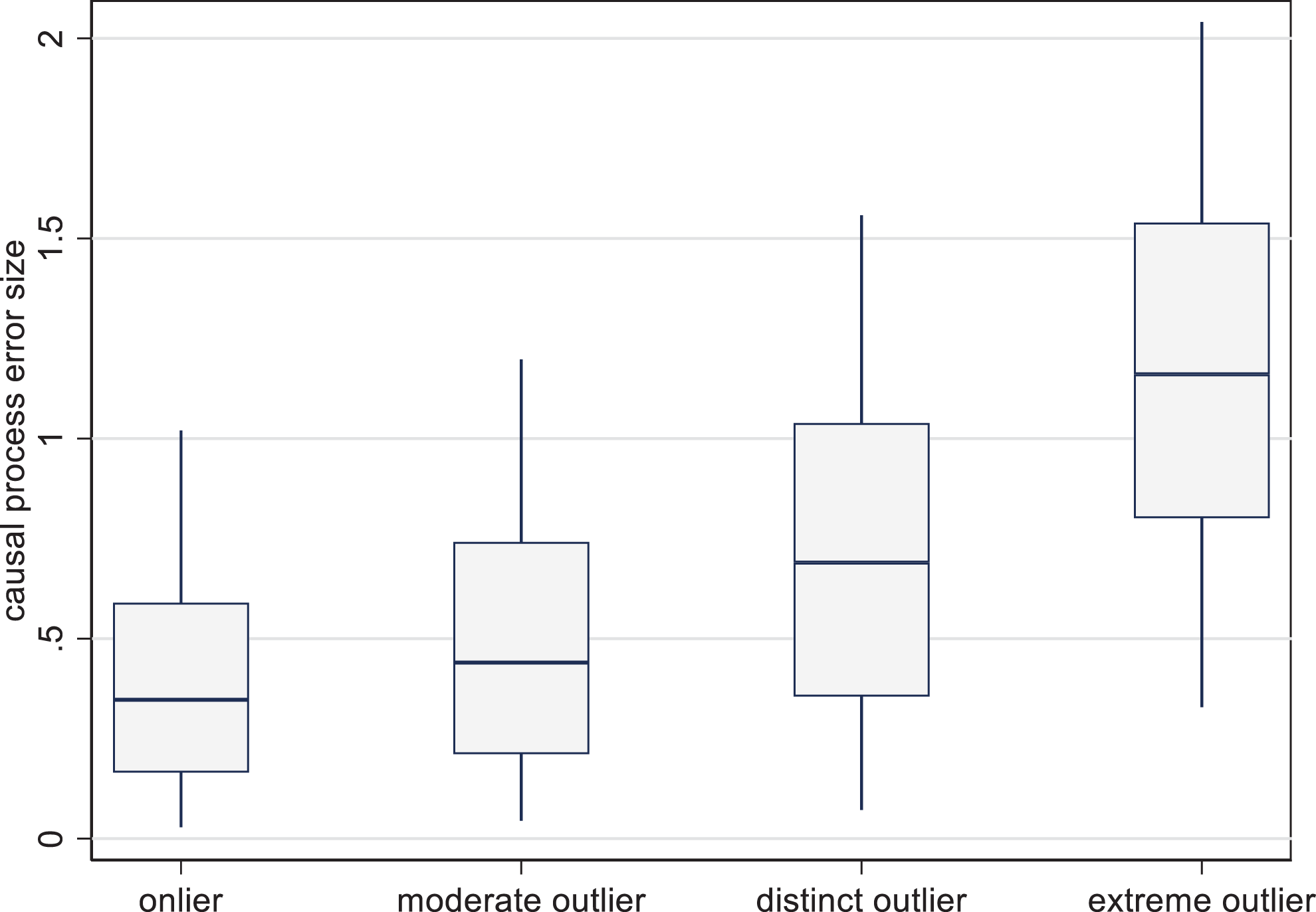
Simulated absolute causal process errors by outlier status.
Average of Absolute of Causal Process Errors.
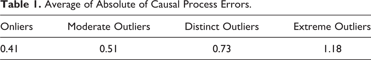
More important, however, is that onliers also have substantial average CPEs. To recall, the linear effects of X on Y in our model range from −1.5 to +1.5, so if we seek a case study that is representative in the effect size of the X–Y causal process, sizable distortions are possible even for onliers, given that their CPEs are also fairly widely dispersed, with 5 percent of onlier cases having CPEs above 1. Onliers are not necessarily representative. In our education-growth model, we might well end up choosing an onlier case with an unusually large or small effect of education on growth.
Conditions for False Negatives
We have so far worried about positive and negative causal errors. What if our concern is not unrepresentative causal effects in general, but only negative biases: substantially diluted, absent, or even reversed causal effects, that is, false negatives? The typical purpose of case studies is, after all, not the estimation of effect sizes but rather the detection of theoretically relevant causal mechanisms or pathways. If this is our aim, we should be more concerned about attenuated causal processes producing small effects than about unusually strong ones.
Attenuated effects occur in cases where CPEs reduce the size of the typical causal effect. This is more likely for cases that show a weaker effect on Y than the model predicts, which we call attenuating outliers. In these cases, at least some of their location below the regression surface will on average, though not always, be explained with CPEs. As we now focus on the direction of bias and not its absolute size, Figure 2 simply shows average CPEs. They are generated under the same case selection rules as in Figure 1, except that we only include cases with a negative residual, that is, where the Y is smaller than predicted. As expected, attenuating CPEs on average become larger the more negative the total residual is.
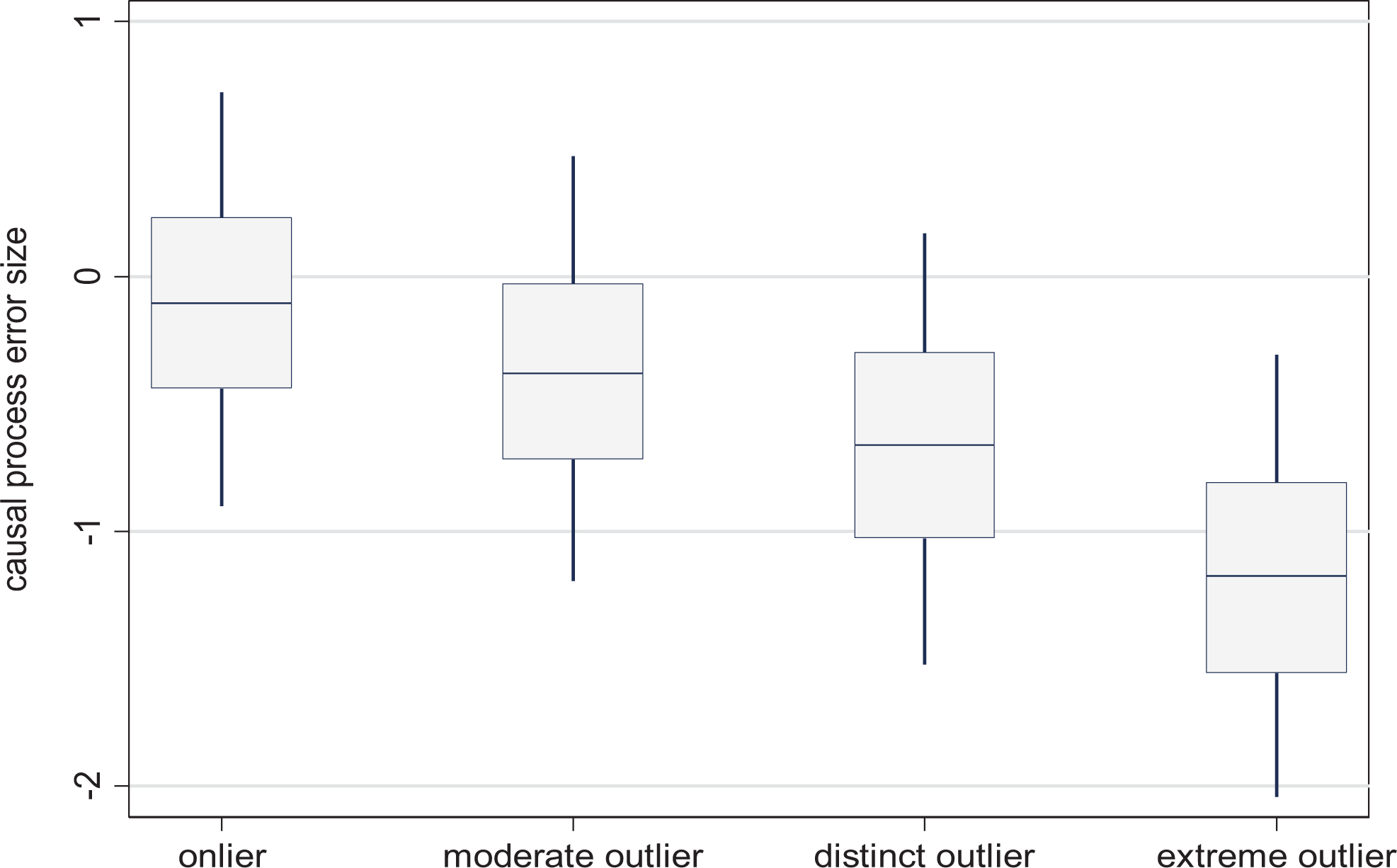
Simulated causal process errors by attenuating outlier status.
Unsurprisingly, for onliers with small negative residuals between zero and half of a standard deviation, there is little systematic bias in the CPEs, whose average, despite considerable dispersion, is −0.12. The systematic bias becomes much larger for stronger outliers and converges on the average of the absolute of CPEs for extreme outliers from Figure 1, as attenuating CPEs constitute virtually all of the CPEs in these cases.
How frequent are cases in which CPEs substantially reduce causal effects? The bottom three rows of Table 2 show the shares of cases in our four case categories that have CPEs below −0.71 (the CPEs’ standard deviation), −1, and −1.5. With a CPE of −0.71, even a case with an extreme X value of 3, that is, with the highest possible “leverage,” will lose almost half of the causal effect that it would typically have relative to the population mean. With a CPE of −1, it would lose two-thirds of its causal effect, and with −1.5, the causal effect would disappear, making it difficult if not impossible to detect the mechanism(s) underpinning it.
Average Incidence of Negative Causal Process Errors (CPEs) among Attenuating Outlier Cases.
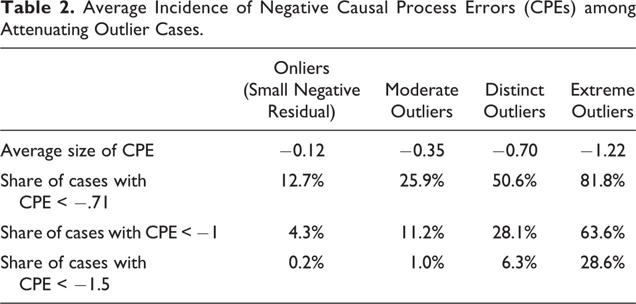
Under our assumptions, 12.7 percent of “high leverage” onlier cases would lose almost half or more of their causal effect due to CPEs, 4.3 percent would lose at least two-thirds, and 0.2 percent would lose their causal effects entirely and typically experience a reverse effect.
While we saw above that choosing onliers does not protect much against CPEs per se, compared to attenuating outliers they provide some insurance against large CPEs that substantially reduce or eliminate the X–Y causal effect. In our example, few onliers are at risk of complete attenuation of causal effects. We need to consider, however, that this results from a statistical model with a quite high R 2, which we moreover assume to be unbiased and subject to no measurement errors.
If we flatten the slope of the data generation process to
There are further reasons to believe that false negatives could be more frequent in research practice than in the above “clean” example: In smaller samples, there will often be no convenient onlier cases available that offers maximum leverage, creating a trade-off between onlier status and leverage. Model misspecification and mismeasurement further increase the risk of false negatives, as we might pick apparent onliers that are not onliers under a better model. We have also assumed the same standard deviation of CPEs for all values of X, while in practice, errors could be larger for onliers with more extreme values of X, which under simple regression models offer the highest leverage (Seawright 2016a).
In sum, the onlier rule provides reasonable but weak guidance in identifying typical cases and does not guard against false negatives if our LNA model is weak. Substantially, one can think of many reasons for why a causal process might not work or even produce the opposite of the expected outcome in specific cases. In the Collier and Hoeffler model, for example, primary commodity exports might in fact reduce the risk of conflict in a case where revenues are judiciously used for patronage and cooptation, a mechanism producing a pacifying effect. At the same time, other factors picked up by the background error, for example, militarization of society or high levels of organized crime, might in turn push the country toward a higher probability of war and hence back onto the regression surface, making it an onlier that is in fact not representative of general causal processes.
Our choice to make the CPE on average as large as the background error is arbitrary. This article’s basic arguments cover all ranges of CPEs, however: If we assume a smaller causal error, we are closer to a world of perfect causal homogeneity, which, as we have seen, offers no justification at all for onlier choices. For larger CPEs than assumed here, the onlier choice remains justified, but any observation—including onliers—will tend to be less representative, making generalization universally difficult. 4 This is equivalent to what happens when a model’s general explanatory fit is lowered as in the above example.
There is no obvious method for identifying the relative importance of CPEs relative to background errors in a model’s error structure. A researcher can only speculate how sensitive a hypothesized causal mechanism could be to idiosyncratic context factors and stochastic noise that we cannot model. More complex, higher level mechanisms might be more susceptible to be affected by context conditions: Macro-level processes like those linking education to growth or natural resources to conflict are more likely to be on the heterogeneous side. Qualitative cross-case comparisons might help researchers acquire a better, though not conclusive, sense of a mechanism’s dependence on idiosyncratic context.
While CPEs can always modulate case-level effect sizes, we have seen that under some conditions, the choice of onlier case studies makes it more likely that we will at least detect the presence and the mechanisms of a systematic causal process—even if the observed effect size is unlikely to be representative. But are onlier cases really the best choice if our objective is the detection and exploration of causal processes? For this, we should look for cases where the causal process is likely to be the most pronounced, hence most visible. Leverage is an obvious criterion for this, but onlier status is not. We will instead show that if we deliberately select outlier cases where the CPE is likely to strengthen the causal process of interest, false negatives are less likely than if we choose onliers.
Above we have looked at attenuating outliers where CPEs are likely to reduce the force of the causal process at hand. The flipside of this finding is that if we choose reinforcing outliers, their CPEs on average are likely to strengthen the causal process at hand. Ceteris paribus, a stronger reinforcing CPE should make process tracing easier due to the larger effect size.
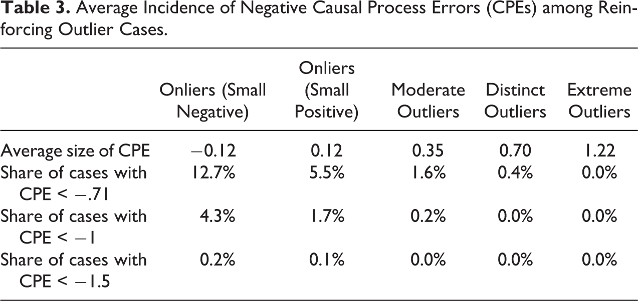
Table 3 shows the incidence of substantial attenuating CPEs for different types of outliers (see Online Appendix Section 2, Figure A.11, which can be found at http://smr.sagepub.com/supplemental/, for the corresponding figure). The results are clear: Even choosing only moderate reinforcing outliers strongly reduces the risks of CPEs that substantially weaken a causal process. Larger attenuating CPEs become unlikely if we choose reinforcing outlier cases. If the aim is to avoid the risk of false negatives, it pays to choose reinforcing outliers. In the education-growth example, this would mean choosing a country with somewhat higher than expected growth, thereby making it more likely that the education effect contributing to this growth is present and visible (if, on average, somewhat stronger than in the general case population).
Average Incidence of Negative Causal Process Errors (CPEs) among Reinforcing Outlier Cases.
Lieberman discusses the assessment we need to make when a nested case study does not bear out a hypothesis (Lieberman 2005:448): Is it just an idiosyncratic case subject to specific circumstances or measurement error? Or is something wrong with the hypothesis and perhaps the LNA used to choose the case? Any such discretionary judgment call will be open to potential criticism. That said, idiosyncrasies that suppress causal processes are less likely for reinforcing outliers: If we do not find a hypothesized process there, it is unlikely to exist elsewhere. Reinforcing outliers are also less vulnerable to measurement errors that can undermine the detection of a causal process: If Y is overestimated, the case will just be less of a reinforcing outlier unless the error was very large. If X was overestimated, the case just becomes a stronger outlier (with a potentially stronger causal effect). The same is true, conversely, about underestimated Ys and Xs. A mismeasured onlier case, by contrast, is more likely to actually be an attenuating outlier. 5
Conditions for False Positives
Choosing reinforcing outliers makes case-specific effect sizes likely to be somewhat larger than typical. But as noted above, the purpose of case studies is seldom to make point estimates of effect sizes—and in any case, the average absolute of CPEs in onliers barely differs between onliers and moderate outliers (Table 1). If anything, a somewhat larger effect is more likely to be visible and traceable, which is what we typically care about in small-n work (Seawright 2016b).
In our definition, the CPE captures case-specific factors that can boost or reduce a causal effect. If these are substantive rather than just stochastic, could a reinforcing outlier lead to false generalizations about the nature of the causal process at hand—a false positive? How important this problem is in research practice depends on whether we investigate a case with preexisting hypotheses about the X–Y causal mechanism or whether we try to identify the mechanism (or mechanisms) inductively through the case. In the latter context, the recommendation to choose reinforcing outliers needs to be qualified: 6 If proceeding inductively, we might mistake unsystematic elements of the CPE for a systematic, general causal process (Collier and Mahoney 1996). This can be the case for both onliers and reinforcing outliers, as both are subject to CPEs.
CPEs with a positive (observable) impact on the outcome are more likely for reinforcing outliers, however, just like attenuating CPEs are more likely for attenuating outliers in Table 2. Processes that create reinforcing CPEs are the ones we would be more likely to wrongly incorporate in our generalizing conclusions about the causal mechanisms at hand. In the case of natural resources and conflict, we might, for example, find that reliance on commodity rents allowed a country’s leadership to disengage from its social constituencies, in turn increasing the likelihood of conflict—but fail to realize that this process was case-specific. We might still be able to identify causal channels linking rents and conflict that are more general, but the risk of identifying idiosyncratic causal channels is higher for reinforcing outliers. We should at a minimum proceed with caution in assessing whether what we have found might “travel” to other cases.
Inductive research on causal mechanisms about a given X–Y link hence faces a trade-off between the risks of false positives (if reinforcing outliers are chosen) and false negatives (if onliers are chosen). This trade-off should be explicitly evaluated on case-by-case basis. If a project will lead to follow-up case study or LNA tests of the external validity of new findings on causal mechanisms, a more exploratory choice of reinforcing outliers might be advisable, as otherwise an important process might be missed. If, by contrast, there are resources for only one case study, an onlier case choice is a conservative strategy that somewhat reduces the risk of false positives. This is especially so if an X–Y link has a high ex ante likelihood of being affected by idiosyncratic processes.
The situation is different for case studies that test preexisting hypotheses about a causal process: Unless these hypotheses have been generated by the case at hand, any case will be a reasonable test of their generalizability. It is unlikely that a preexisting hypothesis perchance only applies in one case, that is, that we find a false positive. 7 It is at the very least likely to also apply in some other cases—although we cannot conclude that it is universal or estimate its frequency, which is the domain of large-n research.
Under these circumstances of hypothesis testing, it is most appropriate to choose reinforcing outliers as argued above, as in such cases, general causal processes are more likely to be strong and visible. Reinforcing outliers are also useful for falsification, as they effectively constitute “most likely” cases—if a hypothesis does not apply there, it is less likely to apply elsewhere.
Onliers and attenuating outliers, by contrast, run a substantial risk of yielding a false negative in research designs that investigate existing hypotheses, for reasons identified above. If a hypothesized causal process is absent or substantially weak in such cases, we will not know whether this is due to the case’s idiosyncrasies or because the causal process hypothesis is wrong. 8
In practice, even deductive research designs can create new causal process hypotheses, or new nuances to existing hypotheses, in the process of case research. But if we identify such new dimensions, we should be careful about generalizing from them, as they might constitute part of a reinforcing CPE. As with general inductive research, such theoretical adjustments should ideally be subjected to further tests on other cases or, if possible, a modified LNA. In the context of primary resources and civil war, for example, we might investigate a resource exporting country in which high levels of corruption in the distribution of rents have contributed to the greed and disaffection leading to war. This could lead us to add an interaction between a corruption measure and resource exports in the LNA model.
If what we find appears intuitively plausible for a larger share of cases, the question whether the case at hand was an onlier or not should be secondary in deciding about LNA model revisions. If the new specification provides no leverage in the revised LNA, this suggests that the additional nuances we have detected were case-specific. If a revised causal process hypothesis cannot be tested in the LNA, the best way of assessing its generalizability is to study at least one more case for which it then becomes an ex ante hypothesis. In this case, as per the above discussion, a reinforcing outlier should be chosen.
The above discussion highlights the critical importance of a clear research protocol, that is, of establishing and documenting at which stage hypotheses are generated and when they are tested. This is critical for deciding which type of case to choose in nested research designs. Nonexperimental political science still does not pay much attention to documenting research designs ex ante (Humphreys, de la Sierra, and van der Windt 2013).
The above guidelines are quite different from standard rules of case choice in the mixed methods literature. The one author who suggests the deliberate choice of outliers is Seawright. He rightly, if fairly briefly, points out the value of deviant cases for investigating causal pathways between known X’s and Y’s, given that intervening causal processes in such cases can be stronger and more visible (Seawright 2016a, 2016b:86). In this article, we make the implicit distinction between CPEs and background errors underlying this recommendation explicit and, reinforcing the utility of outliers, demonstrate how “typical” cases can still be unrepresentative. We add the critical distinction between reinforcing and attenuating outliers (rather than focusing on deviant cases in general) but also explain how the risk of false positives demands different case choices depending on whether we investigate causal processes deductively or inductively.
For the sake of exposition, the randomly generated data in the above discussion were based on a simple bivariate regression model. The basic logic of our arguments holds under wide range of assumptions and model variations; see Online Appendix Section 3, which can be found at http://smr.sagepub.com/supplemental/, for a discussion of multivariate and discrete outcome models, models with nonlinear effects and for case studies that investigate several independent variables at once.
Causal Process Errors and Other Case Selection Objectives
Our interpretation of causal heterogeneity also has implications for other purposes of case selection beyond the investigation of mechanisms. First, if we allow for the possibility of CPEs, using case studies for estimating general effect sizes for larger populations—a relatively unusual approach yet one advocated in recent literature (Herron and Quinn 2016)—is a highly unreliable enterprise.
When it comes to diagnostic case studies for identifying measurement error on the outcome variable, unobserved (nonconfounder) variables, and systematic causal heterogeneity, existing prescriptions to use deviant cases (Seawright 2016a) continue to make sense. Yet we need to allow for the possibility that deviance is just an outcome of unsystematic causal heterogeneity, including particularly weak or powerful versions of a general, already known causal mechanism. A single case study is not necessarily dispositive in identifying any of the above factors.
To the extent that case studies are used to test for endogeneity in the shape of reverse causality, we can use analogous rules as for the detection of conventional causal mechanisms: A reverse mechanism linking the outcome variable to the (assumed) causal variable will again on average be more visible for reinforcing outliers. But as the X and Y axes are flipped in the case of reverse causality, the cases where the mechanisms underlying reverse causality are likely to be stronger are in fact attenuating outliers from the perspective of the X–Y model. This requires us to simply reverse the above selection rules. Intuitively, if we wanted to assess whether economic growth causes education rather than the other way around, we would look at cases where growth is combined with especially high education, making it more likely that the effect of growth on education is visible.
Finally, if the objective is to detect omitted variables that act as confounders (i.e., are related to both the independent and dependent variable in our model), the choice of outliers is of no particular use. Confounders are not systematically stronger for outliers: As confounders affect both X and Y, a strong confounder would just affect both simultaneously rather than systematically pushing cases off the regression surface. Researchers should instead follow Seawright (2016a) in picking “high leverage” cases with values of the independent variable with the strongest predicted impact. Again, we need to be aware of the uncertainty involved in any case-specific inferences: Any confounder process itself could be subject to CPE and can be idiosyncratically strong or weak.
A Defense of Paired Case Comparisons
So far, our discussion has looked at the investigation of individual cases, similar to the “pathway case” approach recommended by Gerring (2007b). How helpful is it to investigate more than one case for the process tracing of mechanisms, as recommended by Lieberman (2005:441)? What is the impact on the reliability of our findings under the CPE framework? It turns out that this framework provides a new and strong justification for traditional approaches to paired comparison (Slater and Ziblatt 2013; Tarrow 2010), especially “method of difference”-type setups with contrasting outcomes across cases. This is significant because the value added of such comparisons has been in doubt ever since Lieberson’s (1991) trenchant criticism of the use of Mill’s methods of comparison in social science.
To be sure, if we investigate two cases, causal heterogeneity means that the probability of finding at least one false negative increases significantly compared to a single case study (see Table 4 compared to Tables 2 and 3; for a graphical representation of attenuating CPEs in paired comparisons, see Figure A.12 in Online Appendix Section 2, which can be found at http://smr.sagepub.com/supplemental/). The risk that in one of two countries under study education has an unusual effect on growth is higher than in a single case study.
Average Incidence of at Least One Negative Causal Process Error (CPE) among Two Outlier Cases.
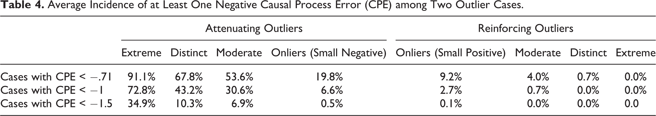
If we are testing preexisting hypotheses, a mixed finding with one false negative might lead us to conclude that the process at hand is likely to apply in some cases but not others and that we are dealing with an issue of group-level causal heterogeneity—while in fact, net of case-specific, idiosyncratic errors, the causal process identified in the other case is general. If we arrive at mixed findings inductively, the (wrong) suspicion that what we have found is idiosyncratic and not generalizable will be even stronger.
The above might seem dispiriting for comparative scholars. But it applies only if the two case studies are dealt with as separate investigations. In this context, we expect their outcome scores to be implicitly compared to the population mean, net of statistical controls. In a properly executed paired comparison, however, we compare outcomes between the cases. If—as Lieberman suggests—cases are chosen at opposite ends of the leverage spectrum, the contrast between their outcomes will be larger.
In this context, we should look at the comparison as one integrated research design. We need to consider the probability that we will find the same or similar causal processes (or absence thereof) in two cases if they have been chosen with contrasting leverage on the independent variable of interest. Identifying cases this way extends Seawright’s (2016b) recommendation to choose extreme values on the independent variable from the choice of single cases to the choice of case pairs.
We consider pairs of cases chosen at opposite ends of the X spectrum in our above bivariate simulation with random CPEs and background errors. We investigate the combined CPEs from different, randomly drawn case pairings with different levels of outlier status, including both attenuating and reinforcing outliers, similar to Figure 1 and Table 1.
Table 5 indicates that the combined attenuating effect of two cases’ CPEs very rarely is strong enough to obliterate the whole difference in causal effects across the two cases. The linear effects of X on Y in our model range from −1.5 at one extreme to +1.5 at the other. This means that the combined CPEs would have to “push” the two cases closer together by three points on the Y scale for the causal processes to evince no difference in both, which happens very rarely under the chosen data generation process (see Figure A.13 in Online Appendix Section 2, which can be found at http://smr.sagepub.com/supplemental/, for a graphical representation of combined CPEs).
Incidence of Combined Causal Process Errors (CPEs) of Paired Observations (All Types of Outliers).
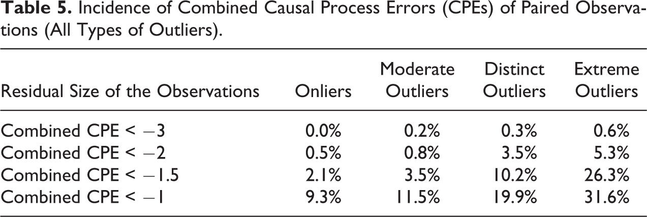
The risk of a false negative becomes larger if we choose case pairs in which the individual cases have larger, randomly chosen residuals. It grows also if we choose case pairs whose X scores are closer to each other. A combined CPE equivalent to two points on the Y scale, which implies a reduction of two-thirds of the difference in X’s effect between two extreme cases, happens in 3.5 percent of case pairs consisting of distinct outliers. In a data generation process with a lower X gradient of
Choosing onliers is better than random choice of outliers. But what about choosing outliers strategically? Similar to our strategy of choosing reinforcing outliers in a single case study, we now choose cases whose outcomes lie further apart than the model suggests, which typically (though not always) are cases with residuals of opposite signs. In combining such cases, we are even less likely to have combined CPEs that attenuate the contrast between the two cases. Table 6 shows that the procedure does indeed result in even fewer false negatives, particularly if we choose cases further away from the regression surface, including moderate outliers, which are barely more likely to be atypical than onliers (see Online Appendix Section 2, Figure A.14, which can be found at http://smr.sagepub.com/supplemental/, for a graphical representation). This selection strategy of contrasting residuals is particularly advisable if our statistical models are weak. It means that CPEs across cases can do less damage: One case or even both might be unusual, but the size of the (deliberately chosen) contrast across cases tends to more than compensate for this.
Incidence of Combined Causal Process Errors (CPEs) of Paired Observations with Contrasting Residuals.
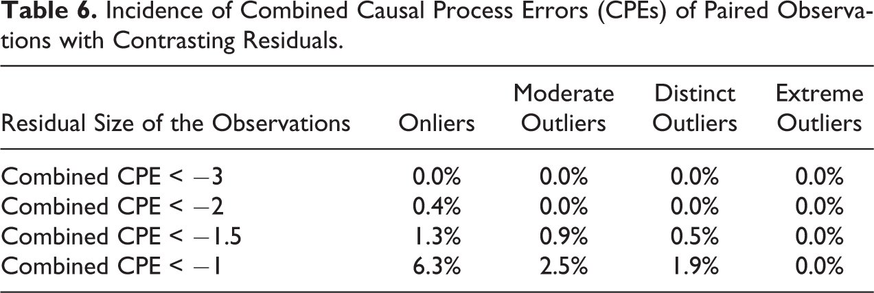
To return to the education-growth example: If we compare a case with low educational attainment and particularly low growth outcomes with a case with high educational attainment and particularly high growth outcomes, it is unlikely that the difference in education levels has not contributed in at least some way to the difference in growth across the two cases through observable mechanisms.
Qualitative methods literature argues that investigating a contrasting case helps understand one’s core case better (Tarrow 2010:17) and that comparisons should capture the full variation of outcomes (Slater and Ziblatt 2013). Our framework provides a formal justification for these intuitions.
Different from single-case nested research, in the case of comparisons, the same essential logic applies to deductive and inductive process tracing. The main difference is that the inferential payoff from comparisons is larger for inductive research: Not only does the choice of contrasting outliers lower the risk of attenuated effects and make it more likely that contrasting causal processes will be visible. To the extent that the two cases at hand show variations of the same process, this process is much more likely to be generalizable. This means that comparisons are particularly advisable for inductive research on causal processes.
The analysis of paired case studies also helps with identifying cases for exploratory research that serve to identify new independent variables which could be added to an LNA model (“deviant” cases in Gerring’s terminology and “model-building” case studies in Lieberman’s). Both Lieberman and Gerring counsel the deliberate choice of outliers to detect new causal processes. In case of a weak LNA, outlier status does not tell us much per se (Rohlfing 2008). If we however choose cases with contrasting outcomes on the dependent variable that also have contrasting residuals as outlined above, we are more likely to detect systematic factors that drive the two apart. Such a research design could be potentially strengthened if the cases are matched on other measurable criteria (Nielsen 2016).
The only qualification to the rule of choosing contrasting outliers obtains if cases with a low value of the X variable at hand simply reflect the absence of a cause, which can be the case especially with zero-bounded variables. If our objective is to establish whether a causal process is general, including a case in which the process can by definition not be present in our comparison is not useful. If our aim is to research the causal processes through which resource exports make civil war more likely, a case without resource exports will not allow us to process trace the link between resources and conflict. It will at best serve as broad contrast to another case with resource exports. In such circumstances, it is advisable to choose two reinforcing outliers with the causal factor (strongly) present.
Whether we can think of a causal factor as absent when it takes low values is easier to decide in a deductive research design based on a specific theory of how that factor brings about the outcome. It can be harder in inductive research designs without hypotheses about the causal mechanism. In case of doubt, one should err on the side of caution by choosing two reinforcing outliers. Investigating two cases with similar values on the independent variable instead of just one does increases the risk of at least one false negative, but the baseline that these cases are contrasted with is the complete absence of the independent variable. If we choose two cases with an X value of 3 in our model, even a large attenuating CPE of −1.5 would diminish the impact of the independent variable only by half. The choice of reinforcing outliers further reduces the risk of false negatives (see Table 3). While we are not able to leverage cross-case contrasts in a comparison of two reinforcing cases, if a process is indeed found in both cases, we can be more confident in its generality. This point is less important for deductive research designs—where a single case study with a positive finding already carries considerable weight—but can be critical for replicating the results from inductive investigations on a first case. 9
The above discussion has important implications for single case studies too: If a causal variable is theorized as simply absent at its lower boundary, with no specific expectation of observable mechanisms, the visibility of effects at the upper range of the variable in a single case is potentially larger. This is because, as above, we are not comparing our observations to the population mean as in our above discussion of causal variables that we expect to have contrasting effects at both ends of their value range. We instead implicitly compare a mechanism at the high end of the causal variable’s range with its (theoretical) absence at the opposite end of the range. How much of an advantage this simpler setup constitutes will in practice depend on the strength of a causal process and its error structure. In any case, the same rules for choosing reinforcing outliers apply as for other single case studies; see Online Appendix Section 4, which can be found at http://smr.sagepub.com/supplemental/, for additional simulations of causal effects and CPEs that converge toward zero at one end of the causal variable’s range.
While it might appear counterintuitive to large-n scholars, the addition of a second, well-chosen case to a small-n research design can make empirical inferences significantly more robust. Our discussion confirms Lieberman’s advice to focus on at least two cases, providing a formal justification for paired comparisons that has so far been lacking in the small-n methods literature. Critically, our arguments apply for paired comparisons in general, not only ones that are nested in an LNA.
Discussion: Implications for Research Practice
Imagine we build a statistical model explaining voter attitudes based on survey data. The model is then used to identify one individual respondent who is chosen for a case study on how and why wealth impacts citizens’ political self-identification because (a) she is very wealthy and (b) her score on the outcome variable of left-right placement produces a small residual in the statistical model. Further imagine that with superhuman finesse, we are able to explain the factors that shaped her political position through a detailed biographical investigation. Having accounted for all other systematic and case-specific context factors in this case, we then isolate the impact that wealth has had and the mechanisms involved. We finally conclude that thanks to the small residual, the mechanisms identified are likely to capture how wealth influences political positions in the voting population in general.
This story is absurdly heroic, yet it summarizes what nested research designs often ask us to do. We should be all the more skeptical about standard case identification procedures in such research designs if they involve more complex and more variegated units of analysis such as social groups, organizations, or states. 10 As long as we believe that we live in a stochastic world, any generalization from case studies—whether embedded in large-n research designs or not—needs to be provisional and undertaken with the utmost caution. This article provides a new conceptual framework for understanding the roots of uncertainty in such generalizations.
Mario Small has argued that we can never reach statistical representativeness in small-n samples and should not aim for it. Deliberately picking “typical” neighborhoods or households for in-depth study is misguided (Small 2009). Instead, case should be picked on theoretical grounds and aim at “theoretical generalization,” that is, demonstrating patterns that are of broader theoretical significance, without making any claims about empirical regularities. He makes this case in the context of disciplines like social work and sociology, where “small-n” usually means at least four and typically dozens of cases, that is, more than in most political science nested research designs (Creswell and Clark 2010; Small 2011).
This article is not quite as pessimistic as Small. We cannot use small-n samples to generalize reliably about effect sizes and the frequency of specific causal patterns in a wider class of cases. Yet, under some conditions, we can make plausible claims that causal mechanisms identified in small-n research also apply in other instances. This article has identified these conditions and developed guidelines to reduce the risk of false generalizations from small-n work nested in large-n studies.
In its analysis of nested case choice, this article has shown that the size of causal effects is likely to fluctuate in both onlier and outlier cases. But estimates of effect size are not the primary concern of most case study research. Instead, in many instances, we want to establish whether a causal process exists and investigate its nature. Table 7 gives an overview of the rules for doing so that emerge from our discussion. Critically, our case selection strategy should take into account our state of knowledge: If we have existing hypotheses about the process(es) at hand, in a single case study, it is most advisable to investigate reinforcing outliers, as this makes the presence, strength, and visibility of a given causal process more likely, facilitating process tracing (column 1 in Table 7). Reinforcing outliers have a smaller risk of false negatives, while false positives in hypothesis-testing research are unlikely.
Case Choice Rules for Nested Analysis of Causal Mechanisms.
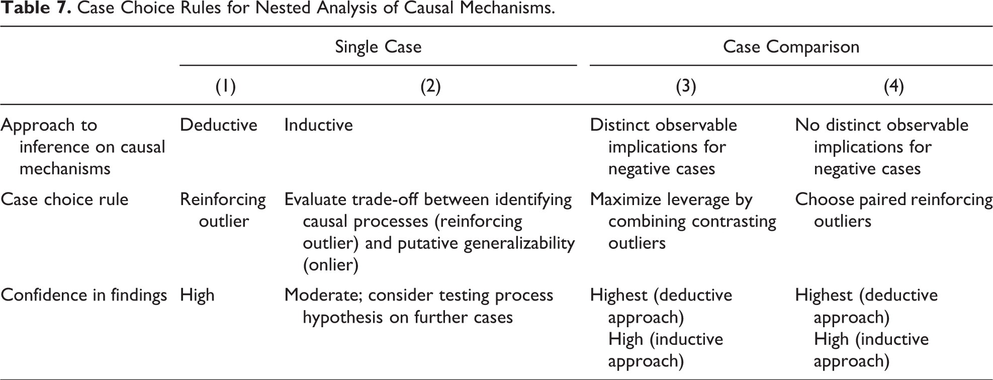
If our objective is to inductively identify causal mechanisms linking a given independent variable with an outcome (column 2), reinforcing outliers make it more likely that general causal patterns are more visible. If we want to generalize about these processes, however, reinforcing outliers also increase the chance that the identified causal processes, or aspects thereof, are idiosyncratic. In some cases, it will be theoretically or intuitively obvious whether a specific process is likely to apply to a wider population, but in others, it will not be. Choosing onlier cases for the inductive identification of causal processes makes false positives less likely but increases the risk of false negatives. As onliers can also be subject to causal process errors, inductive generalization about causal mechanisms on the basis of individual case studies is generally tenuous. Such generalizing inferences can be every bit as problematic as using case studies to generalize about causal effects, a problem that is more clearly recognized in the mixed methods literature (Gerring 2004:348; Lieberman 2005:441). Inductive research about causal processes hence faces a trade-off between false negatives and false positives. How this is resolved will depend on the purpose and context of the project at hand, but the trade-off should in any case be made explicit.
We have seen that increasing the number of cases under study can work as partial corrective to case-specific errors. This is especially the case if we can pair cases in a joint research design that maximizes the contrast in the causal variable at hand, thereby minimizing the risk of false negatives. Ceteris paribus, this procedure is considerably more robust than single “pathway” case studies. It only works, however, if there are distinct observable implications for contrasting values on the independent variable (column 3).
If that is not the case—if one end of the contrast only implies absence of a causal process—it is more advisable to choose two reinforcing outlier cases with a strong expected impact on Y (column 4) as replication cases. If a causal mechanism is visible in both cases, it is quite likely to also recur in the larger universe the cases are sampled from. This is especially the case for deductive tests of mechanisms, but it is also likely even if the mechanism is identified inductively. 11 That said, if we truly want to generalize about frequency and strength of causal mechanisms, we have to do this through LNA methods (Barnes and Weller 2014; Imai et al. 2011). In practice, this will often not be possible due to lack of data, incommensurability of measures across cases and the statistical difficulty of separating a mechanism’s immediate impact from the related independent variable’s residual impact (Imai et al. 2011).
This article has also used its framework to refine case selection rules for other research purposes such as identifying new causal variables, confounders, measurement error, and reverse causality. It mostly supports preexisting selection approaches in these cases, but with a note of caution about generalizability. It provides a new rule for selecting attenuating outliers for identifying mechanisms that underlie potential reverse causality.
If this article’s arguments seem complex, then this is because the use of large-n methods to identify appropriate case studies in a statistical context necessarily involves complex assumptions that have not been sufficiently analyzed to date. The argument over causal process errors is difficult to avoid if we want to stick with formal techniques of small-n case choice. If this article’s more differentiated recommendations for choosing cases appear complex and contingent, then the broader conclusion that we need to be generally more modest about our mixed methods ambitions, and about generalization from case studies more broadly, remains all the more valid.
Case studies continue to be very important in their own right for producing internally valid accounts of what happens in individual cases, and they arguably remain the primary tool of hypothesis generation for large-n studies. But when we want to generalize from them, we need to apply more differentiated rules than simply choosing “on the line,” be more attentive to substantive context as well as chance, and more tentative about the external validity of our findings.
On the most general level, researchers using statistical methods need to take these methods’ assumptions about how causality works seriously and, to be consistent, carry them into their case studies. This means that case-level causal effects are, ex ante, unknowable and mechanisms, when detected, potentially unrepresentative. If we want to reliably generalize with small-n methods, we need to put more focus on replication. One unexpected ray of light in this context is that small-n comparisons—much less discussed in the methods literature of the last 20 years than single case study selection methods—improve the chances of externally valid findings substantially in a stochastic world. They deserve further study by methodologists, especially those working in a mixed methods paradigm.
Supplemental Material
Supplemental Material, sj-pdf-1-smr-10.1177_0049124120986206 - Taking Causal Heterogeneity Seriously: Implications for Case Choice and Case Study-Based Generalizations
Supplemental Material, sj-pdf-1-smr-10.1177_0049124120986206 for Taking Causal Heterogeneity Seriously: Implications for Case Choice and Case Study-Based Generalizations by Steffen Hertog in Sociological Methods & Research
Footnotes
Declaration of Conflicting Interests
The author(s) declared no potential conflicts of interest with respect to the research, authorship, and/or publication of this article.
Funding
The author(s) received no financial support for the research, authorship, and/or publication of this article.
Supplemental Material
Supplemental material for this article is available online.
Notes
References
Supplementary Material
Please find the following supplemental material available below.
For Open Access articles published under a Creative Commons License, all supplemental material carries the same license as the article it is associated with.
For non-Open Access articles published, all supplemental material carries a non-exclusive license, and permission requests for re-use of supplemental material or any part of supplemental material shall be sent directly to the copyright owner as specified in the copyright notice associated with the article.