The Integration of Bayesian Regression Analysis and Bayesian Process Tracing in Mixed-Methods Research

Abstract

In this article, we develop a mixed-methods design that combines Bayesian regression with Bayesian process tracing. A fully Bayesian multimethod design allows one to include empirical knowledge at each stage of the analysis and to coherently transfer information from the quantitative to the qualitative analysis, and vice versa. We present a complete mixed-methods workflow explaining how this is accomplished and how to integrate both methods. It is demonstrated how to use the posterior highest density interval and the Bayes factor from the regression analysis to update the prior level of confidence about what mechanisms possibly connect the cause to the outcome. It is further shown how to choose cases for the qualitative analysis through posterior predictive sampling. We illustrate this approach with an empirical analysis of colonial development and compare it with alternative designs, including nested analysis and the Bayesian integration of qualitative and quantitative methods.

Introduction

In the development of mixed-methods designs in political science, nested analysis marks an important contribution by overcoming the dichotomy between qualitative, small-n and quantitative, large-n studies that, prior to the early 2000s, was characteristic of political science research (Lieberman, 2005). The mixed-methods design covers the familiar $\mathit{X}\mathbf{\to }\mathit{M}\mathbf{\to }\mathit{Y}$ scheme (e.g., Gerring, 2008) by estimating the effect of the main variable of theoretical interest, $\mathit{X}$ , on the outcome, $\mathit{Y}$ , and collecting qualitative evidence on the mechanism $\mathit{M}$ that explains the presence of an effect. ¹ The close integration of the two methods is achieved by building the case studies on the estimates of a frequentist regression. ² The development of nested analysis was the starting point for follow-up research focusing on elements such as concept formation (Ahram, 2013), and case selection strategies that depart from the original recommendations (Seawright, 2016a; Weller and Barnes, 2016; Hertog, 2023). This type of mixed-methods design has its origins in political science, but is also relevant for sociology that has a longstanding and rich tradition of mixed-methods research (MMR) (Small, 2011). Empirical applications demonstrate that this integrated design can be used to answer substantively motivated sociological research questions (Go, 2020; Somma and Bargsted, 2018).

We contribute to the advancement of multimethod research by developing a Bayesian mixed-methods design that combines a Bayesian regression analysis with Bayesian process tracing. Our motivation is twofold. First, nested analysis is presented as “folk Bayesianism” by “introducing investigator knowledge to the world” (Lieberman, 2005). From a Bayesian perspective, its original frequentist formulation stops midway because one is not able to formally incorporate existing knowledge and transfer information from one design stage to the next. We show how Bayesianism allows one to include empirical knowledge at each stage of the analysis and to pass forward information from one stage to the next. We explain how Bayesian regression analysis can inform follow-up process tracing and how the qualitative insights gained can be linked back to the quantitative analysis. This allows one to turn “folk Bayesianism” into a formalized Bayesian framework that gives researchers the flexibility to combine regression analysis with formal, quantified process tracing, or informal process tracing that works with verbal classifiers such as “strongly in favor,” “moderately in favor,” and so on. Second, by following our proposed approach, researchers intending to perform Bayesian process tracing, which appears to become increasingly popular in empirical research, can seamlessly integrate it with a Bayesian regression.

The focus of the article is on the following four points. First, the Bayes factor for the regression estimate of $\mathit{X}$ can quantify the strength of evidence that the effect is negative as opposed to positive or null. We show how to use the Bayes factor, representing an element of testing in Bayesian regression (Kruschke and Liddell, 2018), by inferring how much it changes confidence that a mechanism is present. The updated level of confidence in a mechanism informs the decision about the amount of resources one should expend on collecting evidence on a specific mechanism. Second, we show how one can infer the range of the most probable effects of $\mathit{X}$ from the posterior highest density interval as an element of estimation (Kruschke and Liddell, 2018). Under certain assumptions, the location and width of the highest density interval allow one to derive expectations about the expected strength of the process tracing evidence. Third, we demonstrate the use of the posterior predictive distribution for the choice of cases, taking into account sampling uncertainty as well as uncertainty about the effect size. Fourth, we illustrate the integration of existing qualitative knowledge into the initial large-n analysis through the specification of prior distributions for regression parameters. What we do not illustrate in this article is a complete realization of a Bayesian mixed-methods design that includes a qualitative Bayesian analysis. Standalone Bayesian qualitative research, which has been discussed in much detail already (Abell, 2009; Fairfield and Charman, 2022; Zaks, 2017), is not part of our work because we focus on the unique elements of integrating the quantitative and qualitative parts in a multimethod design.

For the presentation of the Bayesian mixed-methods design, in the “Empirical Example: British Colonial Rule, State-Legal Capacity, and Development” section, we introduce an analysis of the development of former British colonies by Lange (2009) as the leading empirical example. We use this as a template for introducing the Bayesian workflow in “The Elements and Workflow of the Bayesian Design” section and illustrate the means by which Bayesian regression is integrated with process tracing in the “Illustration: British Rule and Colonial Development” section. In the Supplemental Appendix and“Illustration: British Rule and Colonial Development” section, we supplement the example with Monte Carlo simulations for a variety of parameter constellations. The “Comparison With Other Mixed-Methods Approaches” section clarifies the differences and commonalities of our Bayesian mixed-methods design with alternative mixed-method approaches. The final section concludes the article.

Empirical Example: British Colonial Rule, State-Legal Capacity, and Development

The leading empirical example is a study of the effects and mechanisms of the type of British rule on the socio-economic and political development of former British colonies (Lange, 2009). We introduce the theoretical argument to establish a basis for the following sections. Our primary aim is neither to make a contribution to this field of research nor to criticize it. Lange’s analysis is exemplary in following the standards set by Lieberman (2005). We discuss the design and the empirical strategy in the “Illustration: British Rule and Colonial Development” section.

On the macro level, the hypothesis is that more indirect British rule leads to worse socio-economic and political development than more direct British rule. ³ Direct rule is defined as the dismantling of existing institutions in the colony and the creation of new, bureaucratic-legal institutions run by colonial officials. Indirect rule follows a collaborative model that leaves the colony’s institutions intact in the periphery and complements them with British bureaucratic institutions in the center (Lange, 2009). In the following, we refer to the main independent variable $\mathit{X}$ as the ‘degree of indirect rule'.

The negative effect of more indirect rule works through a mechanism having multiple components. Figure 1 summarizes the mechanism presented by Lange (2009). ⁴ First, more indirect rule produces weaker legal-administrative institutions throughout the country; second, it undermines inclusiveness because of a lack of regular interactions between the colonial state and society; and third, it weakens infrastructural power because of the absence of colonial officials and legal-administrative institutions throughout the country. A weaker bureaucracy and infrastructure further reduce inclusiveness. All three elements together represent a weakened legal-administrative capacity, which is why we refer to the mechanism in Figure 1 as the “legal-administrative capacity mechanism” or simply the ‘capacity mechanism'. By the end of this process, development is worse than in a more directly ruled colony where all relationships are reversed.

Figure 1.

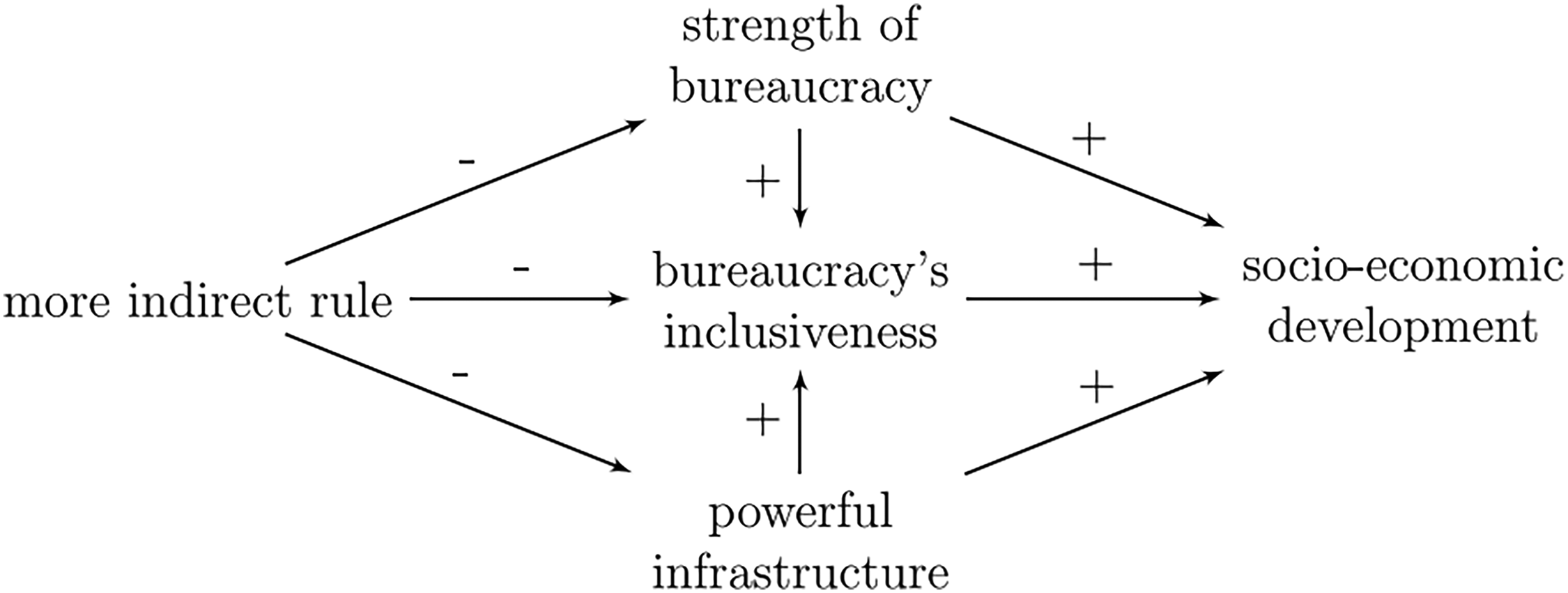
Theoretical model by Lange (2009).

For the purpose of presenting the Bayesian design, we introduce formal notations for the various elements of the theory and analysis (see for a summary of the formal notation Supplemental Appendix Section A). We generally refer to a parameter estimate in the quantitative analysis as $\mathit{\theta }$ and denote a negative parameter estimate as ${\mathit{\theta }}_{\mathit{N}\mathit{E}\mathit{G}}$ . We refer to the hypothesized or inferred negative effect of a variable $\mathit{X}$ as ${\mathit{X}}_{{\mathit{\theta }}_{\mathit{N}\mathit{E}\mathit{G}}}$ . The hypothesis of a negative effect is specified as $H_{{\theta }_{NEG}}$ . We represent the mechanism of focal interest associated with a negative effect with ${\mathit{M}}_{\mathit{N}\mathit{E}\mathit{G}}$ (or ‘negative mechanism') and the hypothesis that the negative mechanism is present as $H_{M_{NEG}}$ . ⁵

In a Bayesian analysis, we need a competing hypothesis because Bayesianism is inherently comparative. Based on colonialism research that was available when the analysis was done, one could have expected that more indirect rule would have a positive effect on development (see the “Illustration: British Rule and Colonial Development” section and Supplemental Appendix Section D.2). ${\mathit{\theta }}_{\mathit{P}\mathit{O}\mathit{S}}$ stands for a positive parameter estimate of more indirect rule; ${\mathit{X}}_{{\mathit{\theta }}_{\mathit{P}\mathit{O}\mathit{S}}}$ for the hypothesized or inferred positive effect of ‘degree of indirect rule'; ${\mathit{M}}_{\mathit{P}\mathit{O}\mathit{S}}$ for the associated mechanism; and $H_{{\theta }_{POS}}$ and $H_{M_{POS}}$ represent the hypotheses on the positive effect and mechanism, respectively.

Using this formalization, we can make the $\mathit{X}\mathbf{\to }\mathit{M}\mathbf{\to }\mathit{Y}$ scheme more specific. An independent variable does not cause a particular mechanism per se because the nature of the mechanism depends on the direction (or type) of the effect of $\mathit{X}$ on $\mathit{Y}$ . The index $d$ serves as a placeholder for the hypothesized or inferred direction of the effect and associated mechanism that is dependent on it: ${\mathit{X}}_{\mathit{d}}\mathbf{\to }{\mathit{M}}_{\mathit{d}}\mathbf{\to }\mathit{Y}$ . ⁶ This modified scheme allows us to simplify Lange’s argument to the causal chain ${\mathit{X}}_{{\mathit{\theta }}_{\mathit{N}\mathit{E}\mathit{G}}}\mathbf{\to }{\mathit{M}}_{\mathit{N}\mathit{E}\mathit{G}}\mathbf{\to }\mathit{Y}$ , as a negative effect of more indirect rule is expected to trigger the associated mechanism. The counterhypothesis of a positive effect of more indirect rule is ${\mathit{X}}_{{\mathit{\theta }}_{\mathit{P}\mathit{O}\mathit{S}}}\mathbf{\to }{\mathit{M}}_{\mathit{P}\mathit{O}\mathit{S}}\mathbf{\to }\mathit{Y}$ . The two hypotheses about a negative and a positive effect are complemented by the conventional null hypothesis $H_0$ stating a null effect, ${\mathit{\theta }}_{\mathbf{0}}$ , and the expectation that no systematic mechanism is present. We mainly focus our discussion on the comparison of a negative effect and mechanism with a positive effect and mechanism. All our arguments generalize to a comparison of a directional hypothesis with the null hypothesis. ⁷

The Elements and Workflow of the Bayesian Design

Mixed-methods research that combines a large-n and small-n method in this order has three interactive elements. We formulate these elements as questions that guide the discussion. First, what mechanism can one expect to be in place in process tracing based on the quantitative results? Second, how confident can one be that this mechanism is present and how many resources should we focus on collecting evidence for this mechanism and not others (on resources, Bennett, 2015)? $X_d\to M_d$ The two questions are aimed at determining what the placeholder $M_d$ should be substituted with in the $X_d\to M_d$ sequence after the quantitative analysis, and how confident one should be in this substitution. The third question about an interaction is which cases should one choose for process tracing and how? In Table 1 and Figure 1, we offer more information about the key elements of the Bayesian integration of regression and case studies and how they address the three questions. For an enhanced comparison of our Bayesian design with the original analysis, the second column of Table 1 presents how each element of the analysis is formalized and addressed in a frequentist nested analysis.

Table 1.

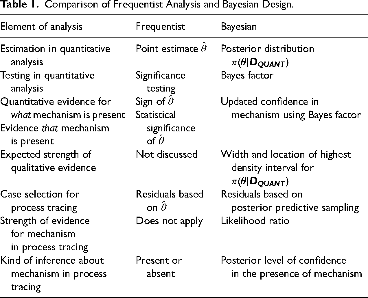
Comparison of Frequentist Analysis and Bayesian Design.

Element of analysis	Frequentist	Bayesian
Estimation in quantitative analysis	Point estimate $\hat{\theta }$	Posterior distribution $\pi (\mathit{\theta }|D_{QUANT})$
Testing in quantitative analysis	Significance testing	Bayes factor
Quantitative evidence forwhat mechanism is presentEvidence that mechanismis present	Sign of $\hat{\theta }$	Updated confidence inmechanism using Bayes factor
	Statistical significanceof $\hat{\theta }$
Expected strength of qualitative evidence	Not discussed	Width and location of highest density interval for $\pi (\mathit{\theta }|D_{QUANT})$
Case selection forprocess tracingStrength of evidencefor mechanismin process tracingKind of inference aboutmechanism in process tracing	Residuals based on $\hat{\theta }$	Residuals based on posterior predictive sampling
	Does not apply	Likelihood ratio
	Present or absent	Posterior level of confidencein the presence of mechanism

The stylized workflow in Figures 1 and 2 starts with a large-n analysis (as by Lieberman, 2005). The analysis can be implemented as a single-phase analysis, whereby each method is used once, or as a multiphase study with iterations of one or both methods. We discuss the Bayesian analysis as a multiphase design in which both methods inform each other in an iterative process. In the Concluding section, we briefly address designs starting with small-n research.

Figure 2.

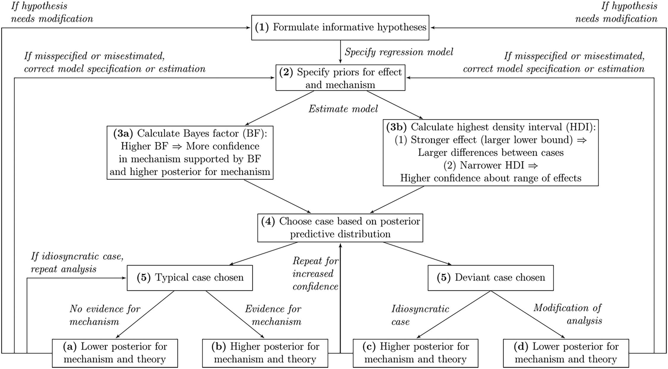
Procedure for Bayesian mixed-methods research starting with the quantitative analysis.

We introduce versions of Bayes’ theorem for the quantitative and qualitative analysis to lay the foundation for a detailed presentation of the design and workflow. Theorem 1 is used to make inferences about $\mathit{\theta }$ in the quantitative analysis. We refer to the quantitative data used in the regression analysis as $D_{QUANT}$ to distinguish it from the qualitative data $D_{QUAL}$ (process observations) collected in process tracing. The quantitative data can be of any kind and structure because the Bayesian design is open for different estimation approaches in the quantitative analysis (such as ordinary least squares (OLS) and generalized least squares (GLS)).

$$\pi (\mathit{\theta }|D_{QUANT})=\frac{f(D_{QUANT}|\mathit{\theta })\pi (\mathit{\theta })}{\int f(D_{QUANT}|\mathit{\theta })\pi (D_{QUANT})d\mathit{\theta }}.$$

(1)The prior distribution over the effect, $\pi (\mathit{\theta })$ , attaches a probability to each possible value that $\mathit{\theta }$ can take. The likelihood function $f(D_{QUANT}|\mathit{\theta })$ estimates how likely it is to observe the estimate $\hat{\theta }$ , given the assumption that $\mathit{\theta }$ takes a specific value. The prior distribution and likelihood function are the basis for deriving the posterior distribution $\pi (\mathit{\theta }|D_{QUANT})$ .

Theorem 2 presents the discrete version of Bayes’ theorem as it s used for process tracing (Abell, 2009; Beach and Pedersen 2019; Fairfield and Charman, 2017). ⁸ Following Lange’s argument, we use the negative mechanism ${\mathit{M}}_{\mathit{N}\mathit{E}\mathit{G}}$ for illustration. The formulation of a discrete prior for the mechanism, $p({\mathit{M}}_{\mathit{N}\mathit{E}\mathit{G}})$ , represents the researcher’s belief that ${\mathit{M}}_{\mathit{N}\mathit{E}\mathit{G}}$ was present. The likelihood for qualitative data is $\mathcal{L}(D_{QUAL}|{\mathit{M}}_{\mathit{N}\mathit{E}\mathit{G}})$ and tells us how likely it is to obtain an observation if ${\mathit{M}}_{\mathit{N}\mathit{E}\mathit{G}}$ is present. The prior and likelihood are needed to calculate the posterior $p({\mathit{M}}_{\mathit{N}\mathit{E}\mathit{G}}|D_{QUAL})$ based on the collected evidence. The Bayesian mixed-methods design is indifferent with regard to what variety of Bayesian process tracing is realized. It can be implemented with quantified parameters, or informally using linguistic qualifiers (see for a discussion, Abell, 2009; Fairfield and Charman, 2017; Zaks, 2017, 2020). Regardless of the formal-informal dimension, causal inference in process tracing can follow a difference-making perspective or a non-difference-making approach (Rohlfing and Zuber, 2021; Runhardt, 2022). This shows that the Bayesian mixed-methods design is flexible with regard to the process tracing approach that is used. ⁹

$$p({\mathit{M}}_{\mathit{N}\mathit{E}\mathit{G}}|D_{QUAL})=\frac{\mathcal{L}(D_{QUAL}|{\mathit{M}}_{\mathit{N}\mathit{E}\mathit{G}})p({\mathit{M}}_{\mathit{N}\mathit{E}\mathit{G}})}{p(D_{QUAL})}.$$

(2)We use the two theorems to elaborate on the workflow. In the main text, we focus on the components that are specific to the Bayesian design: the specification of priors (Stage 2); the calculation of the Bayes factor and the posterior highest density interval as two quantitative elements that inform process tracing (Stages 3a and 3b); and the choice of cases using posterior predictive sampling (Stage 4).

Our focus will be on typical (well-predicted cases based on the regression estimates) and deviant cases (badly predicted cases). Our concern with these two types of cases follows the discussion of nested analysis (Lieberman, 2005). We do not deal with extreme cases (Galvin and Seawright, 2023; Seawright, 2016a) and pathway cases (Gerring, 2007; Weller and Barnes, 2016), or other types in this article. We made this decision for three reasons. First, the answer to the questions as to what type of case to choose and how to do so is independent of the answers to the first two questions. The relevance of large parts of our arguments does not depend on how one answers the third question. Second, nested analysis with its focus on typical and deviant cases has guided the implementation of many empirical mixed-methods studies that choose either typical or deviant cases, or a combination of the two (see Supplemental Appendix Section C.1). Following this review, extreme and pathway cases do not seem to be used formally in mixed-methods research so far. This makes a Bayesian procedure for typical and deviant cases seem more relevant for empirical multimethod research. ¹⁰ Third, we see no reason why extreme and pathway cases are fundamentally incompatible with a Bayesian template. We leave it to a follow-up study to explore how other types can be integrated into Bayesian mixed-methods designs. We discuss additional elements of the workflow in the Supplemental Appendix: the formulation of informative hypotheses (Stage 1); the specification and estimation of the regression model (transmission from Stage 1 to Stage 2); the consequences of process tracing insights for updating the mechanism-related priors and the entire analysis if one realizes a multiphase study (Stage 5).

Stage 2: How Probable Effects and Mechanisms Are Ex ante: The Priors

In Stage 1, one starts with the formulation of hypotheses about theoretically possible effects and mechanisms. In the second stage, one has to specify a prior distribution ${\mathit{\pi }}_{\mathit{\theta }}$ for the effect and priors $\mathit{p}\mathbf{(}{\mathit{M}}_{{\mathit{\theta }}_{\mathit{d}}})$ for as many mechanisms as one wants to theorize and cover in the empirical analysis. For the effect, we specify the prior mean and prior variance for normal, Gaussian priors because they are conjugate priors for the likelihood function used in the linear regression that is central to our example. The prior mean is the effect size that a researcher believes to have the largest ex ante probability of equaling $\mathit{\theta }$ . The prior variance signifies our degree of confidence that $\mathit{\theta }$ is equal to the prior mean. The smaller the variance, the more confident we are that the prior mean equals the effect of $\mathit{X}$ .

The repertoire of strategies for the prior specification are the same in Bayesian multimethod research as in a standalone Bayesian regression and process tracing. First, the posterior of one empirical study is the prior of the next Bayesian study addressing the same research question (posterior passing, Brand et al., 2017). Second, one can use qualitative evidence for informed arguments about a plausible prior mean and variance. Third, this informal step can be formalized by relying on a structured evidence synthesis such as a meta-analysis or systematic reviews (van Grootel et al., 2020). Fourth, expert interviews can be used for prior elicitation. Regardless of the strategy one follows, which can possibly be in combination with other techniques, the rule of thumb is that the prior distribution for $\mathit{X}$ and the prior for the associated mechanism should reflect the respective state of knowledge. Dependent on the research question, one might be more confident in the effect of a variable than in the presence of a given mechanism, and vice versa. We do not aim to resolve or to add to the debate about prior specification because Bayesian mixed-method research serves a different purpose. In the “Illustration: British Rule and Colonial Development” section, we illustrate how published quantitative results can be used to specify priors. We further illustrate how to perform posterior passing within a single analysis, which reduces prior sensitivity, and realize a robustness test of the Bayesian estimates to the prior distribution (Supplemental Appendix Section E.3).

The specification of the regression model and prior distributions are the foundation for estimating the model as an intermittent step between Stages 2 and 3. In Stage 3, we use the regression results for addressing the first two questions, where the order does not matter. The inferences that one makes in the two steps need to be evaluated together to determine what mechanism one can expect to be present with what level of confidence (3a), and how much of a difference in within-case evidence we can expect to observe between two cases (3b).

Stage 3a: How Much More Confident One Can Be in a Mechanism and With What Level: The Bayes Factor

The overall question of what the regression results imply for the level of confidence in the presence of a mechanism has two theoretical and two practical components that are all related to the forward-passing of information from the quantitative to the qualitative analysis. First, how much do the regression estimates for $\mathit{X}$ change the level of confidence that one has in the presence of a specific mechanism. Second, what is the updated, posterior level of confidence in the presence of a mechanism? The practical questions concern the decision about whether resources (time, attention, and money) should be spent on finding evidence for one mechanism or multiple mechanisms.

We explain how one can address these four elements through a combined analysis of the Bayes factor (BF) and the credibility of the causal inferences about the effect of $\mathit{X}$ . We refer to the BF comparing the hypothesis of a negative and positive effect as $B{F}_{NEG/POS}$ and calculate it with the following equation:

$$B{F}_{NEG/POS}=\frac{m(D_{QUANT}|{\mathit{\theta }}_{\mathit{N}\mathit{E}\mathit{G}})}{m(D_{QUANT}|{\mathit{\theta }}_{\mathit{P}\mathit{O}\mathit{S}})}=\frac{\pi ({\mathit{\theta }}_{\mathit{N}\mathit{E}\mathit{G}}|D_{QUANT})/\pi ({\mathit{\theta }}_{\mathit{N}\mathit{E}\mathit{G}})}{\pi ({\mathit{\theta }}_{\mathit{P}\mathit{O}\mathit{S}}|D_{QUANT})/\pi ({\mathit{\theta }}_{\mathit{P}\mathit{O}\mathit{S}})}.$$

(3)The BF is the updating factor that expresses how much the data move our belief that the effect is negative rather than positive (Gill, 2015). We use established procedures of formal Bayesian hypothesis evaluation to calculate BFs (Kass and Raftery, 1995). The difference between the prior and the posterior distribution expresses the degree to which the data favor a negative effect over a positive effect, or the other way round (see Supplemental Appendix Section D.3.3). Figure 3 presents two hypothetical scenarios that illustrate different BFs with different implications for the qualitative analysis. Each panel contains the prior and posterior distribution and the likelihood function that accounts for the change from the prior to the posterior.

Figure 3.

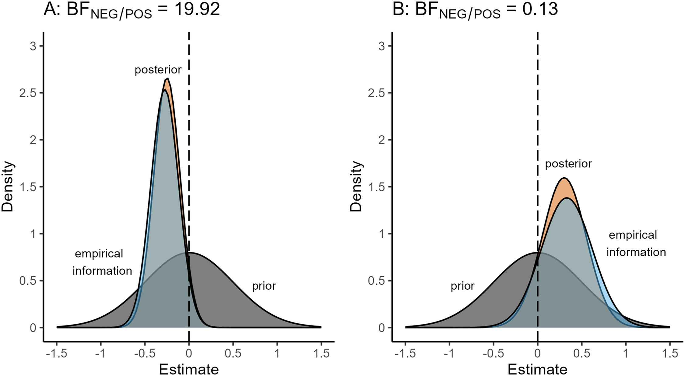
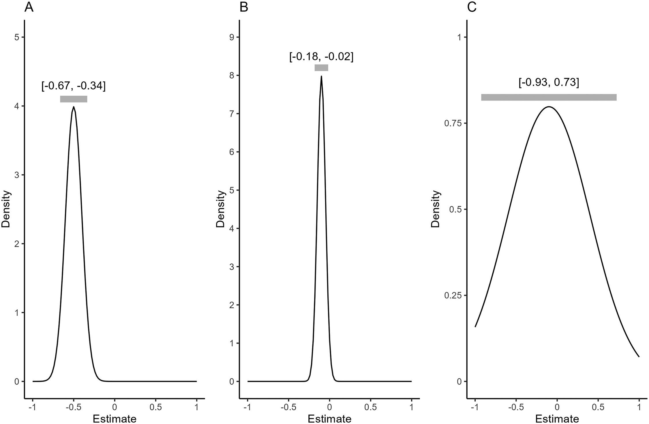
Strength of evidence for hypothetical pairs of prior and posterior distributions.

In Panel A of Figure 3, the likelihood function expresses a high level of confidence in a negative effect, with most support for an effect of $-$ 0.27. The resulting $B{F}_{NEG/POS}$ of 19.92 means that it is about 20 times more likely to estimate $\hat{\theta }$ when we assume that the effect of indirect rule is negative rather than positive. A factor of 20 can be interpreted as strong evidence with two implications for process tracing. ¹¹

First, we use the BF to update the priors for the negative and positive mechanisms. When the BF strongly indicates a negative effect of the degree of indirect rule, one can take this result and plug it into the ${\mathit{X}}_{{\mathit{\theta }}_{\mathit{d}}}\to {\mathit{M}}_{\mathit{d}}$ scheme. With a BF of 20, one should become more confident that the negative mechanism ${\mathit{M}}_{\mathit{N}\mathit{E}\mathit{G}}$ is present because the quantitative data strongly suggests the effect is negative rather than positive. This means that after the mechanism prior ${\mathit{M}}_{\mathit{N}\mathit{E}\mathit{G}}$ has been specified on ground of theory and empirical findings in Stage 2 of the analysis, it is updated in Stage 3 by incorporating the quantitative findings (see Supplemental Appendix Section D.3).

If one theorizes that multiple mechanisms could underlie an effect in the same direction, the BF is not informative about which of these mechanisms is more likely to be present. This is not a shortcoming of the BF, but follows from a generic ambiguity concerning which mechanism or mechanisms support this effect. The possibility of multiple underlying mechanisms for the same type of effect is the reason that one does mixed-methods research and uses process tracing. ¹²

The natural follow-up question for a BF of 20 is: How much should one update the priors of the mechanism based on the BF? For Panel A of Figure 3, does a BF of 20 mean that we should update the prior of the negative mechanism by a factor of 20? We argue that the BF alone is insufficient for answering this question because it does not capture whether the effect of $\mathit{X}$ is causal for $\mathit{Y}$ . If the BF was very large, but the effect not causal, for example, because of confounding, then one should not become more confident in the presence of a causal mechanism because the relationship ${\mathit{X}}_{\mathit{N}\mathit{E}\mathit{G}}\mathbf{\to }{\mathit{M}}_{\mathit{N}\mathit{E}\mathit{G}}$ does not exist.

This should be taken into account by factoring in the credibility of the quantitative causal inferences. The degree of credibility or trustworthiness of the inference that $\mathit{X}$ has a causal effect directly depends on the overall quality of the analysis up to the transition from the quantitative to the qualitative part. The interpretation of an estimate as causal depends on whether the identification and estimation assumptions that need to be met are fulfilled. This includes the familiar elements that may undermine the interpretability of the results, such as the formulation of hypotheses; conceptualization; measurement; operationalization; and the choice of the estimation approach. The greater the confidence that all assumptions and quality criteria of quantitative research are met, the higher the confidence that the BF is informative about the causal effect of $\mathit{X}$ on $\mathit{Y}$ and that it can be used to update the priors for the causal mechanisms. The views on what a problem of the analysis is, how much of a problem it is and how it should influence the credibility assessment needs to be decided by an empirical researcher for the study at hand. Every researcher has to make the potential problems and how they inform the assessment transparent. ¹³

The level of trust in the credibility of the quantitative causal inferences can be used as an adjustment or discount factor in the updating process for the qualitative priors. ¹⁴ For our example, it is plausible that the measure for “degree of indirect rule,” the share of customary court cases (Lange, 2009), exhibits systematic measurement error because the documentation of court cases could be more incomplete in more indirectly ruled colonies if they had weaker legal-administrative capacity. The possibility of systematic measurement error and, consequently, a biased estimator should decrease the level of trust in the causal interpretability of the estimate. ¹⁵ The consequence is that one increases the prior for the negative mechanism and reduces the prior for the positive mechanism less than a $B{F}_{NEG/POS}$ of 20 suggests. This shows that the qualitative analysis starts with mechanisms priors $p(M_d)$ that areinformed by theory about the mechanisms and by the BF and the credibility assessment of the quantitative analysis.

The second implication of the BF concerns the question of how widely to “cast the net” in process tracing and be open for finding evidence for different mechanisms (Bennett, 2015). The more the BF favors a negative over a positive effect, the more process tracing should focus on ${\mathit{M}}_{\mathit{N}\mathit{E}\mathit{G}}$ . A larger value of $B{F}_{NEG/POS}$ makes us increasingly confident that the effect is negative and that the associated mechanism is present, which justifies giving more attention to finding evidence for this mechanism. ¹⁶ The flip side is that the closer the BF is to 1, the less the quantitative data support the conclusion that $\mathit{X}$ works in one direction rather than the other. The weaker the quantitative data, the more process tracing may benefit from being exploratory and open to searching for evidence for mechanisms that underlie effects working in different directions that may offset each other in a quantitative analysis.

This use of the BF has implications for the distinction between a confirmatory, model-testing small-n analysis (mt-sna) and an exploratory, model-building analysis (mb-sna) that is salient in nested analysis (Lieberman, 2005). In the original formulation, a good model fit suggests adopting mt-sna focusing on one variable; an unsatisfactory fit requires the implementation of an exploratory mb-sna. In a Bayesian design, the BF as a continuous measure allows one to drop the crisp distinction and to decide about the approach based on the degree of confidence in finding evidence for ${\mathit{M}}_{\mathit{N}\mathit{E}\mathit{G}}$ rather than ${\mathit{M}}_{\mathit{P}\mathit{O}\mathit{S}}$ . The more the BF deviates from 1, the more one can justify the realization of mt-sna, and vice versa.

Stage 3b: What Strength of Process Evidence One Can Expect: The Posterior Highest Density Interval

The goal of process tracing is to find process observations that strongly support the presence of one mechanism and are unlikely to be collected under an alternative mechanism (Beach and Pedersen, 2019; Bennett, 2015). We show how one can use the posterior distribution for $\mathit{X}$ to supplement this goal by deriving expectations about the strength of process evidence. The posterior distribution $\pi (\mathit{\theta }|D_{QUANT})$ can be used to estimate the highest density interval (HDI), defined as the range of effects within which the effect of $\mathit{X}$ falls with a certain probability. For example, the 90% HDI is the part of the posterior distribution that covers the true effect of $\mathit{X}$ with a probability of 90%. ¹⁷ The location and width of the HDI together inform the qualitative analysis by representing the uncertainty about the range of possible effects, which has implications for the expected strength of process evidence.

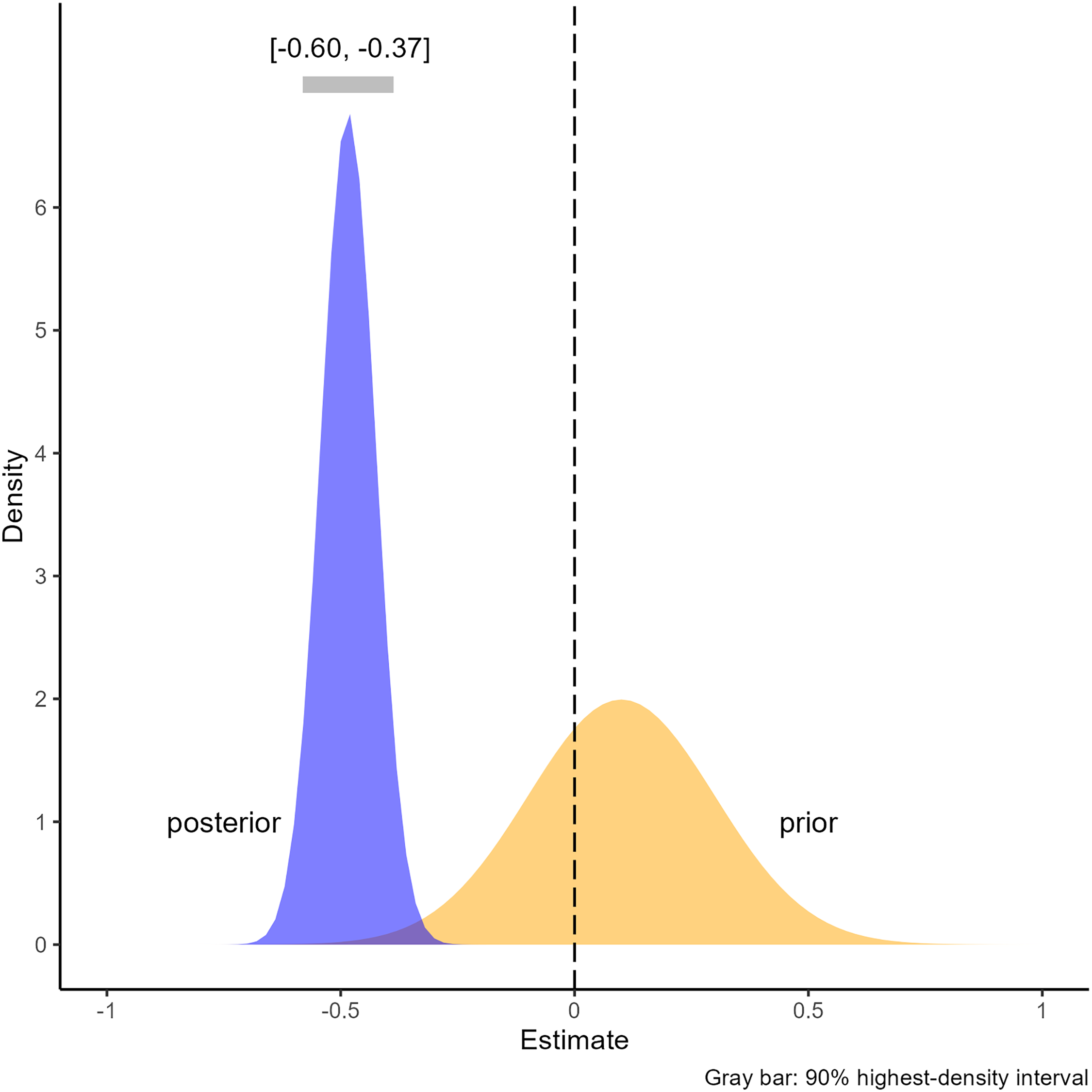
We illustrate the role of the HDI in Figure 4, presenting three hypothetical posterior distributions. In each panel, the gray bar represents the 90% HDI. The HDI in Panel A of Figure 4 ranges from $-$ 0.67 to $-$ 0.34, with a mean of $-$ 0.5. The HDI in Panel B of Figure 4 ranges from $-$ 0.18 to $-$ 0.02 and has a mean of $-$ 0.1. For Panel C of Figure 4, the 90% most probable effects range from $-$ 0.93 to 0.73 with a mean of $-$ 0.1.

Figure 4.

Three hypothetical posterior distributions with 90% highest density interval (HDI) (I-axis varies).

For Panel A of Figure 4, a 90% probability that the effect is between $-$ 0.67 and $-$ 0.34 allows one to infer that the effect of $\mathit{X}$ is negative and large because the lower bound is substantively different from 0. ¹⁸ Moreover, the HDI shows that the effect is precisely estimated with a range of about half a unit. We illustrate the implication of the HDI with one possible observable implication of the negative mechanism for the outcome “school attendance rate” (see “Illustration: British Rule and Colonial Development” section). One observable implication is that school budgets are larger in more directly ruled colonies. The school budget is a measure of fiscal bureaucratic capacity and should be positively related to the quality of the school infrastructure, the number of teachers that can be hired, and other measures of quality. A higher school budget should make a positive contribution to the school attendance of children. The observable implication of lower budgets under more indirect rule is very unlikely for the mechanism that underlies a hypothesized positive effect of indirect rule. If more indirect rule would be positive for development, one would expect that school budgets increase rather than decrease with an increasing degree of indirect rule.

When one infers that the estimated effect of indirect rule is large and negative, the expectation would be that the increase in indirect rule causes a correspondingly large decrease in the school budget. This expectation builds on a proportionality assumption between the effect size of “degree of indirect rule” and the difference between the process evidence of two cases that vary in their degree of indirect rule. When one infers from a quantitative analysis that the effect is large and negative and plugs ${\mathit{X}}_{\mathit{N}\mathit{E}\mathit{G}}$ into the sequence ${\mathit{X}}_{\mathit{d}}\to {\mathit{M}}_{\mathit{d}}$ , then one can deduce that an increase in indirect rule should cause a large decline in the districts’ school budgets. For the second step of the sequence, ${\mathit{M}}_{\mathit{N}\mathit{E}\mathit{G}}\mathbf{\to }\mathit{Y}$ , one can derive the expectation that a large decrease of school budgets contributes to a strong decline in the districts’ school attendance rates. ¹⁹

The proportionality assumption is central to understanding how the HDI is related to the expected relative strength of process evidence. The relative strength of qualitative evidence is the ratio of the likelihood of one hypothesized mechanism to the likelihood of another mechanism. We refer to the likelihood ratio (LR) comparing the negative and positive mechanisms as $L{R}_{NEG/POS}$ (equation (4)). The more likely an observable implication or actual observation is under one theory compared to another, the more the LR differs from 1 as the value denoting ambiguous evidence. ²⁰ In the example of school budgets, the larger $L{R}_{NEG/POS}$ , the more the presence of a decreasing school budget supports the inference that the capacity mechanism is present rather than the positive mechanisms. ²¹

$$L{R}_{NEG/POS}=\frac{\mathcal{L}(D_{QUAL}|{\mathit{M}}_{\mathit{N}\mathit{E}\mathit{G}})}{\mathcal{L}(D_{QUAL}|{\mathit{M}}_{\mathit{P}\mathit{O}\mathit{S}})}.$$

(4)When one focuses on a given observable implication, such as the level of school budgets, the expected relative strength of process evidence depends on two factors. First, the proportionality assumption implies that it increases with an increasingly lower bound of the HDI. We address the link between the lower bound and within-case differences in more detail below when discussing Panels B and C of Figure 4. Second, the expected strength of evidence increases as the cases’ difference on $\mathit{X}$ increases. ²² In a comparison of two cases that differ by 5 units on the degree of indirect rule, we expect a somewhat smaller school budget for the more indirectly ruled case. For the same HDI and two cases that differ by 85 units in the degree of indirect rule, we expect to see a much larger decline in the school budget because the two cases differ more strongly in their input into the ${\mathit{X}}_{\mathit{d}}\mathbf{\to }{\mathit{M}}_{\mathit{d}}$ sequence. ²³

Panels B and C of Figure 4 present different HDIs to illustrate the implications of their location and width for the qualitative analysis. Compared to Panel A of Figure 4, the location of the HDI in Panel B of Figure 4 implies that the expected process evidence is weaker because the upper bound is much lower and the lower bound is practically indistinguishable from 0. Panel C of Figure 4 illustrates the importance of using the HDI instead of the point estimate. Based solely on the point estimate of $-$ 0.1, one would expect to find evidence for the negative mechanism that is of moderate strength. The expectations differ significantly when one works with the HDI because the lower bound suggests the effect is large and negative. In contrast, the upper bound indicates it is large and positive, which implies the possibility that the effect is null and that no systematic mechanism is present. In this situation, the process observations that one collects in the qualitative within-case analysis might help one in developing a more precise idea about the direction and size of the effect of $\mathit{X}$ (see Supplemental Appendix Section D.6).

Stage 4: The Classification and Choice of Cases: Posterior Predictive Sampling

The third interactive element is the regression-based classification and choice of cases. The classification of cases as typical and deviant proceeds in four steps using posterior predictive sampling. First, one takes the posterior distribution $\pi (\mathit{\theta }|D_{QUANT})$ and samples one value for each regression parameter from it. Second, the sampled values are plugged into the regression equation and the predicted outcome value are calculated for each case. This step accounts for parameter uncertainty. Third, one captures the uncertainty of the data process by resampling the value of the dependent variable for each case. Fourth, the three steps are repeated many times to produce a posterior predictive distribution (PPD) that represents the distribution of outcomes that are expected for each case under the model. Cases with an observed outcome that falls inside the 90% interval of the PPD are classified as typical because they are sufficiently well predicted (we use 90% for illustration). A case with an observed outcome in the upper or lower 5%-tail of the PPD are classified as deviant. ²⁴

In the next step, classification is the basis for case selection. The choice of a single typical or deviant case should be guided by the research question. For a typical case, the interest could be the collection of evidence for high state-administrative capacity in a directly ruled colony or for low capacity in an indirectly ruled colony. For a single deviant case, one could select an overperforming case that did unexpectedly well or an underperformer that shows a poorer outcome than was predicted. ²⁵ A comparative analysis of two typical cases follows the idea of a most-similar comparison wherein two typical cases differ in their degree of indirect rule and development and are similar on all other covariates. One should choose from the set of typical cases a diverse pair that maximizes the difference between $\mathit{X}$ and $\mathit{Y}$ . The larger the difference in the starting point and the end point of the ${\mathit{X}}_{\mathit{d}}\to {\mathit{M}}_{\mathit{d}}\to \mathit{Y}$ sequence, the stronger the process evidence should be and the easier to discriminate between competing mechanisms. ²⁶ For the comparison of a typical case and a deviant case, we propose the comparison of two cases that are as similar as possible on all covariates and are as diverse as possible in their outcome values. Two cases that strongly differ in the outcome should also strongly differ in the values on the cause that is to be determined in exploratory process tracing. Following the proportionality assumption, the unknown cause should be easier to detect for cases that are diverse on $\mathit{Y}$ because they are also likely to strongly differ in their process observations. We illustrate the classification and choice of cases in the following section that applies the Bayesian design to the leading example.

Illustration: British Rule and Colonial Development

Quantitative Analysis

The original analysis uses the share of customary court cases in a colony as a proxy for the form of British rule (Lange, 2009). A higher share of customary court cases represents more indirect British rule, which is hypothesized to have a negative effect on five outcomes: GDP per capita (2000, log); average school attainment (1995); infant mortality rate (2000) ²⁷ ; aggregate quality of governance (1996–2005); and average level of democracy (1972–2005) (Lange, 2009). The five outcomes are alternative measures of development and are neither theoretically nor substantively important in themselves. We can exactly reproduce the frequentist estimates for the five original OLS models using the original data (see Supplemental Appendix Reproduction Material).

We have introduced the hypotheses on the negative effect and negative mechanism in the “Empirical Example” section (Step 1 of the workflow). In Stage 2, we must specify the priors for all variables in the regression model and the mechanisms. The use of five outcomes in the quantitative analysis allows us to implement posterior passing. Posterior passing means to pass forward information within the quantitative stage by using the posteriors of one regression analysis as the priors for the next (Brand et al., 2017). Posterior passing makes the most of the estimates of one analysis by conveying information from one model to the next. Posterior passing has two implications for the Bayesian regression. First, we only need to review existing research to specify the priors of the first model that we estimate because it produces priors for the second model, and so on. Second, a practical requirement is that we need to standardize all variables to estimate effects using a common scale.

We start posterior passing with the outcome “GDP/capita” and finish with the outcome “level of democracy.” “GDP/capita” is the first outcome because a review of colonialism research shows that it offers the most results on which to build. Our review is based on the literature that had been available at the time the original analysis was done (see Supplemental Appendix Section E.2). With regard to the form of rule, multiple studies have found that British rule had a positive effect on development and economic growth, as compared to French and Spanish colonial rule. This is indicative of a positive marginal effect of indirect rule because British colonies are consistently described as having been more indirectly ruled (Bernhard, Reenock, and Nordstrom, 2004; Brown, 2000; Grier, 1999: section 2). We use this evidence to specify a prior for the degree of indirect rule that expresses a moderate level of confidence in a positive effect with a mean of 0.1 and a standard deviation of 0.2. ²⁸ The hypothesized capacity mechanism is tied to a negative effect of indirect rule. Based on the expectation that a positive effect is more likely than a negative effect, we assign an informally specified low prior $p({\mathit{M}}_{\mathit{N}\mathit{E}\mathit{G}})$ to the negative mechanism. ²⁹

The reviewed research further indicates that two control variables (see Lange, 2009), latitude (Acemoglu, Johnson, and Robinson, 2001) and ethnic fractionalization (Bernhard, Reenock, and Nordstrom, 2004), have a negative effect on development. We assign a prior mean of $-$ 0.1 and standard deviation of 0.2 to each variable. We assign a mean of 0 and standard deviation of 100 to the other variables for which we could not find estimates to build on. ³⁰ Using these priors for the first model, the posterior estimates are passed forward four times in this order of outcomes: GDP/capita $\to$ average school attainment $\to$ infant mortality rate $\to$ quality of governance $\to$ level of democracy. Except for the first outcome, there is no specific reason for the order. The order does not matter for the final posterior distribution, the BF and the HDI. ³¹

In the transition from Stages 2 to 3, we estimate each model with a normal likelihood function and conjugate normal priors using Hamiltonian Monte Carlo sampling (Gill, 2015: section 15.4). We begin with two separate Markov chains and check the results for convergence using the Gelman-Rubin diagnostic (Gill, 2015). For each model, the estimates are based on one chain and 10,000 posterior draws, from which we exclude the first 2,000 as warm-ups. We present the complete results for the final model in Supplemental Appendix Section E.4 and focus on the implications for the interactive elements of the design.

Implications of Estimates for Qualitative Analysis and Case Selection

We present the prior and posterior distributions for the final model that serves as the basis for Stages 3a and 3b (Figure 5). The 90% HDI ranges from $-$ 0.6 to $-$ 0.37 with a mean of about $-$ 0.49. This is a substantively large estimate with a narrow interval. Following the proportionality assumption, the HDI lets us expect to find strong evidence for the negative mechanism in an analysis of two typical and diverse cases.

Figure 5.

Prior and posterior distributions for degree of rule.

The BF shows that the quantitative data very strongly favor a negative over a positive effect with a natural log of the $B{F}_{NEG/POS}$ of about 38. ³² Two analysis-related factors suggest that we should be more moderate in updating the mechanism priors than the high value of $B{F}_{NEG/POS}$ suggests. First, it is possible that the adjustment set of covariates in the regression analysis does not allow one to identify the effect of degree of indirect rule. The percentage of European settlers would be a mediator of “degree of indirect rule” if European settlers had a higher settlement propensity in more directly ruled colonies, for example, because they wanted to benefit from a stronger infrastructure. If true, the analysis would suffer from post-treatment bias for the total effect (Keele at al., 2020). Process tracing could focus on this and other identification assumptions to validate the adjustment set or suggest how to correct it (Lieberman, 2005; Seawright, 2016b: chapter 3).

Second and building on what we discussed in the “Stage 3a: How Much More Confident One Can be in a Mechanism and With What Level: The Bayes Factor” section, the share of customary court cases as the measure for degree of indirect rule might exhibit non-systematic and systematic measurement error. When we factor in these limitations, we find it appropriate to update the low prior $p({\mathit{M}}_{\mathit{N}\mathit{E}\mathit{G}})$ only to a moderately high level. This level is high enough to justify a strong focus on the negative mechanism in process tracing and to largely follow the template of a model-testing small-n analysis.

For the classification of cases in stage 4, we calculate 1,000 predicted outcome values and derive the 90% prediction interval (PI) for each case. ³³ Figure 6 plots the mean predicted values and 90% PIs against the observed outcomes. The plot shows that 35 cases are classified as typical and that four cases are deviant. ³⁴

Figure 6.

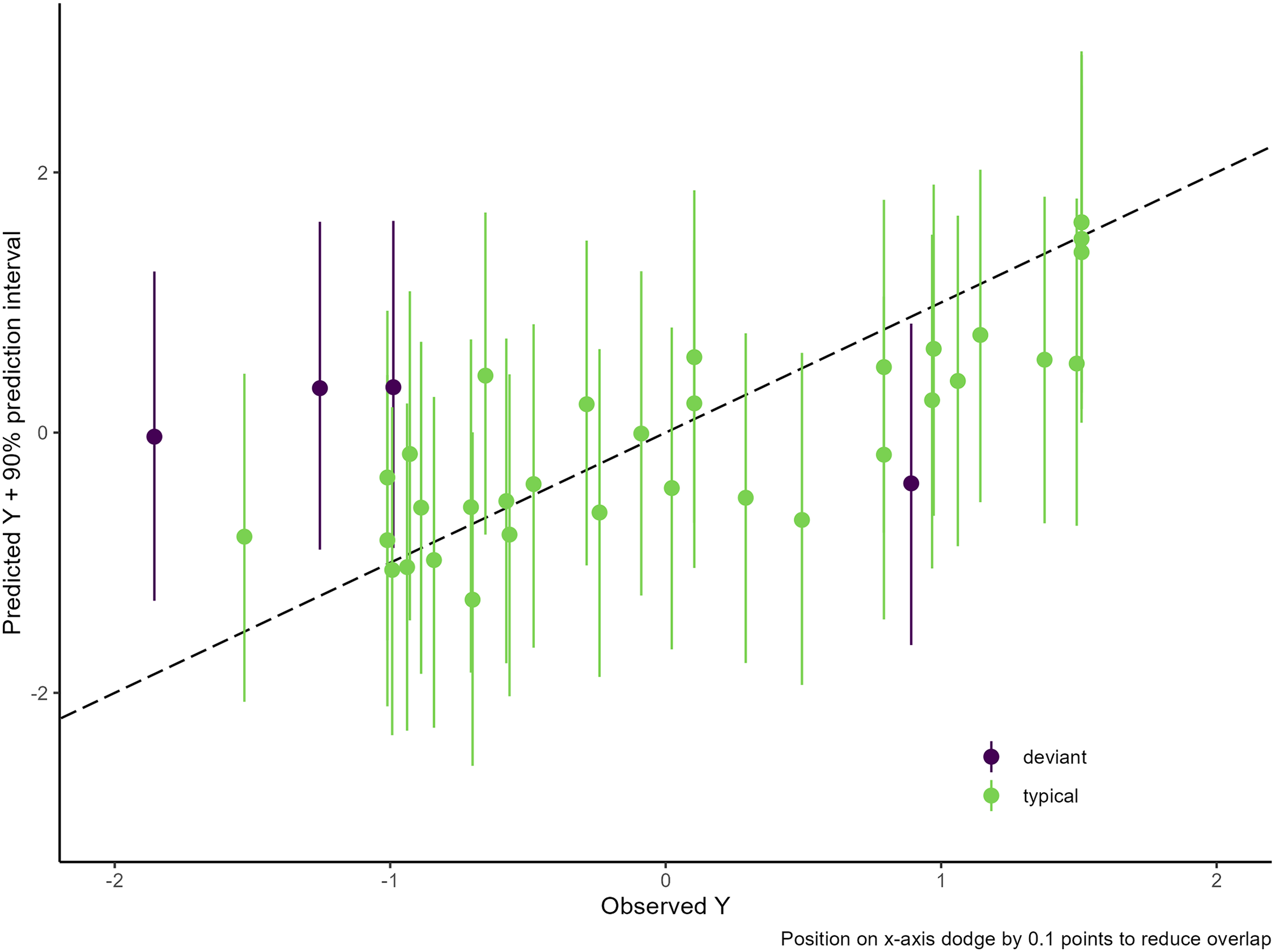
Predicted-versus-observed plot based on the final model.

Based on their classification, we choose cases for comparative process tracing following the idea of a most-similar design based on the calculation of their distances on the outcome, the degree of indirect rule and the set of controls. ³⁵ For each pair of typical cases, we plot the difference in the level of democracy against the difference in the degree of indirect rule (Figure 7). The size of the marker symbols is proportional to the distance of the pair on all control variables in the regression analysis. There is no ideal pair of typical cases that combines the maximum distance in the degree of indirect rule and the level of democracy with a minimal distance on the controls. ³⁶ If this holds, which depends on the data at hand, one has to decide whether to trade off a larger distance in $\mathit{X}$ against a smaller distance in $\mathit{Y}$ or the controls, or if another kind of trade-off is preferable. For our data, a comparison of Nigeria and the USA would establish the maximum diversity on $\mathit{X}$ (93 points) and a large difference on $\mathit{Y}$ (5.685 points) at the expense of a moderate distance on the controls (about 801 points).

Figure 7.

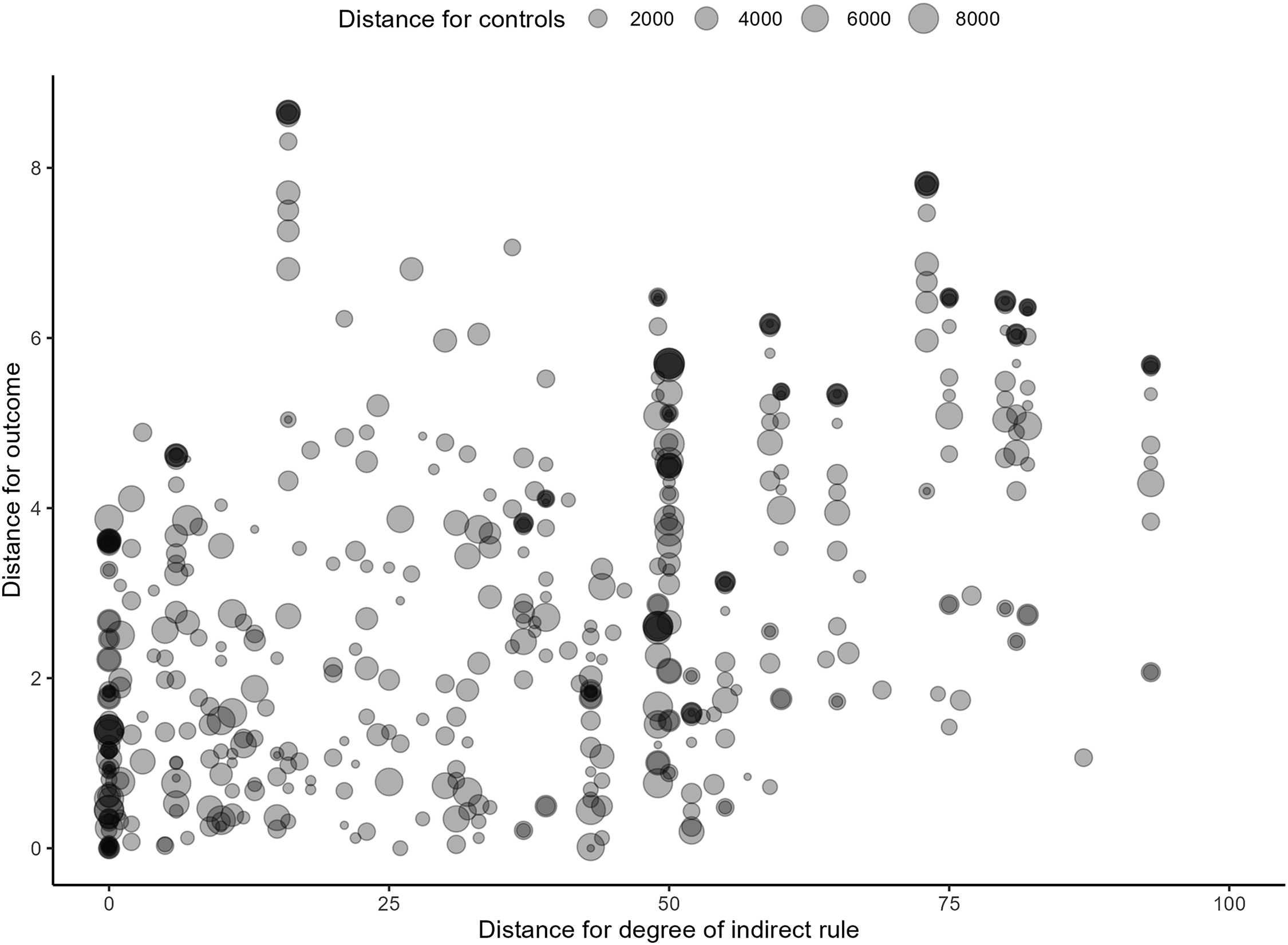
Similarity of pairs of typical cases.

The alternative is a comparison of Barbados with Malawi. The two countries differ in the degree of indirect rule (82) less than do Nigeria and the USA, but have a slightly larger difference on $\mathit{Y}$ (6.31 points) and reduce the distance on the controls by a factor of about eight to 107 points. The two pairs might not seem like natural candidates for comparison. They underscore the argument that formal regression-based choices promise a fresh perspective on case selection and comparisons (Lieberman, 2005).

Comparison with Other Mixed-Methods Approaches

Nested Analysis

We compare the quantitative-to-qualitative interaction between our design and a frequentist analysis to illustrate how the decisions and conclusions are made on a different basis and that, to some degree, the decisions differ substantively. In a nested analysis, for answering the question of what mechanism one can expect to be present and with what level of confidence, one would use the statistically significant, negative estimate of ‘degree of indirect rule'. The estimate is negative for all five outcomes, where one would not be able to implement posterior passing because this is not possible in a frequentist setup. This result would also lead us to expect that the negative mechanism is present, meaning that we would opt for mt-sna in a nested analysis and our Bayesian design. However, in a frequentist analysis, we would neither know how much more confident we can be nor what the updated level of confidence in the negative mechanism is because there is no conventional frequentist equivalent to the BF. The estimate for $B{F}_{NEG/POS}$ in the Bayesian analysis gives us more specific information and guidance for process tracing and integrates the quantitative and qualitative parts more closely with each other.

For a comparison of the expected strength of process evidence (Stage 3b), Figure 8 presents the prior distribution for “degree of indirect rule” and the five posterior distributions next to the frequentist estimates. They are arranged from bottom to top in the order that we estimate them for posterior passing. For each outcome, the HDI is smaller than the corresponding confidence interval (CI), which is the frequentist equivalent to the HDI. For the final outcome, the CI ranges from $-$ 0.91 to $-$ 0.06, which suggests that the effect in the population from which a sample was drawn could be large or could be close to zero and substantively negligible. The wide CI would leave us with a high level of uncertainty about the effect size and we would have to be open to the possibility of finding very strong, but also weak and practically negligible qualitative evidence. In contrast, with a range from $-$ 0.6 to $-$ 0.37, the HDI is estimated more precisely. The width and location of the HDI leads us to expect to find strong evidence for the negative mechanism and again gives us more precise guidance for process tracing.

Figure 8.

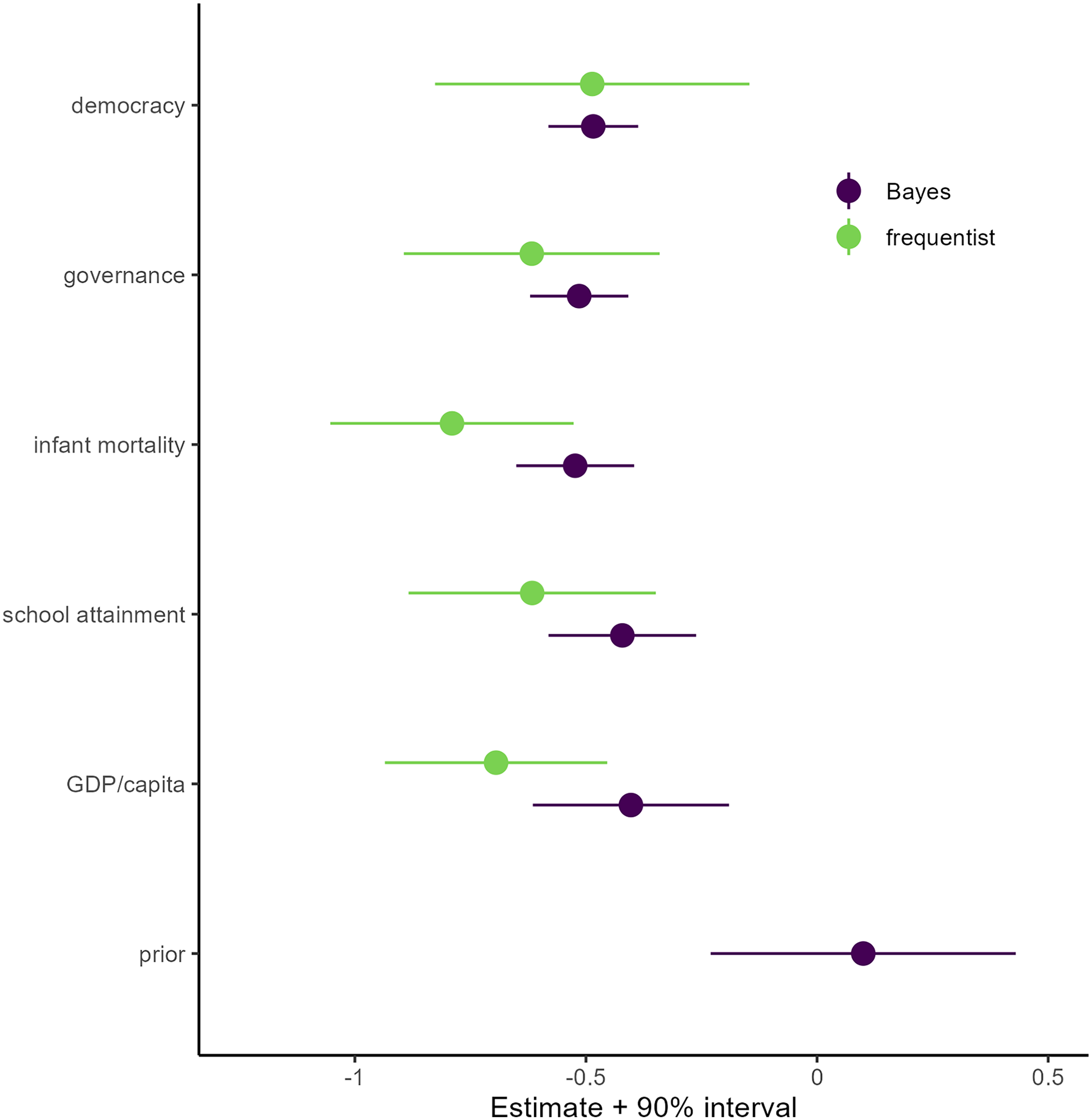
Estimates for effect of degree of rule.

For stage 4, we compare the classification of cases across all five models using the 90% PI (Figure 9). We focus on whether a case has the same status in nested analysis and a Bayesian analysis, as this step is fundamental for the choice of cases in the second step. The models are arranged from left to right in the order that we estimate them for posterior passing. The plots show that case classifications differ for four models out of five, whereas the number of cases that are classified differently is small for each model.

Figure 9.

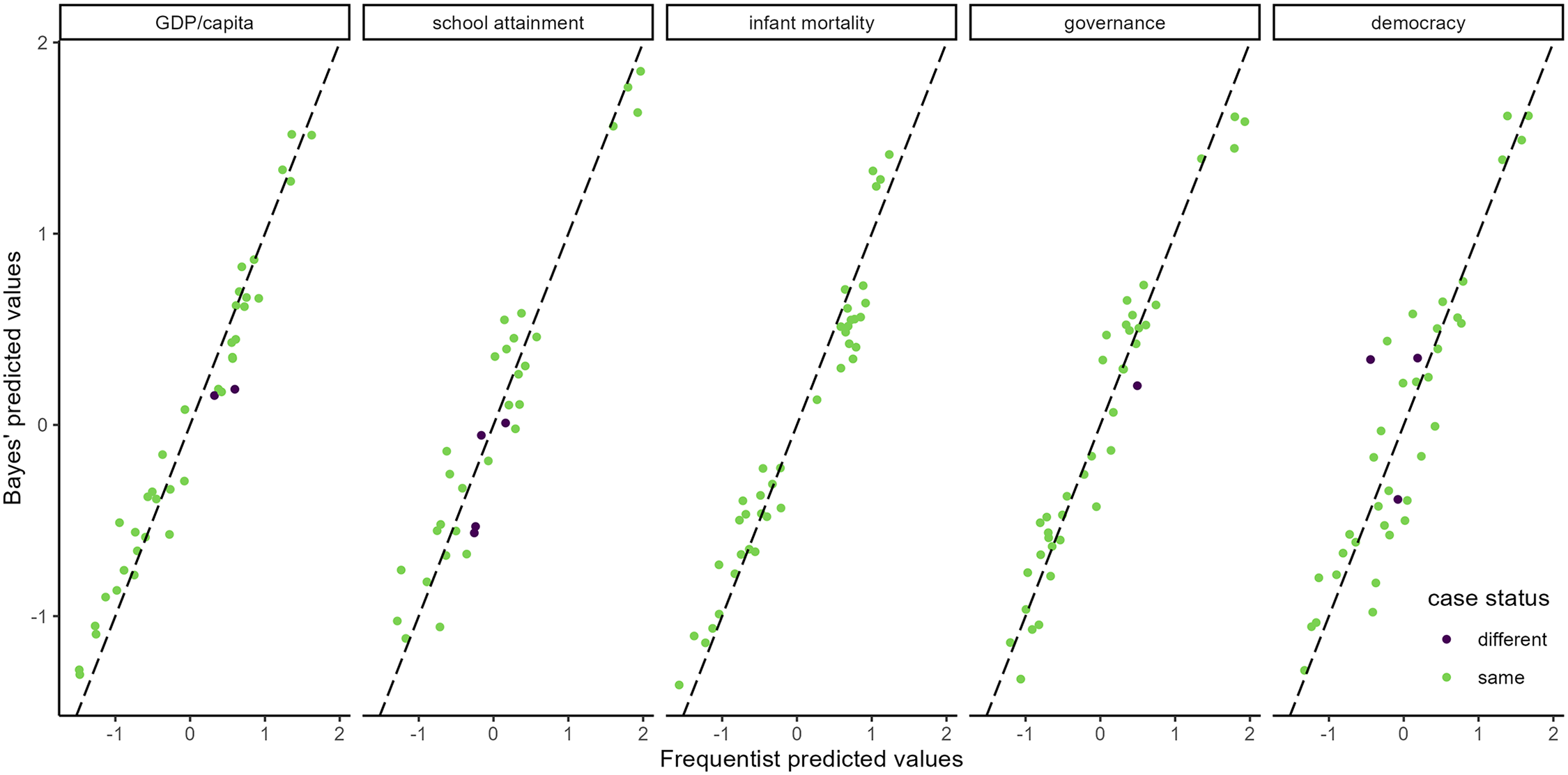
Comparison of case classification using 90% prediction intervals.

In summary, the illustrative comparison shows that the original frequentist analysis and a Bayesian analysis produce different quantitative results (beyond salient differences in their frequentist and Bayesian interpretation), which allows one to derive more informative expectations from the Bayesian regression estimates. The integration of quantitative and qualitative methods and sequential updating of priors are one advantage of the Bayesian design over the frequentist alternative. This means one should choose the Bayesian design when the goal is to quantify the uncertainty about what the possible direction of the effect and the underlying mechanisms are. We believe that the value of the Bayesian design is higher, the stronger the theory is that one can use to derive priors for the effect and mechanisms. This implies that the classic nested analysis may be preferable if theory is weak. In principle, one could work with flat priors in a Bayesian framework when theory is weak. However, one may still prefer the computationally and formally more lightweight frequentist approach to sharpen theory first and lay the basis for a follow-up Bayesian mixed-methods design.

We conclude the illustration by addressing two potential points of criticism. First, one might argue that the differences between a frequentist analysis and a Bayesian analysis are not large. Besides the fundamental differences in the interpretation of Bayesian and frequentist results, the similarities follow from the strong quantitative evidence for a negative effect of degree of indirect rule that dominates the prior information speaking for a positive effect. In Supplemental Appendix Section F, we present results of Monte Carlo simulations that show under what conditions a Bayesian analysis and nested analysis differ from each other in the interactive component of the design. The simulations show, first, that the differences in case classifications are the larger, the smaller the number of cases. Second, the results differ the more the prior information and information in the data diverge. Third, differences are larger whenthe weight of the prior information is larger, relative to the weight of the data. Of these three conditions, only one is met in our example because the sample size is small. The simulation results demonstrate that when all three conditions coincide, the differences between a Bayesian analysis and frequentist analysis are sizable.

Second, one might observe that the differences mainly derive from posterior passing, which is neither a necessary component of our design nor always available in a Bayesian mixed-methods study. The comparison of the Bayesian estimates with the results from the nested analysis show that they do not mainly follow from posterior passing. When one imagines that we only estimate one regression with GDP/capita as the outcome, the CI indicates an effect of indirect rule that is larger than the effect estimated with the HDI (CI: $-$ 0.94 to $-$ 0.45; HDI: $-$ 0.65 to $-$ 0.15). We would expect to collect weaker process evidence based on the HDI than on the CI. For case classification, the panels in Figure 9 further show that the designation of cases as typical and deviant is not identical after one estimation round. This reveals that posterior passing does not produce differences between the results that would be absent after a single regression analysis without posterior passing.

Integrated Inferences and the Bayesian Integration of Quantitative and Qualitative Evidence

The Bayesian integration of quantitative and qualitative evidence (BIQQ) is an alternative approach that uses cross-case and within-case data (Humphreys and Jacobs, 2015, 2023). In its present form, BIQQ works with a small number of binary variables, including the treatment, and a binary outcome. Its key strength is the simultaneous updating of beliefs about the effect on the cross-case level and the mechanism on the within-case level, implying that BIQQ belongs to the class of simultaneous mixed-method designs. Given the constraint that one has to work with binary variables, this approach should be particularly attractive for integrated cross-case and within-case analyses in causal qualitative research.

The approach that we propose belongs to the group of sequential mixed-method designs. At a given stage of the analysis, one either updates quantitative or qualitative beliefs that are forwarded to the next part of the analysis. Our framework uses regression analysis for the estimation of treatment effects. This gives researchers the flexibility to choose the regression approach that is needed for the data structure at hand without the need to dichotomize variables. The chosen estimation approach only needs to give a researcher the opportunity to distinguish different types of cases using an appropriate criterion. What this criterion is depends on the types of approach; for OLS regression, it is the residual of a case and a criterion that guides case classification (Rohlfing and Starke, 2013). For generalized linear models with a logistic link function, one can calculate predicted probabilities for each case and compare them with the observed outcome to distinguish well-predicted from not-so-well predicted cases. Similar criteria can be devised for other estimation approaches such as event-history analysis and regressions for count data. This shows that BIQQ and our Bayesian mixed-methods design are not substitutes, but complement each other. They are alternative approaches that one can choose from depending on the research goal and the nature of the data at hand.

Conclusion

We proposed a design and procedure for the integration of Bayesian regression with process tracing. Our discussion has been guided by the idea of mixed-methods research that starts with a regression analysis. Future work on Bayesian mixed-methods research could develop a design that starts with Bayesian process tracing and performs the regression analysis as a second step. In this version of a Bayesian mixed-methods study, it would be crucial to work out how the qualitative results could inform the specification of prior distributions for the regression parameters. A Bayesian “process-tracing first” design along these lines would be a valuable addition to the Bayesian mixed-methods toolbox. A second possibility for further development is the exploration of how alternative types of cases such as extreme cases and pathway cases could be defined and chosen in a Bayesian analysis.

Supplemental Material

sj-png-1-smr-10.1177_00491241241295336 - Supplemental material for The Integration of Bayesian Regression Analysis and Bayesian Process Tracing in Mixed-Methods Research

Supplemental material, sj-png-1-smr-10.1177_00491241241295336 for The Integration of Bayesian Regression Analysis and Bayesian Process Tracing in Mixed-Methods Research by Lion Behrens and Ingo Rohlfing in Sociological Methods & Research