
Abstract
To explain the inequalities in access to a discrete good G across two populations, or across time in a single national context, it is necessary to distinguish, for each population or period of time, the effect of the diffusion of G from that of unequal outcomes of underlying micro-social processes. The inequality of outcomes of these micro-social processes is termed inequality within the selection process. We present an innovative index of measurement that captures variations in this aspect of inequality of opportunity and is insensitive to margins. We applied this index to the analysis of inequality of educational opportunity by exploring the effects of the British 1944 Education Act, of which various accounts have been offered. The relationships between the measure of inequality within a selection process presented and classical measures of inequality of opportunity are analyzed, as well as the benefits of using this index with regard to the insight it provides for interpreting data.
Keywords
Introduction
The methodological problem at issue here arises in any field where comparing access to a discrete good, G, requires explanations of the social processes generating observed inequality, such as labor discrimination, schooling inequalities, social mobility, urban segregation, and so on.
When we account for situations of unequal access to a specific good G across two populations, or across time in a single national context, we need to differentiate the effect of social processes from the effect of margins—the distribution of social subgroups in the population and the overall rate of access to the good G—on the observed inequalities. In this respect, much has been written on the importance of margin insensitivity of indices in comparative studies, but there has been a tendency to confuse a measurement of inequality insensitive to marginal distributions with inequality of social processes irrespective of the margins’ role. A margin-insensitive index is independent of the value of the margins regarding the specific aspect of inequality it captures, while assessing inequality of social processes irrespective of the role of the margins relates to an aspect of inequality of opportunity that none of the conventional indices account for. To address this issue, we rely on the index of inequality developed by Bulle (2009), which permits a comparison of the results of the selection process for access to a discrete good G—that is, the outcomes of the micro-social processes that underlie access to G, irrespective of the opening up of access to G.
To support our argument, we use an example: an analysis of the effect of the British 1944 Education Act on inequality of access to a grammar school education. We compare the assessments provided by some conventional measures of inequality and illustrate the limitations of their accounts of the observed trends. We then outline the case for an alternative measurement method and present the measure developed by Bulle (2009). Next, we analyze the relationships between this measure and various indices of inequality of opportunity. Returning to the 1944 example, we show how using this new measurement method improves the analysis and provide an interpretation of the new results.
Measuring Inequality of Educational Opportunity: The Example of the British 1944 Education Act
The 1944 Act
From 1902, and for nearly half a century, pupil selection for secondary education in British schools was based on a competitive examination taken at the age of 11, with an important place given to intelligence tests. Pupils who passed the examination obtained a free place in a grammar school; pupils who failed the examination were only able to follow an equivalent course of studies in a private school. 1 The 1944 Education Act extended free education to all state secondary schools, raised the school-leaving age from 14 to 15 (effective from 1947), and introduced the tripartite system dividing the secondary system into three types of schools, namely, grammar schools, secondary modern schools, and secondary technical schools. The kind of secondary school education students received depended mainly on the results of the “11-plus” examination—which was similar to the old Special Place examination to which it replaced. Even if the 1944 Act is “widely regarded as a landmark of social change” (Blackburn and Marsh 1991:508) making free secondary education available to all, and also offering a greater number of free places in selective schools, the meritocratic selection process varied only slightly from the system it superseded. 2
The effect of these changes on the inequality of access to selective schools in England has been studied by a number of sociologists using various data sets, measures, and models. The pursuit of improvements in measurement tools has been unending, with the objective of understanding accurately the role in educational inequality of the main factors investigated here, that is, selection processes and the availability of places in selective schools.
Analyses of the Effects of the 1944 Education Act
In an article that is a standard reference on the issue, Little and Westergaard (1964) considered the evolution of inequality of access to lengthy secondary education (i.e., in grammar and independent schools) for English children in the first half of the twentieth century. Their data on boys’ and girls’ secondary schooling were derived from the following two sources: Floud’s (1954) analysis of a survey conducted in July 1949—a random sample of 10,000 English men and women aged 18 years and over (born before the Second World War)—and the Crowther Report’s (1959) sample of national service recruits (cf. Table 1). 3 Little and Westergaard offered a mixed account, pointing out that different results were obtained depending on whether the analysis was based on the chances of gaining access to a selective school—which were multiplied by 10 for children in the lowest social group but by 1.7 for those of the upper group—or on the risk of not gaining access to them—which reduced by nearly half for children from homes in the upper social group but by barely a tenth for children from the lowest social group. Everything depends, the authors concluded, on “the relative weight one attaches to the proportion achieving, as compared with the proportion who fails to achieve selective secondary schooling.” But, they explained, the effect of the 1944 Act on these inequalities was still not clear; the reduction of social inequalities that followed the Act was a continuation of a long-term, gradual trend.
Proportions in Different Classes Obtaining Education of a Grammar School Typea by Birth Cohort.
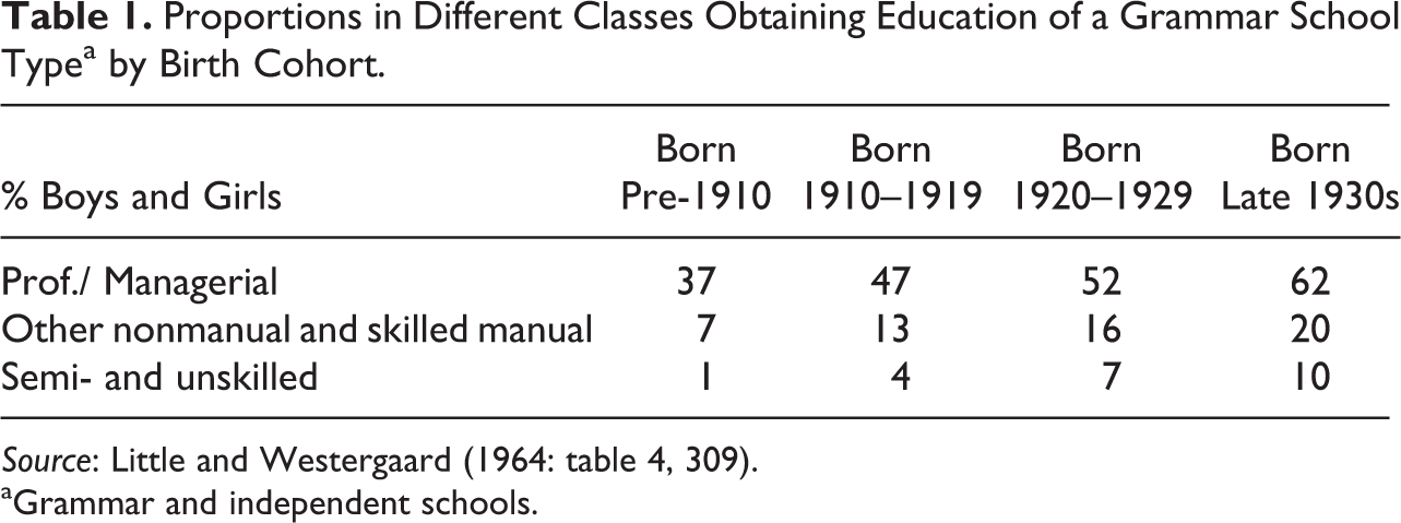
Source: Little and Westergaard (1964: table 4, 309).
aGrammar and independent schools.
Comparing data on the evolution of inequality of opportunity in different countries with the data for Great Britain published by Little and Westergaard—because such data provided a long-term picture of the evolutions at issue, Boudon (1974:143-58) made the assumption that a similar structural change occurred in the expanding educational systems of industrialized societies. This structural change in the inequality of opportunity underpins the general explanatory model of expansion of educational systems that Boudon developed. 4 Also referring to the data published by Little and Westergaard (1964:309), Combessie (1984) concluded that there was an irreducible diversity of accounts of inequality of opportunity, given the various foci of the measures used.
Blackburn and Marsh (1991) reopened the case, this time on the basis of data published by Halsey, Heath, and Ridge (1980), derived from the Oxford Mobility Study, a representative sample of English and Welsh men interviewed in 1972 (cf. Table 2) divided into four 10-year birth cohorts, two entering secondary education before the 1944 Act and two afterward. The original analysis was restricted to men between the ages of 20 and 59 who received their secondary education in England and Wales. Blackburn and Marsh noted that no clear conclusions about the effect of the 1944 Act itself were drawn by Halsey et al. and that, according to Heath’s words in subsequent works, the study showed that nothing had changed over the years. Blackburn and Marsh reconsidered the same data and compared accounts based on various measures of inequality, particularly the segregation index they developed, which is insensitive to marginal distributions: the marginal matching coefficient (MM).
Attendance of Boys at Selective Schoolsa by Class and Birth Cohort.
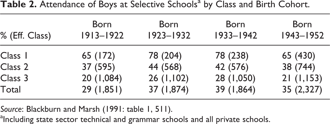
Source: Blackburn and Marsh (1991: table 1, 511).
aIncluding state sector technical and grammar schools and all private schools.
It should be noted that Blackburn and Marsh departed from Halsey et al. in their approach to class categorization. In the original analysis, respondents were assigned to one of the three classes on the basis of paternal occupation when the children were aged 14 years: a “service” class of professionals and managers at the top, a “working” class of manual workers at the bottom, and an “intermediate” class in between. Blackburn and Marsh recoded paternal occupations using an index of social advantage—based on social networks analysis—and then divided the occupational scale into class sizes within each 10-year cohort to produce the class margins reported by Halsey et al.
As shown in Table 2, the first three birth cohorts saw their access to selective forms of secondary education increase; but for the last, access declined as population growth outstripped the rise in places. Blackburn and Marsh noted that different classical measures of association between educational and social stratification give different accounts of the evolution of educational opportunity (see Table 3) for the top and bottom classes (given in Table 2). Looking at the ratio of proportions RP, educational opportunity diminished in the first three periods and rose in the last; according to the phi coefficient, Φ, opportunity rose throughout the period, whereas the odds ratio, Ω, and the difference of proportions, d, indicated that they rose initially, before falling after the Act.
Different Summaries of the Relationships between Class and Selection, for Classes 1 and 3, in the Four Cohorts.
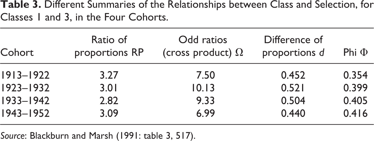
Source: Blackburn and Marsh (1991: table 3, 517).
If one wants to know what intrinsic changes in inequality of opportunity may have occurred, the problem is, as Blackburn and Marsh noted, how to disentangle such changes from the effects of variation in margins. Class size and school place margins constrain the range of RP, d, 5 and Φ. 6 Because there were more selective places than children in class 1 (as defined in Table 2), children from other classes had to be selected. Besides, the RP measure is incomplete because it only takes into account the selected and not the nonselected children. Using the cross product or odds ratio (Ω) 7 avoids these limitations: It takes both selected and nonselected children into account and is insensitive to margins variation.
As we will see in the next section, margin insensitivity notwithstanding, Ω cannot capture the changes in inequality of opportunity we are looking for to support explanation of the evolutions under consideration—that is, changes in inequality regarding the effect of the micro-social processes generating access to the good G at stake—for instance, a grammar school education—irrespective of the availability of places in grammar schools.
Measuring Inequality Within a Selection Process
The Issue of Margin Insensitivity
The degree of inequality of access to a discrete good G measured by an index that is insensitive to marginal distributions should not be limited either by the proportion of individuals in the population gaining access to G or by the relative size of the various social groups. Consequently, these proportions, or the relationships between these proportions, should not constrain the index values, such that in each context defined by the contingency table’s margins, the same degree of inequality may be observed. These conditions that exclude any structural artifact from the comparison of the degree of inequality in different social contexts are, of course, extremely restrictive.
For instance, we saw previously that chances of gaining access to a selective school were multiplied by 10 for children in the lowest social group and by 1.7 for those of the upper social group. But, as Boudon (1974:143) notes, the rate of access of children from the upper social group could not be multiplied by a coefficient higher than
Margin insensitivity has raised three main issues in the sociological literature, namely, its importance for comparative analysis (for elements of this debate, see Hellevik 2000; Marshall and Swift 1999, 2000; Ringen 2000), the specificity of the odds ratio—today widely used as measure of association, particularly in log-linear modeling (see, for instance, Breen and Jonsson 2005; Hout and DiPrete 2006; Lucas 2010; Shavit, Arum, and Gamoran 2007; Shavit and Blossfeld 1993) and the link between odds ratios and what we refer as the selection process.
First, the importance of margin insensitivity for comparative analysis depends on which aspect of inequality is being analyzed. At issue is whether the value of the margins may restrict the range of the inequality under consideration. If this is the case, margins are an integral part of the comparison—for example, in concentration measured by the Gini coefficient, where widespread diffusion of G counteracts seizure by an advantaged population. However, indices that show, for example, that inequality tends to decrease as the good G (here, the level of education) spreads among the population, can be pertinent when G is an ordinary consumption good, but are less so when the meaning of G—or else the value of G—has an important relative component. 8 This is why the concept of inequality of opportunity is more generally used within the sphere of education and tends in particular to be applied to inequality of access to the highest levels.
Margin insensitivity is a necessary property of measures of inequality when seeking to make comparisons that are not restricted in an artifactual way by the structures that represent the margins. The problem has been solved for measurement of association (inequality of opportunity)—the solution relies on the odds ratio—and for measurement of segregation—the solution relies on the MM coefficient.
The second problem addressed in the sociological literature concerns the specificity of the odds ratios with regard to margin insensitivity. In the classical meaning, insensitivity to marginal distributions requires that an index does not change if any row or column of the contingency table is multiplied throughout by a constant. According to this meaning, a margin-insensitive index must be based on ratios, so that changes in margins do not affect the meaning of the magnitude of the index in terms of relative inequality—that is, the index value remains stable if proportionalities are respected. This specific condition, which guarantees that the broad condition stated previously will also be fulfilled, applies to odds ratios and measures based on them: Thanks to the way odds ratios are calculated, it is possible to preserve proportionalities so that the same degree of inequality may be observed, whatever the margins. But the reverse is not true, that is, insensitivity to marginal variations does not imply this property (Blackburn, Siltanen and Jarman, 1995:325; Hellevik 2000, 2007). Nevertheless, the specific form of margin insensitivity represented by odds ratios has usually been considered as the general one, and the fact that odds ratios are insensitive to the contingency table’s margins only with respect to their own object—for instance, intrinsic association between school attainment and socioeconomic stratification—has been obscured.
The third and related issue concerns the relationship between the odds ratio, the so-called allocation mechanism, which designs the social mechanisms leading to access to a good G, and the selection process results that identify, as defined, the outcomes of the micro-social processes that underlie access to G, irrespective of the opening up of access to G. As stated in the Introduction, a problem arises when an explanation of observed inequalities is sought. Explanatory accounts of observed inequalities represent a complementary approach to inequality measurement and refer to the formulation of assumptions concerning the generative mechanisms that underlie the observed inequalities.
The generative mechanisms invoked in sociological explanations describe causal relationships situated at a lower level (individual, here) of analysis in order to explain observed phenomena at a higher level (e.g., groups); the starting point for understanding these social mechanisms is data on the main entities (groups), from which assumptions are necessarily developed (Stinchcombe 1991). Regarding inequality of access to a good G, the formulation of explanatory assumptions—that is, causal relationships—necessitates separating the effect of the micro-social processes generating unequal access to a good G from the opening up of access to G.
A margin-insensitive index does not ipso facto capture the effects of the selection process as defined. The oft-cited assertion that “statistical models that measure the association between school continuation and social background, net of the marginal distribution of schooling, are sensitive to changes in the principles by which schooling is allocated and not to changes in the dispersion of the schooling distribution” (Mare 1981:83) shows the confusion existing about this issue (see Logan 1996). Odds ratios do not capture the principles by which schooling is allocated if by these we mean principles related to the micro-social processes that generate unequal access to G, irrespective of overall access to G. The allocation mechanism referred to in the literature on the odds ratio cannot designate anything other than that which the odds ratio measures, a degree of intrinsic association, that is, the relative statistical chances of individuals from different categories accessing or not accessing a discrete good G.
In the present framework, to separate the effect of the micro-social processes generating unequal access to a good G from the opening up of access to G, that is, to measure inequality within a selection process, we will rely on the index developed by Bulle (2009) to this end and present this index in the next section.
Measuring Inequality Within a Selection Process: General Assumptions
The problem is as follows. We observe different situations of inequality relating to access to a discrete good G by comparing populations or one population at different time periods. Explaining these differences requires us to be able to separate the effects of the generative mechanisms underlying the observed inequalities, irrespective of the margins’ role—that is, inequality within the selection process—from those which arise mechanically from the differences in the opening up of access to G in the various contexts under consideration. Note that the notion of selection process here covers all the effects of real-life selection processes, whether they are direct or indirect effects of cultural or economic factors, including the effects of voluntary choices that influence individuals’ access to G, and so on. In fact, it covers the effects of all the processes access to G might depend on, the only thing it does not take into account is the proportion of individuals accessing to G, that is, the opening up of access to G.
The results of the selection process could be apprehended directly if we could class all the individuals of our population according to their relative chances of access to G—as if the results of the selection process could be represented by a queue, ranking individuals in decreasing order of their opportunity of access to G (by convention), their effective access then only depending on the opening up of access to G. We would need a formal representation of the results of such classification in order to measure the inequality of opportunity within the selection process. We could, for example, on the basis of this ranking, divide our population into n groups of an equal size ordered according to an increasing “distance” to G (if n = 10, we would have the 10 percent with the best opportunity of access, then the following 10 percent, for any n, we would have the first
Let us suppose that we have k Ci
social categories in our population, allowing us to construct k
Let us now consider the
The problem is in fact simpler than it appears, because G is a discrete good. Its solution is not empirical but purely mathematical. We want to replace, from the data at hand, the dichotomous distribution of opportunity (putting in opposition access to G and exclusion from G) with a continuous distribution that expresses inequality of opportunity independently of the opening up of access to G. A multitude of continuous distributions are of course compatible with the data offered by the contingency table showing the rate of access to G by social group. The simplest, linear distribution—where
The measure of inequality within a selection process does not describe the resulting inequality, no matter how it is conceived, because the latter stems from the unequal outcomes of the selection process and the opening up of access to G. But it is an indispensable tool for comparing across contexts the relative effects these two factors have on observed inequality.
The essential elements underlying the meaning of the measure of inequality within a selection process for access to a discrete good G have been presented previously. We will devote the rest of this section to giving an account of its formal construction, its properties (especially its margin insensitivity), and its calculation.
The index proposed by Bulle (2009) is developed as follows.
Generally, the degree of inequality of access to a discrete good, G, can be ascribed to: Net results of the selection process in a broad sense—that is, the effects of all the factors influencing access to G—defined as a theoretical precedence ranking for access to G, or distance to G, and taking no account of actual access. Diffusion of G in society: the fraction of the overall population gaining access to G.
Inequality with respect to (1) is inequality within the selection process, defined as a measure permitting comparisons of the outcomes of micro-social processes affecting access to G, irrespective of the opening up of access to G.
Theoretical assumptions
It is assumed that access to a discrete good G has been derived from a latent continuous variable g which allows one theoretically to rank the whole population according to individual opportunities of access. By convention, a lower value of g will mean a greater opportunity of access to G. The variable g can be interpreted as a distance to G revealing the overall effect of the various factors in play in the process of access to G.
The population is of mass 1 and divided into k social subgroups: Ci
is social subgroup i and
The k joint densities are f(g, Ci ) and the k joint cumulative distributions are F(g, Ci ) where Ci represents a nominal variable distinguishing individuals from Ci in the whole population.
It is assumed that the support of g is
x = H(g) is the fraction of the population whose “distance” to G is less than g (g = H −1(x) is the 100x-th percentile of the distribution of g). Thus, x is a continuous variable varying from 0 to 1.
The k joint cumulative distributions are defined as
The k joint densities are defined as
On the basis of this formal framework, and from our knowledge of the dichotomous distribution of opportunity of access to G, we will construct k virtual joint densities, traced within a square of side 1, such that these joint densities allow us to compare opportunity within the selection process underlying access to G, irrespective of the overall proportion, xj
of individuals who attain G. To this end, we assume that these virtual joint densities are continuous and linear on the subsegment [0, 1], where these chances are not null and strictly below 100 percent. We then have two possible cases depending on whether the curve representing
It is assumed that the access of members of various Ci
subgroups, given the overall proportion, xj
of individuals who attain G, has been derived from underlying continuous joint densities Case 1 (general case)—either straight-line segments so that Case 2—or broken line segments in cases where
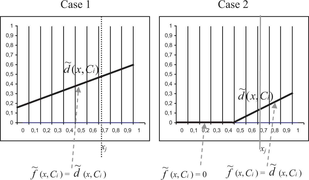
Virtual opportunity distributions.
For each 2 × 2 contingency table showing the relationship between access to G and membership of a social subgroup Ci
, there exists a virtual joint density
Define mi
the fraction of the whole population which belongs to Ci
and ri
the rate of access to G of members of Ci
.
The family of joint densities
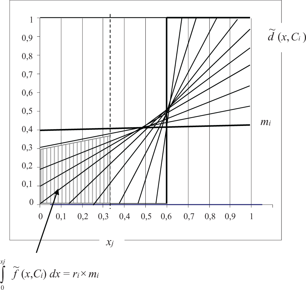
Family of virtual joint densities
Properties of the
coefficients
As showed in Bulle (2009:3.2), several general properties of the
We have
When there is no distinction in terms of relative opportunity of access to G between Ci
and the whole population, the representative curve of
The surface xj
× mi
is represented by the square at the bottom left of Figure 2. It is then obvious that:
The
Insensitivity to xj
variations stems from the definition of
Several specific properties of the
If subgroups are aggregated,
If
Interpretation of
as an overall measure of inequality within the selection process
According to the Theoretical assumptions and Properties of the The coefficient The coefficient
Calculation of
Table 4 shows the relationship between access to G and membership of
Parameters of the 2 × 2 Contingency Table (I).
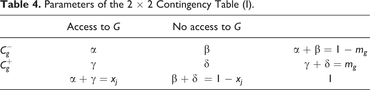
According to our assumptions,
Define the straight line
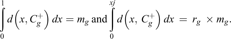
It can easily be shown that
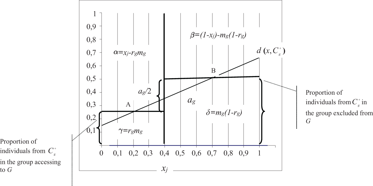
Graphic representation of the contingency table data presented on Table 4 and regression line
From the definition of
From these equations, we can also deduce that
This gives us the two cases presented in the Theoretical assumptions subsection. Condition (I) is fulfilled: Then—and essentially whenever the general case applies— In other cases, condition (I) is not fulfilled. The function
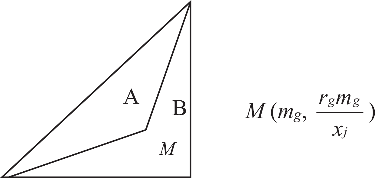
Figure 4 illustrates case (2) when
A specific case.
Define xk
as the abscissa of the intersection between
When
Finally, even if, in the general case—condition (I) fulfilled—the inequality index
The selection process results, inequality within the selection process, and the issue of linearity
It should be noted that the assumption of linearity that underlies the measurement of the inequality within the selection process
For example, if G represented a certain salary level S, and inequality between men and women was the subject of the analysis, the ranking of the population in terms of salaries would not be useful for determining inequality of opportunity within the selection process for access to the defined salary level S. The study of access to salary level S would just lead to the application of a cutting point in this ranking. By regularly spreading the discrepancies in the selection process results across the continuous distribution of relative opportunity of access to this salary level S, linearity allows us to compare the unequal outcomes of the selection process between populations or across time.
Now, if G was a continuous good, the comparison of inequality within the selection process between populations, or between periods of time, would require to compare inequality within the selection process for access to the various percentile groups at stake. Alternatively, let us suppose that there is a hierarchical ranking of n discrete goods Gk (constituting a vertical ordering of, for instance, education levels), such that all individuals accessing any higher ranked good Gk + 1 would have access to the lower ranked good Gk . We would dispose in such a case of n overall measures of inequality in the selection process for access to the n goods Gk . We can consider that these n ranked goods, from the less selective to the most selective good, Gk , are cutting points within the distribution of relative opportunity of access to a continuous good G (if the goods Gk are levels of education, then G represents the “formal education” good). These various cutting points may suffice to assess, by linear extrapolations for instance, inequality within the selection process for access to each specific percentile group (Bulle 2009:581).
Let us take the example of a specific case to illustrate the role of the assumption of linearity. We assume we have a selection process for access to a discrete good G based on a specific rule of selection such that the equation of the curve representing the (real) joint density function
Note that if we calculate the values of the various odds ratios in order to compare relative opportunity of access to G between these same contexts, we find successively 195.2, 51.5, 27.9, 19.3, 15.4, 13.9, 13.9, 16.0, and 25.2. Relative opportunity of access to G, as measured by the odds ratio, decreases rapidly from an opening up of G of 10% to an opening up of 60% and then increases somewhat to an opening up of 90%. The diagnostic of the evolution of opportunity is thus quite different from that offered by the measure of inequality within the selection process, and such a difference does express the various aspects of inequality these indexes capture, that is, one compares the outcomes of the micro-social processes that generate unequal access to G across contexts, irrespective of the opening up of access to G, and the other one compares a degree of intrinsic association between access to G and social stratification.
Comparison of the
Index With Classical Inequality of Opportunity Measures
In the following, we suppose that
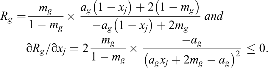
Relationship With the Ratio of Proportions
The access rate for members of
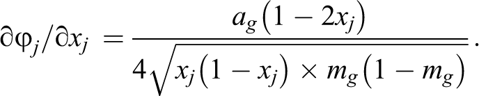
The derivative of
Define
Note that Rg
is not margin insensitive. For instance, if xj
, the fraction of the population gaining access to G, increases, giving
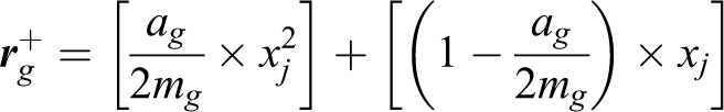
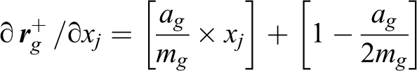
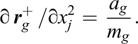
Substituting α with x − γ and γ with (½ ag × xj 2) + (mg − ½ ag ) xj (see Tables 4 and 5) in the formulae for Rg mentioned previously, simplifying by x (which is not null) and factorizing, we obtain:
Parameters of the 2 × 2 Contingency Table (II).
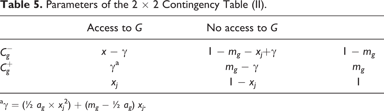
aγ = (½ ag × xj 2) + (mg − ½ ag ) xj .
Define the ratio of exclusion rates:
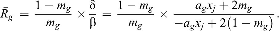
Like Rg
,
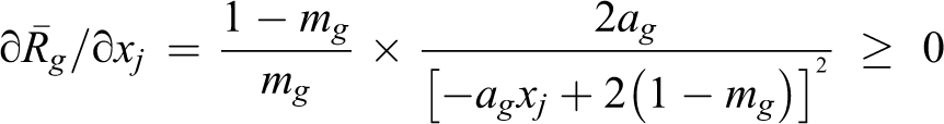
Relative risk of exclusion from G for members of
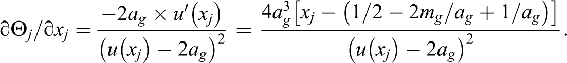
Relationship With the Odds Ratio
The odds ratio Θ
j
compares relative chance of access to G and relative risk of exclusion from G for members of
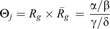
We obtain
Θ
j
can be written
With
Note that, according to the conditions met by the parameters, it can be shown that Θ j varies positively with ag .
That is,
If,
If 0 < A < 1, (xj
– A) ≥ 0
and increases until xj = 1.
Note that if mg
= ½ the curve
If
Relationship With the Difference in Access Rates
The difference in access rates, Dg is calculated by subtracting the proportion of the disadvantaged subgroup which is selected from the proportion of the advantaged subgroup which is selected.
Dg
can reach its maximum of 1 only if the proportion of members of
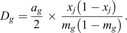
Inequality Dg increases linearly with ag .
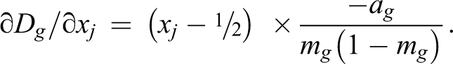
The difference in access rates increases until xj = ½ and then decreases. Dg tends toward 0 when xj tends toward 0 or toward 1, that is, when access to G is either rare or widespread. The axis of symmetry xj = ½, with regard to variations of Dg , is explained by the symmetry of the parts played by the selected and the nonselected individuals.
Relationship With the Phi Coefficient of Association
N indicates the size of the population.
In the case of a 2 × 2 table, the phi coefficient can be considered as a coefficient of linear correlation between two binary variables.
Define σ
g
and σ
j
as the standard deviations of the two variables (membership of
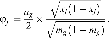
Inequality φ j increases linearly with ag .
φ j increases with diffusion of G until xj = ½ and then decreases. φ j tends toward 0 when xj tends toward 0 or when xj tends toward 1. As it is the case for Dg , the axis of symmetry xj = ½, with respect to variations of φ j , is explained by the symmetry of the part played by the selected and the nonselected individuals.
Relationship With the Gini Coefficient
The Gini coefficient, Gj
, measures the concentration of access to G in the present framework. It represents a ratio of areas on the Lorenz concentration curve diagram (
Lorenz concentration curve.
We find
Thus, we have
Inequality Gj increases linearly with ag .
The Gini coefficient, Gj , decreases linearly with diffusion of G across the population, with a speed proportional to ag . From this concentration defined by individuals gaining access to G, the concentration defined by individuals who fail to gain access to G can be deduced:

These two concentrations vary in opposite directions when diffusion of G increases. The expression of these two concentrations with respect to coefficient
Relationship with the Marginal Matching Coefficient
Blackburn and Marsh (1991), and Blackburn et al. (1995) proposed a measure—the marginal matching coefficient MM—to address the problem of sensitivity to marginal variations in segregation analysis. MM requires one to provide matched distributions in the two margins of the basic segregation table, that is, to change the definition of advantaged versus disadvantaged units or, as here, social subgroups and define two sets of units such that their distribution in each period is identical to the distribution of the segregation criteria (fractions of men and women in the labor force for instance; or as here, fraction of individuals gaining access to G) such that it is possible in principle for every member of the advantaged subgroups, and none of the members of the other subgroups, to meet the criteria for selection. This calculation is done by ranking the units (social subgroups in the present example) according to the fraction without access to G—this ranking may be carried out finely using an index based on a continuous scale of social advantage—and then by calculating the cumulative fraction of the population starting at the top of this ranking, and moving along the cumulative distribution of the social subgroups, until it equals 1 − xj
(the proportion of the population excluded from G). This procedure “matches” marginal totals 1 − xj
and xj
to the respective proportions of disadvantaged and advantaged subgroups m
MM and 1 − m
MM in the population. Therefore, the disadvantaged group
On the basis of this segregation table with matched margins, several statistics of association coincide with MM, in particular, the difference in access rates, the difference in proportions when comparing contingency table columns, and the phi coefficient:
Therefore, as in the general case (I), we have
Index Variations With G Diffusion, Some Illustrations
Figures 6 to 8 illustrate the variation of the classical indices listed previously with respect to diffusion of G (from xj
= 10% to xj
= 90%) when the degree of inequality within the selection process
As defined, Dg
and φ
j
are positive and thus range from 0 to 1, which is the variation interval of Gj
, with 0 indicating no relationship. To make comparisons of how these indices vary with diffusion of G easier, the variation intervals of indices Rg,
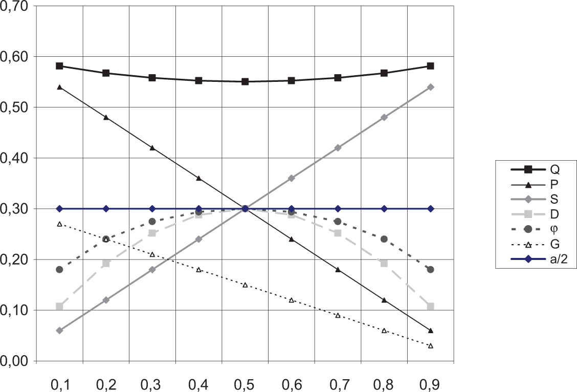
Variation of inequality indices with respect to G’s diffusion–mi = 0.5 and ai = 0.6.
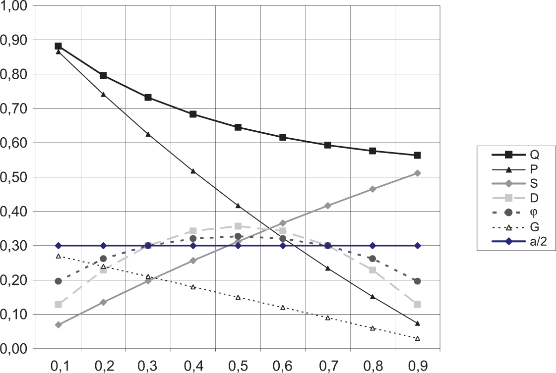
Variation of inequality indices with respect to G’s diffusion–mi = 0.3 and ai = 0.6.
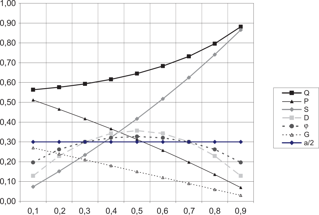
Variation of inequality indices with respect to G’s diffusion–mi = 0.7 and ai = 0.6.
Measuring Inequality Within the Selection Process: Return to the 1944 Act Example
We now have available all the instruments and data required to assess the evolution of inequality within the selection process for access to lengthy secondary education for English children born in the first half of the twentieth century. To begin with, we look at the results obtained from data studied by Little and Westergaard. We have supplemented the data provided in their tables with data from Floud (1954) and the Crowther Report (1959). Our discussion focuses on boys in order to be able to extend this study with an analysis of data published by Halsey et al. (1980) and also used by Blackburn and Marsh (1991).
We have seen that Little and Westergaard’s account of inequalities in access to selective secondary education was mixed, depending on whether it was based on the evolution of chance of access or risk of exclusion. The odds ratio, which takes both into account, compares the chances of children of parents belonging to the more advantaged categories—Professionals and Managers—with the chances of children of parents belonging to the less advantaged categories—Semiskilled and Unskilled Manual Workers—and has a value of 58 for the cohort born before 1910, 22, 15, and 16, respectively, for the three following cohorts (data from Table 1). Based on this index, one might conclude that initially there was a significant decrease in inequality of opportunity, with no reduction over the last two cohorts. When the same statistic, the odds ratio, is calculated for boys only (data from Table 6), the decrease in inequality is less pronounced, with a slight strengthening over the last two cohorts the—values for successive cohorts are 25, 18, 13, and 16, respectively. However, if inequality within the selection process is measured by
Proportions of Boys in Different Classes Obtaining Education of a Grammar School Type,a by Birth Cohort.
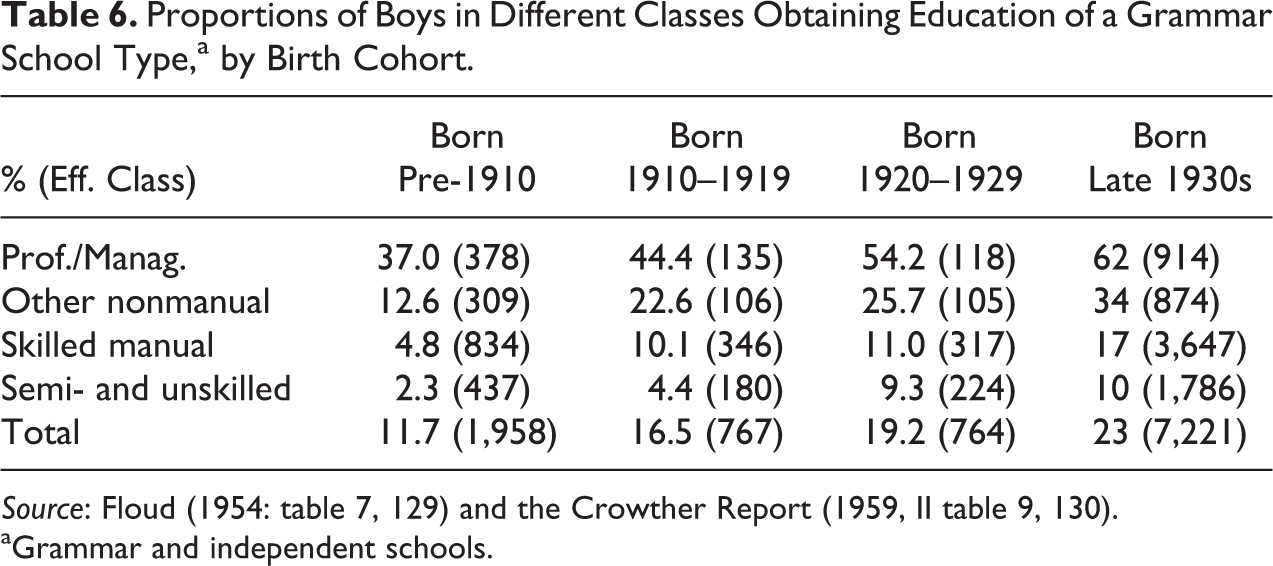
Source: Floud (1954: table 7, 129) and the Crowther Report (1959, II table 9, 130).
aGrammar and independent schools.
Inequality in the Selection Processa
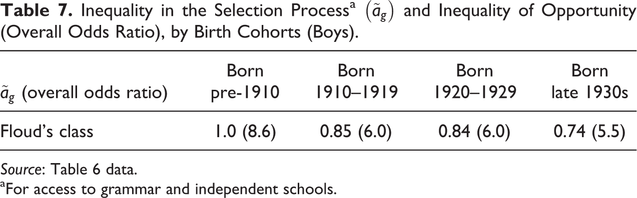
Source: Table 6 data.
aFor access to grammar and independent schools.
While the odds ratio allows for the removal of ambiguities arising from conflicting accounts of the evolution of chance of access and risk of exclusion, knowing inequality within the selection process allows us to distinguish between changes that are attributable to unequal outcomes of micro-social processes and changes attributable to margins variation. Thus, we can see that inequality within the selection process decreases over the sample period, especially for boys reaching 11 years in the 1920s and at the end of the 1940s. In other words, the situation described by Little and Westergaard (1964:312-13) where “the overall expansion of educational facilities has been of greater significance than any redistribution of opportunities,” with inequalities probably “shifted to later stages of education where selection would then operate”—that is, a situation that can be understood as unchanged regarding inequality within the selection process—may be discussed somewhat.
We will now compare the results of different analyses of Halsey et al.’s data. Based on the MM calculation, Blackburn and Marsh observed a growing trend of inequality before 1944, which was initially reversed by the Act but then inequality rose again to a higher level than before the Act: The relative shortage of selective places for the last cohort studied, as a result of the “baby boom,” they suggested, resulted in greater competition and a reinforcement of the “effective value of social advantage” (Blackburn and Marsh 1991:529). Based on their class categorization, the overall odds ratio indicates a similar pattern of inequality; we can see that this is due to a trend in the inequality within the selection process
Inequality in the Selection Process (
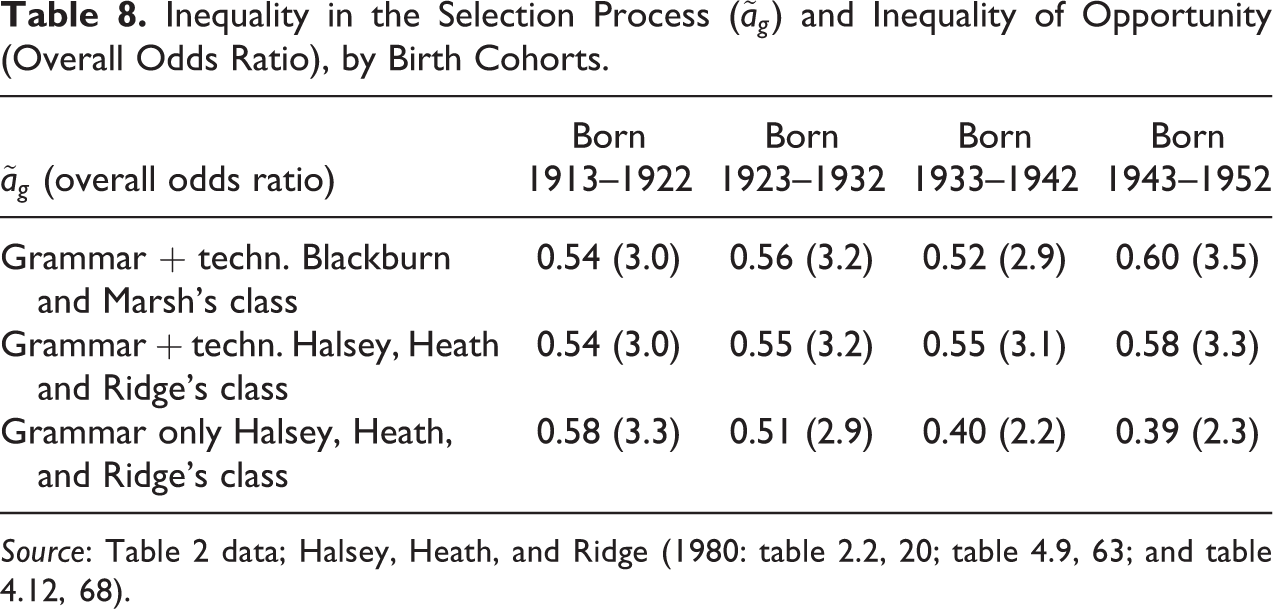
Source: Table 2 data; Halsey, Heath, and Ridge (1980: table 2.2, 20; table 4.9, 63; and table 4.12, 68).
We note that the significant differences in the values of the various indices depend on whether they are based on Floud’s classification and data (seven categories) or on Little and Westergaard’s grouped classification (three classes) or else, on Halsey et al.’s own classification and data (three classes). 12 Floud’s more detailed classification allowed us to distinguish more precisely the advantaged (access rate above average) from the disadvantaged groups (access rate below average), than with Halsey et al.’s classification. Consequently, we will only be able to compare trends in inequality of opportunity, not the extent of inequality, across measures.
The first three cohorts in Halsey et al.’s analysis can be compared to the last three cohorts in Little and Westergaard’s analysis, notwithstanding the 3-year difference in dates of birth. However, the comparison with previous analyses of Little and Westergaard’s data reveals differences in trends. We observed decreasing inequality within the selection process following the Act, while the situation seems to get worse, after a long, stable period, when we look at results we obtain with Halsey et al.’s data. But, these authors noted an important difference is that they included technical schools in their group of selective schools and Little and Westergaard did not.
Significant differences in trends are revealed when we consider grammar schools only. Inequality within the selection process
These patterns of change in inequality within the selection process can be compared with those observed when we include technical schools in the analysis. The difference in the evolution observed is due to the change in opportunity within the selection process for access to technical schools—variations in the availability of places having, as we know, no direct effect on these changes: 14 increasing inequality in the 1930s and 1940s with a slowing of the upward trend at the end of the 1950s. We suggest that this growing trend of inequality within the selection process for access to technical schools is also an effect of the reduction in differences between social groups regarding their choices of schooling during this period.
The global trends with respect to inequality within the selection process are slightly to the benefit of advantaged social categories when all types of selective schools are considered, but it should still be noted that disadvantaged social categories benefited from a reduction in inequality within the selection process for access to the most selective schools, that is, grammar schools.
To summarize, by separating the effects of inequality within the selection process from the effects of the margins, we obtain a better understanding of the social processes at work. By referring to the evolution of inequality within the selection process, we hypothesize that the development of less socially differentiated attitudes to education from the beginning of the twentieth century—that is, the increased investment by disadvantaged categories in lengthy studies and conversely, the increased investment by advantaged categories in technical studies—underpin two opposing long-term trends that are independent of both the changing number of places in selective schools and the 1944 Act; one is an increase in the inequality within the selection process for access to technical schools and the other is a decrease in the inequality within the selection process for access to a grammar school education, with a trend to stabilization in the last period.
Conclusion
For the purpose of distinguishing the effects of the margins from those of the unequal outcomes of micro-social processes, with respect to inequality of access to a discrete good G, the index of inequality within the selection process
This index offers a solution to an important class of problem in sociology: explanatory accounts of inequality of access to a discrete good G across populations or across time. Such problems have been the objects of regrettably sporadic debate over the last quarter of century. Argument has centered on the issues of margin insensitivity and allocation mechanisms. The aspect of inequality captured by the
Our analysis of the changes in classical measures of inequality with diffusion of G, while inequality within the selection process
Footnotes
Appendix
Acknowledgements
The author would especially like to thank two anonymous referees of SMR for their very constructive comments and suggestions on an earlier version of this paper.
Declaration of Conflicting Interests
The author(s) declared no potential conflicts of interest with respect to the research, authorship, and/or publication of this article.
Funding
The author(s) received no financial support for the research, authorship, and/or publication of this article.