Sage Journals: Discover world-class research

Abstract

World Tourism Organization (UNWTO) is the major source of internationally comparable data on tourism. However, UNWTO data has two drawbacks: it focuses on international trips and ignores differences between regions within individual countries. Alternative sources of big data are increasingly used to enhance tourism statistics. In this paper, we combine traditional information sources with gridded population dataset and Airbnb data to address the limitations of UNWTO statistics. We produce a map of world tourism destinations measured by the number of tourism visits and tourism expenditure in 2019, before the COVID-19 pandemic. We then identify hot spots of tourism and compare the level of spatial concentration of tourism to that of global population and economy. The results illustrate how supply and demand shape the global distribution of tourism, highlight the dominance of domestic travels in global tourism mobility and may help planning tourism policy in the face of current global challenges.

Keywords

international tourism domestic tourism geography big data dasymetric mapping Airbnb

Introduction

Tourism mobility and the tourism industry are geographically uneven phenomena. The spatial distribution of tourism flows and their economic effects have long been among the interests of tourism geographers (Lew, Hall, and Timothy 2008; Pearce 1995). The most important source of quantitative data on the numbers and economic effects of tourism in different parts of the world is the World Tourism Organization (UNWTO). However, UNWTO data on tourism trips has two major drawbacks. First, while comprehensive in terms of international flows, it is incomplete and patchy in describing domestic travels, which represent the majority of global tourism mobility (Bigano et al. 2007; UNWTO 2020a). Second, UNWTO data treat entire countries as tourism destinations, while the distribution of tourism visits is not uniform within individual countries: usually, tourists visit some cities and regions more frequently than others. Many countries gather and publish tourism statistics on lower territorial levels, but statistical methodologies are incoherent in terms of the territorial divisions, definitions, and methods of collecting data. Hence, it is difficult to combine data from national sources to produce a globally comparable dataset.

In this paper, we attempt to combine traditional information sources (UNWTO and national statistics) with alternative sources of large-volume geo-referenced data (gridded population dataset Global Human Settlement Population Layer (GHS-POP) 2015, and geo-referenced data on Airbnb offers in 2019) to produce a detailed and globally comparable map of tourism destinations measured by the number of tourism visits and the amount of tourism expenditure. Based on the result, we identify major global tourism hotspots, and measure the level of spatial concentration of tourism visits and expenditure worldwide in relation to global population and economy. The findings provide insight into the territorial differences in the magnitude of social, environmental, and economic impacts of tourism. They may also help to better understand the geographic dimension of the current challenges that tourism faces, including recovery after the COVID-19 pandemic (Zenker and Kock 2020) and mitigation of, and adaptation to, climate change (Scott, Hall, and Gössling 2012).

Before presenting the detailed methods and results of the analysis, we discuss the existing literature on the determinants and patterns of tourism flows, and review the recent applications of geo-referenced data to enhance tourism statistics. The paper is concluded with a discussion of the results, in terms of the implications for tourism geography and tourism management practices. In the Appendices and Supplemental Files, we provide detailed results of the analysis for further re-use.

Literature Review

Patterns of Tourism Flows and Distribution of Tourism Destinations

Tourism destinations are not evenly distributed across the world. Some countries, regions, and cities are visited more often than others. The first explanation for this is the uneven distribution of tourism resources that attract visitors (Lew 1987; Warszyńska and Jackowski 1978). Destinations for leisure tourism are often located near seacoasts in favorable climatic conditions (Gómez Martín 2005), and specific natural conditions are required to participate in active forms of tourism such as ski tourism (Hinch and Higham 2011). Sightseeing tourism concentrates in locations of high value for cultural and natural heritage, including those recognized by United Nations Educational, Scientific and Cultural Organization (UNESCO) as World Heritage Sites (Yang, Lin, and Han 2010). Yet, the simple existence of physical and cultural resources must be supplemented by the development of tourism industry: infrastructure that creates industrialized attractions, accommodation, transportation, and other services (Leiper 1979; Smith 1994).

Looking at the destination perspective alone is not sufficient to understand the geography of tourism flows. One should consider the relations between tourism origins and destinations, and the transit routes (Leiper 1979). A core–periphery model proposed by Christaller (1964) expects tourism to disperse over the peripheries, following a different pattern than other economic activities, which tend to group together in central places. A core–periphery relation could be noticed in international tourism statistics in history, when European and American countries were clearly divided into central economies representing tourism origins (e.g., United States of America, West Germany) and internal peripheries serving as tourism destinations (e.g., Spain and Portugal; Williams and Zelinsky 1970). On the lower territorial scale, the central areas creating tourism demand are mainly cities. The geographic scope of travels is limited by time and cost of transport, hence distance decay (McKercher, Chan, and Lam 2008) explains the formation of urban recreational hinterlands (Greer and Wall 1979). The distance of travels depends on their purpose, length, and recurrence, so to understand the distance decay it is important to consider a wide spectrum of human mobility (Hall 2005).

The core–periphery pattern is no longer sufficient to describe the contemporary geography of tourism flows. Cities are no longer mere generators of tourism trips, but increasingly also tourism destinations. Cities attract visitors with historic sites, congresses and business meetings, cultural and sport events, and shopping opportunities (Law 1993). In recent decades, attracting tourists was treated by urban governments and stakeholders as part of the strategy in global competition between cities (Abrahamson 2004). In Europe, before the pandemic urban tourism grew faster than tourism in non-urban areas, and the growth of urban tourism was accompanied by increasing concerns of overtourism (Milano 2017; Nilsson 2020).

Tourism mobility patterns are not constant over time. The evolution of tourism destinations follows various paths and stages from exploration to decline, as described by the Tourism Area Life Cycle model (Butler 1980) or evolutionary approaches to tourism geography (Brouder et al. 2017). Tourism geographers have recently been less engaged in identifying and measuring tourism flows, focusing instead on tourism impacts and tourists’ experiences (Hall and Page 2014; Williams 2009). Yet, understanding spatial patterns of tourism is still relevant not only due to ongoing transformations of tourism demand and destinations following global socio-economic processes, but also because of the need to mitigate and adapt to climate change (Peeters and Landré 2011; Scott, Hall, and Gössling 2012). The current study joins the developing line of research utilizing big-data sources (Bauder 2019; Li et al. 2018) to understand the spatial patterns of tourism on spatial and temporal scales more detailed than those offered by conventional statistics.

New Methodological Approaches to the Statistical Mapping of Tourism Destinations

Presenting and explaining the patterns of international tourism flows faces problems of availability of statistical data and its comparability across countries. The World Tourism Organization (UNWTO) has popularized a standard definition of international tourism trips and collects globally comparable data on international tourism arrivals for most countries of the world. This data has its limitations, however. Apart from imperfect comparability of data from various countries and missing data, two basic problems arise. First, data on domestic tourism, the majority of global tourism mobility, is only fragmentary. Second, statistics usually apply to entire countries, so variations within individual countries are not presented.

As an effect, an interpretation of UNWTO data may be biased by the configuration of political borders. The high number of tourists visiting European countries (half of international tourist arrivals; UNWTO 2021a) is partially a result of the political fragmentation of this part of the world. For example, if the state of Florida was treated as a separate country, then, with the estimated number of yearly arrivals exceeding 100 million (Visit Florida 2019), it could surpass France as the largest tourism destination. Also, the statistics of international mobility in East Asia are influenced by the fact that all travels between China and the Special Administrative Units of Hong Kong and Macau are considered international trips (Pratt and Tolkach 2018). If they were treated as domestic instead, the numbers of international tourists’ arrivals to Hong Kong would decrease by 69.5%, and to Macau by 89.5% (UNWTO 2020b).

Some efforts were made to address these issues. Bigano et al. (2007) created a database of domestic and international tourism arrivals in administrative regions based on national statistical sources from 1995. Peeters and Landré (2011) estimated the numbers of domestic tourism to measure global length of tourist travels. Mastercard (2019) and Euromonitor (Yasmeen 2019) publish yearly reports on arrivals and expenditures of international tourists in major global tourism cities, based on official statistics and their own estimations. A consortium of Austrian academic, statistical and tourism marketing organizations maintains TourMIS database on European countries, selected cities and attractions (TourMIS 2021; Wöber 2003). It is based on official statistical sources coupled with the data supplied by tourism professionals from all over Europe, which makes it the most comprehensive database on European city tourism, but also limits the scope and comparability of data.

In recent years, new opportunities for measuring tourism flows with high spatial and temporal resolution are provided by employing user-generated big data (Eurostat 2017; Li et al. 2018). Previous studies have proven it is useful to acquire information about tourism distribution from mobile tracking techniques (Deville et al. 2014; Saluveer et al. 2020), geo-located tweets (Hawelka et al. 2014) and photographs (Preis, Botta, and Moat 2019; Wood et al. 2013), travel reviews (Tilly, Fischbach, and Schoder 2015), website traffic indicators (Gunter and Önder 2016), social media activity (Chen, Becken, and Stantic 2021; Önder, Gunter, and Gindl 2019), or web travel diaries (Zeng 2018). Vaguet and Cebeillac (2021) proved that Airbnb data can be used to infer about spatial and temporal characteristics of tourist trips taking visitors to Iceland as a sample.

So far, the only example of the use of big data to improve the detail of tourism distribution statistics of a large area was made by Batista e Silva et al. (2018). The authors integrated traditional statistics with the location of accommodation establishments derived from Booking.com and TripAdvisor platforms to create a database of tourism in 100 × 100-m grid cells in four seasons of the year. Methodically, Batista e Silva et al. (2018) study drew from the idea of dasymetric mapping, which integrates statistical data with ancillary (e.g., land-use) data to show more accurate distribution of population (Leyk et al. 2019; Semenov-Tian-Shansky 1928). The dasymetric method was used in classical form to map tourism at smaller spatial scales (Vaz and Campos 2013). The geographic database elaborated by Batista e Silva et al. (2018) is similar to multiple grid population databases (Leyk et al. 2019) and grid GDP database by Kummu, Taka, and Guillaume (2018). This approach is reliant on statistics that are available from Eurostat, so it cannot be replicated for other areas than Europe. Our study, in turn, has a global scope and the results enable comparisons across different parts of the world.

Research Procedure, Data, and Methods

We followed a three-step research procedure outlined in Figure 1. First, based on official statistical sources, we collected data on the numbers of international tourism arrivals, domestic tourism trips, and tourism expenditure in countries and administrative units of large countries. At this stage we also estimated missing data where necessary. Second, we disaggregated the numbers of tourists (international tourist arrivals and domestic tourism trips) in each country and administrative unit into hexagonal grid cells using statistical dasymetric modeling with area, population, and locations of Airbnb offers used as ancillary variables. To estimate the functions linking these variables with the number of tourist visits we used Eurostat (2020a) data on the numbers of tourists visiting second level regions according to the Nomenclature of Territorial Units for Statistics (NUTS-2 units) in the European Economic Area. After estimating numbers of domestic and international tourists visiting each grid cell, we calculated the estimated local expenditures of international and domestic tourists, and ratios of tourism visits per inhabitant and tourist expenditures per Gross Domestic Product (GDP). Third, we found the global hotspots of the largest concentration and intensity of tourism visits and expenditures, and we calculated the concentration index of tourism visits to compare it with the territorial concentration of global population and GDP. The analysis was done in R, and cartographic presentation in ArcGIS. We presented results on maps and appended datasets. Apart from that, we append the R file and raw data files produced at consecutive steps of the analysis, which enables the readers to reproduce the analysis. Below, we describe in detail each stage of the procedure.

Figure 1.

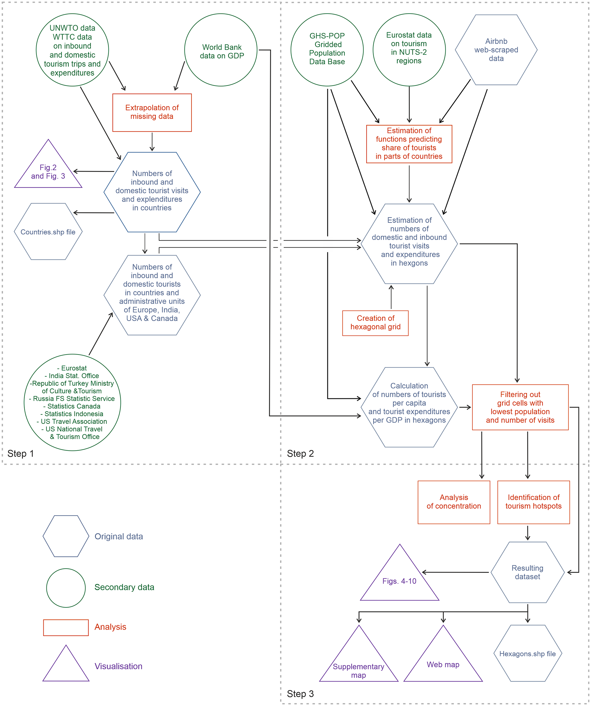
Research procedure.

Collecting and Complementing Official Statistics on Tourism in Countries and Sub-National Territorial Units

The first step of the analysis comprised the collection of data on numbers of inbound tourism arrivals and domestic tourism trips and tourism expenditure by country and territory provided by World Tourism Organization (UNWTO) and World Travel & Tourism Council (WTTC) statistics (UNWTO 2020b; World Bank 2020). We then estimated missing values in the dataset. Later, where possible, we disaggregated the data into smaller territorial divisions of large countries (Figure 1).

Statistics on countries and dependent territories

The UNWTO statistical database includes data on inbound tourism arrivals and domestic tourism trips in 222 countries and dependent territories of the world (UNWTO 2020b). Data is based on information from national statistical institutions. Some countries have not yet delivered data for the year 2019. In such situations, we used the last available data, extrapolating them proportionally to average global growth. We used data on total inbound arrivals, including same-day visits, for countries that do not separately report the numbers of tourist arrivals. They are mostly island countries with a naturally limited number of international same-day visits. At this stage, we excluded from the analysis countries and territories for which UNWTO did not provide data on inbound arrivals or for which data estimation was impossible due to missing socio-economic data in the World Bank (2020) database. As a result, 195 countries and territories were used in further analysis.

Of those 195, only 75 had data on domestic trips available (including data extrapolated from earlier years in cases where data for 2019 was missing). We estimated these missing data based on linear regression models, similarly as Bigano et al. (2007) and Peeters and Landré (2011) did. As explaining variables, we used socio-economic indicators according to the World Bank (2020). Where necessary, previous figures were extrapolated to 2019 based on data on previous years and the global trend. We filled missing numbers in the database using The National Institute of Statistics and Economic Studies (INSEE, 2019) statistics on the populations of French overseas departments and figures for Cuba and Taiwan compiled from the Central Intelligence Agency, International Monetary Fund (IMF) and United Nations databases. We assumed that the number of domestic trips per capita is affected by the level of socio-economic development of the country, the availability of domestic destinations measured by country area, and differences between global regions. We tried various constructions of the model to obtain the best fit with all predictors (including any region as a categorical value) significant at p < .05. The final equation is as follows (see Appendix A for detailed estimation of the regression model parameters):

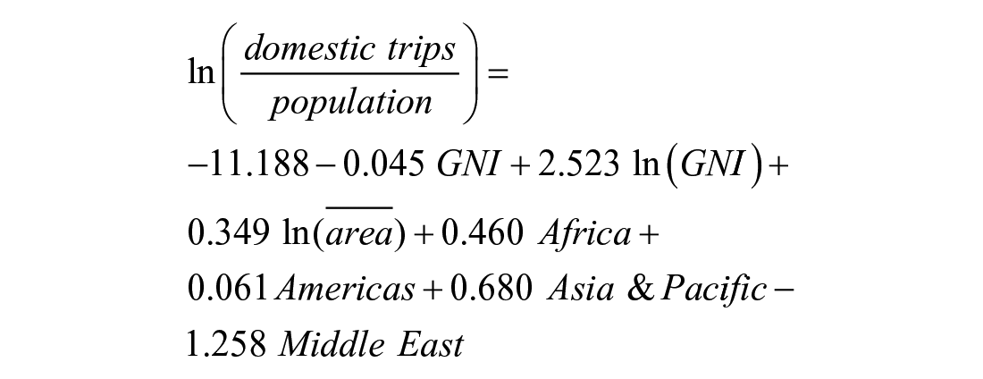
\begin{array}{l} \ln (\frac{d o m e s t i c t r i p s}{p o p u l a t i o n}) = \\ - 11.188 - 0.045 G N I + 2.523 \ln (G N I) + \\ 0.349 \ln (\bar{a r e a}) + 0.460 A f r i c a + \\ 0.061 A m e r i c a s + 0.680 A s i a & P a c i f i c - \\ 1.258 M i d d l e E a s t \end{array}

Tourist activity is highly dependent on the level of economic development measured by gross national income per capita in purchasing power parity (GNI). Its impact on tourism travels is non-linear, so we included both raw values and their natural logarithm as predictors. We assumed the area of a country would raise the number of residents’ domestic trips (by increasing choice of domestic destinations), but this effect would be limited in the case of big countries. So the $\bar{a r e a}$ variable takes values (in km²):

\bar{a r e a} = {\begin{matrix} a r e a, i f a r e a < 500, 000 \\ 500, 000, i f a r e a \geq 500, 000 \end{matrix}

There are also important differences between countries in various regions of the world. Hence, we included dummy variables denoting location in various part of the world according to the UNWTO division, with Europe as a reference region.

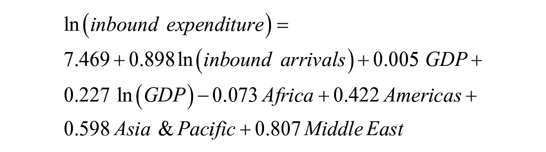
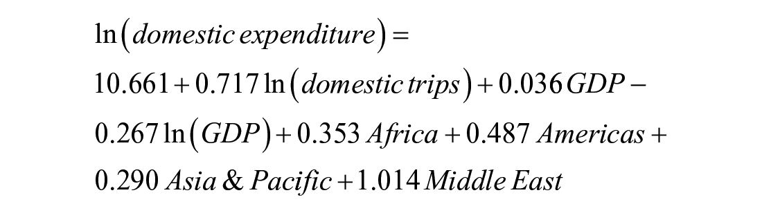
Data on inbound and domestic tourism expenditure is derived from the World Travel and Tourism Council and we accessed them via the World Bank (2020) database. Twenty-three and twenty-one countries and territories had missing data on inbound and domestic tourism expenditure, respectively. We estimated these values using the numbers of inbound arrivals/domestic trips and nominal GDP per capita in current USD as predictors. The equations are as follows (see Appendix A for detailed estimation of the regression models parameters):

\begin{array}{l} \ln (i n b o u n d e x p e n d i t u r e) = \\ 7.469 + 0.898 \ln (i n b o u n d a r r i v a l s) + 0.005 G D P + \\ 0.227 \ln (G D P) - 0.073 A f r i c a + 0.422 A m e r i c a s + \\ 0.598 A s i a & P a c i f i c + 0.807 M i d d l e E a s t \end{array}

\begin{array}{l} \ln (d o m e s t i c e x p e n d i t u r e) = \\ 10.661 + 0.717 \ln (d o m e s t i c t r i p s) + 0.036 G D P - \\ 0.267 \ln (G D P) + 0.353 A f r i c a + 0.487 A m e r i c a s + \\ 0.290 A s i a & P a c i f i c + 1.014 M i d d l e E a s t \end{array}

The resulting data on countries is available in the countries.shp file in the Supplemental Files.

Disaggregating data into administrative regions of selected countries

To enhance the spatial resolution of the dataset, we divided some countries into smaller territorial units and calculated tourist visits and expenditure in each unit based on national statistical sources. We performed this operation only for countries with relatively large areas, large numbers of tourists, and the availability of appropriate data.

In the case of EU countries, the United Kingdom, Norway, and Switzerland, we used Eurostat (2020a) data on the number of international and domestic tourism arrivals in NUTS-2 territorial units in 2019 to refine the previously obtained data on countries. We did not directly use Eurostat data for the entire countries, as for some countries they differ from those provided by UNWTO, due to methodological differences. Instead, we used Eurostat data to proportionally divide the numbers of international arrivals, domestic trips and, similarly, tourism expenditure into territorial units of countries.

In the case of Canada we followed a similar procedure, assuming that the 2019 distribution of total tourism arrivals and expenditures in 13 provinces and territories was proportional to the distribution of tourism demand in 2014, while the distribution of international tourism arrivals and expenditures was proportional to international exports from tourism in 2014 (Statistics Canada 2018). In India we divided the numbers of tourism visits and expenditure across states and union territories proportionally to the distribution of inbound tourism arrivals and domestic tourism trips in 2017 according to the Indian Statistical Office (Government of India 2018). In the case of Indonesia, the basis for the division of national numbers into provinces was the distribution of international and domestic guests in both classified and non-classified hotels in 2018 (Statistics Indonesia 2020). In Turkey, we assumed that the distribution of international and domestic tourism visits and expenditure in provinces in 2019 was proportional to the distribution of international and domestic tourism guests in tourism establishments in 2016 based on the last available data published by the Republic of Turkey Ministry of Culture and Tourism (2017a, 2017b).

In the case of Russia we based the disaggregation on the statistics on foreign citizens and Russian citizens accommodated in collective accommodation facilities (Federal State Statistic Service 2021a, 2021b). Note that, for data consistency, we use Russian statistics on Republic of Crimea and Sevastopol, despite their disputed political status, as Ukrainian tourism statistics do not provide information about the region (Ukrstat 2019). Still, this data should be treated with caution (StopFake 2018).

A more refined calculation was performed in the case of the United States of America, based on several statistical sources. We assumed that the distribution of total tourism visits and expenditures across 50 states and the District of Columbia was proportional to the mean of the share of total tourism expenditures and of the total employment in tourism in 2018 according to the U.S. Travel Association (2020). The distribution of inbound tourism arrivals was calculated based on data of the National Travel and Tourism Office (2020), by adding together separately calculated overseas arrivals, arrivals from Canada, and arrivals from Mexico, which in turn was aggregated from air trips and arrivals by ground means of transportation estimated based on the distribution of population of Mexican origin, assuming a large proportion of visiting friends and relatives (VFR) tourism. Later, total tourism expenditure was divided into inbound and domestic tourism based on the proportions between domestic and international visits in states.

The detailed source data for state disaggregation is collected in the states.xlsx file in the data collection. The final data for sub-national units are provided in the states_nuts.shp file.

Disaggregating Tourism Numbers Into Grid Cells

The next step of analysis was to disaggregate the numbers of tourists and tourism expenditures into territorial units smaller than the countries or administrative regions (Figure 1). We used the term total tourist visits to denote the sum of the unit’s share in total international tourist arrivals and its share in the endpoints of domestic tourist trips. Due to differences in administrative divisions of countries around the world, we used geometric grid cells as the units of analysis. We cannot assume that tourist numbers are uniformly distributed over the territories of the countries and regions. Therefore, we followed a dasymetric mapping using statistically derived weights informed by multiple ancillary variables (Leyk et al. 2019): area, population, and the number of Airbnb reviews.

The assumption that the distribution of tourism is somehow proportional to the area of territorial units is justified by Christaller’s (1964) model of tourism location. Yet, hosting tourists requires infrastructure and usually happens in populated places, so we used population as a second ancillary variable. However, these two variables do not suffice to notice variability in tourism location caused by the distribution of natural conditions, attractions, amenities, accessibility, etc. Following the approach of Batista e Silva et al. (2018), we assumed that the supply of accommodation offered on global internet platforms can serve as a proxy of the distribution of tourism visits. We used the Airbnb platform due to its global presence. Airbnb, established in 2008, is now the largest peer-to-peer rental platform in the world (Dolnicar 2018), marketing more than seven million rental homes, apartments, rooms, and other forms of accommodation (Airbnb 2020). Even though the original idea of the company was to sell unused space in one’s own dwelling in periods of high demand for accommodation, it now serves mostly for commercial rental of tourism accommodation (Adamiak 2019), so we can expect the distribution of the offer to be representative for other forms of tourism accommodation. The general correlation between Airbnb presence and other tourism accommodation and tourism activity has been proven on the scale of individual cities (Gutiérrez et al. 2017; Yang and Mao 2018) and country (Adamiak et al. 2019). We used the aggregate number of reviews posted to listings rather than the number of listings, as listings include those that are not really used by tourists, while it is the review that marks actual tourist activity. We did not use Airbnb data as the only ancillary data, but combined it with area and population, because of the differences in the levels of use of Airbnb in different countries (Adamiak 2019).

To estimate the link functions that enable the disaggregation of total tourism numbers (international arrivals and domestic trips) for countries or administrative units into smaller grid cells using ancillary variables, we used ready data on NUTS-2 units of countries covered by Eurostat statistics. Then, we used the same models to predict the distribution of visits within all regions and countries for which the total numbers were determined in the first stage of the analysis.

Source data: Natural Earth, Global Human Settlement, and Airbnb

Source files for geographic analysis were based on the Natural Earth (2020) open geographic information database and Eurostat (2020b) Nomenclature of Territorial Units for Statistics (NUTS) area limits at the scale 1:10 million. Vector data manipulations were done in sf and rmapshaper packages in R (Pebesma 2018; Teucher and Russell 2020). For counting population, we used the Global Human Settlement Population Layer (GHS-POP) published by the European Commission Joint Research Centre (Schiavina, Freire, and MacManus 2019). We used data for 2015 with a spatial resolution of 30 arcseconds. We calculated populations in spatial units using functions of the raster package for R (Hijmans 2020). We calculated nominal Gross Domestic Product (GDP) in spatial units by disaggregating values for countries (World Bank 2020) proportionally to population.

We obtained the information on the offers on the Airbnb platform and numbers of reviews (which indicate the rental demand for each listing) through web-scraping the platform website utilizing a Python script (Slee 2018). We performed the data collection in September 2019, and only listings available for rent any time in the following months were saved in our dataset. After removing wrongly located listings, the raw database included 5,718,551 listings. In several countries there were no listings or only a few. They were mainly small island countries or territories, and countries where American firms cannot operate due to United States government sanctions. Therefore, apart from the countries not considered anyway due to lack of UNWTO data, we excluded Iran from further analysis at this stage.

The study uses the number of reviews posted to Airbnb listings to indicate the frequency of Airbnb use and general tourism visits to the destination. We aggregated the numbers of reviews in territorial units, treating reviews as an indication of the number of rental transactions. Therefore, we treated them as transactional data rather than textual user-generated data (Li et al. 2018). Not all Airbnb stays result in a review: in 2014, 67% of guests wrote a review after their stay (Fradkin, Grewal, and Holtz 2018); Inside Airbnb estimates this share at 30.5% (Inside Airbnb, 2021). The propensity to post reviews may differ between countries, tourists’ nationalities, socio-economic background of guests, among others. We are not able to account for most of these potential differences. However, the international differences in the probability of posting a review would not affect our estimations because Airbnb review data is used only to disaggregate tourist numbers within countries, not between countries.

Estimating functions linking predictors with tourist arrivals based on NUTS 2 Eurostat data

To link the proposed explaining factors with actual distribution of tourism visits on sub-national geographic scale, we estimated the parameters of linear regression models based on the data on tourism arrivals for NUTS-2 regions of European countries (European Union, The United Kingdom, Switzerland, and Norway) provided by Eurostat (2020a). We elaborated the models to predict the share of tourism in a country that falls into a specific region. Both predictors and result variables are compositional data (Aitchison 1986), so we performed center log-ratio transformations of all variables. We constructed the models to obtain minimum residual standard error and keep all variables significant at p < .05. The resulting equations are:

\begin{array}{l} d o m e s t i c v i s i t s = 0.208 a r e a + 0.307 p o p u l a t i o n + \\ 0.317 r e v i e w s \end{array}

\begin{array}{l} i n b o u n d v i s i t s = - 0.168 a r e a + 0.297 p o p u l a t i o n + \\ 0.698 r e v i e w s \end{array}

Detailed model parameters estimations are provided in Appendix B. Multi-collinearity check showed that variance inflation factor (VIF) values were not higher than 2 in both models. The models reveal that Airbnb activity distribution predicts international tourism visits distribution quite efficiently. In the case of domestic tourism, the use of population and area greatly improved model fit.

The dataset based on which we modeled the link functions was saved into the nuts_modelling.shp file in Supplemental Files.

Creating the geometric grid and disaggregating data

We divided each country (and each administrative unit of larger countries) into geometric spatial units for which we estimated the numbers of tourist visits and tourism expenditures using the data and models described above. We did not use square grid cells because of their different sizes dependent on latitude. Instead, we used a grid of hexagons, projecting a Goldberg polyhedron similar to a soccer ball on the Earth’s surface (Goldberg 1934) using the dggridR package in R (Barnes 2018). We divided the world into Icosahedral Snyder Equal Area Aperture 3 Hexagonal Grid with scale factor 8, which resulted in 65,612 units with an area of 7,774 km² each. Twelve units are pentagons that are five sixths the size of the others, but they are mostly located on the sea or in desert areas.

We temporarily divided geometric polygons containing borders between countries or administrative regions into smaller areas by intersecting them by political borders. In each of the 25,344 parts of hexagons (excluding sea and areas of the countries for which no data was available) we calculated the area, population, and number of Airbnb reviews, and based on this we estimated the numbers of international and domestic tourist visits using the link functions developed in the previous section. Then, we also disaggregated the sums of tourism expenditure into parts of hexagons assuming that the international and domestic tourism expenditures are proportional to the numbers of international and domestic tourists, respectively. The effect of this step was stored in the subhex.shp file in Supplemental Files.

We then merged the parts of hexagons back to 19,491 original hexagonal grid cells (excluding sea and countries with no data). As the models tend to overestimate numbers of tourists in sparsely populated areas, which greatly affects the cartographic presentation of the results, we filtered out hexagons of fewer than 150,000 inhabitants (which roughly corresponds to 20 inhabitants per square kilometer) and less than USD 150M of GDP at the same time, leaving final dataset of 9,601 hexagons. They were 49.3% of all grid cells covering 51.1% of their total area, but concentrating 99.1% of population, 99.8% of GDP, 99.0% of tourism visits and 99.1% of tourism expenditure.

Finally, we divided the total number of tourism visits in each grid cell by its population to obtain a relative measurement of the intensity of tourism. In similar manner, we divided tourism expenditure in each grid cell by its total nominal GDP.

Finding Tourism Hotspots and Measuring Territorial Concentration of Tourism Activity

In the last step of the analysis (Figure 1), we attempted to find the general patterns in the maps produced by employing hot spot analysis using the spdep package in R (Bivand and Wong 2018). We performed the analysis using five input variables: the absolute numbers of tourist visits, international tourist visits and tourism expenditures, and the relative importance of tourism in relation to local population and GDP. To delimit hotspots, we used the Getis–Ord G_i* metric (Getis and Ord 1992) with a contiguity-based matrix of spatial relationship. Before the analysis we took natural logarithms of all variables to normalize their distributions. We set a threshold of p = .05 to determine the positive clusters (hotspots) and negative clusters (cold spots) of the values of five variables.

The final dataset of hexagons combining original data, estimated numbers of tourism visits and expenditures, and assignment of grid cells to hotspot areas, was stored in the file hexagon.shp in the attached dataset.

To measure the level of spatial concentration of tourism and compare it with the concentration of population and global economy we employed the Gini coefficient and Lorenz curve. Both methods were originally designed to measure the concentration of income and wealth in the society (Lorenz 1905), but later they were applied to measure geographic concentration of industries (Krugman 1991) and other social and natural phenomena. In tourism studies, both methods are primarily used to measure tourism seasonality (Wanhill 1980), but also spatial concentration of tourist arrivals (Lacher and Nepal 2013).

Results

Tourist Visits and Tourist Expenditures in Countries

UNWTO dataset contains information on 1.426 billion international and 4.611 billion domestic tourist trips in the analyzed countries in 2019. After assessing the missing values on domestic trips (3.764 billion), we estimated the total number of domestic trips at 8.375 billion, so almost six times more than international trips. Such proportion roughly corresponds to the one assessed by UNWTO in previous editions of Tourism Highlights (UNWTO 2015). The distribution of domestic and total tourism visits across parts of the world differs significantly from the distribution of international trips alone (Table 1). Europe, which accounts for half of international tourist arrivals, has only a one-fifth share in the global number of tourist visits when domestic trips are included in the calculation. Asia and the Pacific account for over half of tourism mobility, which corresponds to the share of this part of the world in global population. The shares of Africa and Middle East in total tourism mobility are much smaller than their similarly small shares in international arrivals, while the shares of the Americas are similar to these calculated only based on international tourism figures.

Table 1.

International Tourism Arrivals, Domestic Tourism Trips, and Tourism Expenditure by UNWTO Global Region.

Region	International Tourist Arrivals		International Tourist Arrivals and Domestic Tourist Trips		International Tourism Expenditure		Total Tourism Expenditure
Region	Millions	Global Share (%)	Millions	Global Share (%)	Billion USD	Global Share (%)	Billion USD	Global Share (%)
World	1,426.2	100.0	9,801.3	100.0	1,722.2	100.0	6,330.5	100.0
Africa	68.9	4.8	199.3	2.0	46.9	2.7	120.2	1.9
Americas	214.7	15.1	1,755.1	17.9	366.1	21.3	1,667.1	26.3
Asia and the Pacific	355.6	24.9	5,591.9	57.1	554.2	32.2	2,446.1	38.6
Europe	726.1	50.9	2,121.4	21.6	653.9	38.0	1,933.1	30.5
Middle East	60.8	4.3	133.7	1.4	101.0	5.9	164.1	2.6

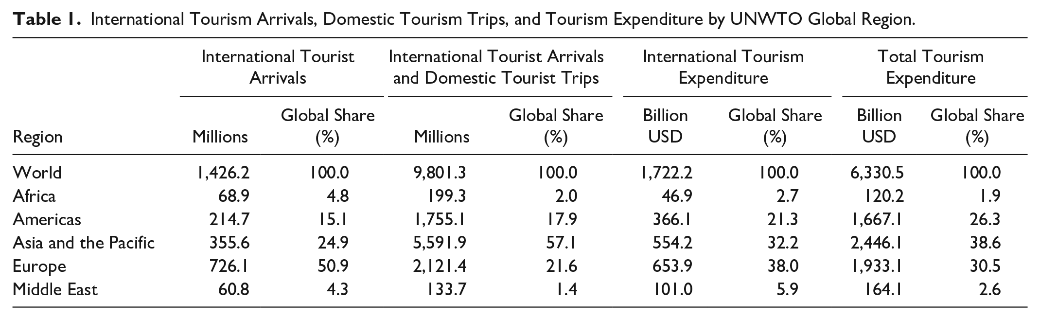
International tourism has a higher share in total tourism expenditure than in the number of tourist trips. Still, almost three quarters of global tourism spending is related to domestic travels. When expenditures are taken into account, the position of European and American countries is relatively higher than the number of visits: almost one third of total expenditures fall to European countries, which is only a little less than Asia and the Pacific.

The highest tourist traffic is observed in the countries with the highest populations. The 30 countries with the largest aggregate number of international tourist arrivals and domestic trips include 19 of the 30 most populated countries in the world (Table 2, Figure 2). In China and India, the number of tourists is twice as high as in the third country—the United States—and five to eight times as high as in the next countries—Japan, Russia, and France. In the countries with the highest numbers of tourist visits, domestic tourists predominate, and inbound tourists usually do not exceed 10% of the total. Only in European countries (e.g., France, Spain, and Germany) is the proportion of international tourists higher. On the other hand, tourism develops almost exclusively based on international tourists in many small and low-income countries of Africa, Antilles, and Oceania. A predominance of international visitors is also observed in the south-east of Europe (Albania, Croatia, Montenegro, Malta) and Arab states of the Persian Gulf.

Table 2.

Countries with the Largest Total Numbers of Total Tourism Visits and Largest Tourism Expenditure.

Tourism Visits (International Arrivals and Domestic Trips)				Tourism Expenditure
Country	Number (million)	Percent International	Per Capita	Country	Total (billion USD)	Percent International	Per 100 USD of GDP
1. China*	2,218.2	2.9	1.59	1. China	1,215.3	11.6	8.5
2. India	1,796.1	1.0	1.31	2. United States	1,103.6	20.5	5.2
3. United States*	1,001.9	7.9	3.05	3. Germany	451.2	13.1	11.7
4. Japan	343.5	9.3	2.72	4. India	283.0	12.7	9.8
5. Russia*	274.1	9.1	1.90	5. Japan	223.0	16.9	4.4
6. France	272.1	33.1	4.18	6. United Kingdom	220.4	17.9	7.8
7. Spain	249.5	33.5	5.30	7. Italy	218.9	24.2	10.9
8. Indonesia	213.9	7.2	0.79	8. France	202.9	29.1	7.7
9. Brazil	197.3	3.2	0.94	9. Mexico	165.5	17.0	13.0
10. Germany	192.3	20.6	2.31	10. Spain	155.9	56.8	11.2
11. Mexico*	183.9	22.7	1.44	11. Brazil	111.8	6.6	6.1
12. South Korea	174.0	10.1	3.36	12. Australia	110.8	22.8	7.9
13. Thailand	164.0	23.5	2.36	13. Thailand	91.4	80.5	16.8
14. United Kingdom	162.2	24.3	2.43	14. Canada	85.5	22.4	4.9
15. Malaysia	139.8	18.7	4.37	15. South Korea	76.9	27.5	4.7
16. Turkey	121.5	38.0	1.46	16. Turkey	75.9	53.6	10.0
17. Italy	118.8	54.3	1.97	17. Russia	64.8	26.3	3.9
18. Canada	112.9	18.9	3.00	18. Philippines	63.9	13.5	17.0
19. Australia	110.6	8.5	4.36	19. Hong Kong S.A.R.	55.3	77.3	15.1
20. Taiwan	68.7	17.3	2.91	20. Austria	53.0	47.2	11.9
21. Poland	65.5	30.2	1.73	21. Switzerland	50.6	43.8	7.2
22. Iran	64.5	11.4	0.78	22. United Arab Emirates	50.0	76.4	11.9
23. Philippines	61.6	13.4	0.57	23. Sweden	47.9	41.9	9.0
24. Saudi Arabia	61.4	22.2	1.79	24. Argentina	47.8	14.0	10.7
25. Vietnam	57.7	31.2	0.60	25. Netherlands	42.7	50.2	4.7
26. Argentina	50.6	13.8	1.13	26. Malaysia	41.5	51.7	11.4
27. Sweden	45.6	16.5	4.44	27. Indonesia	40.7	40.2	3.6
28. Peru	44.5	10.0	1.37	28. Macao S.A.R.	40.4	97.0	75.1
29. Austria	43.9	72.7	4.94	29. Taiwan*	39.0	43.6	6.4
30. Czechia	41.9	34.4	3.93	30. Saudi Arabia	34.6	43.5	4.4

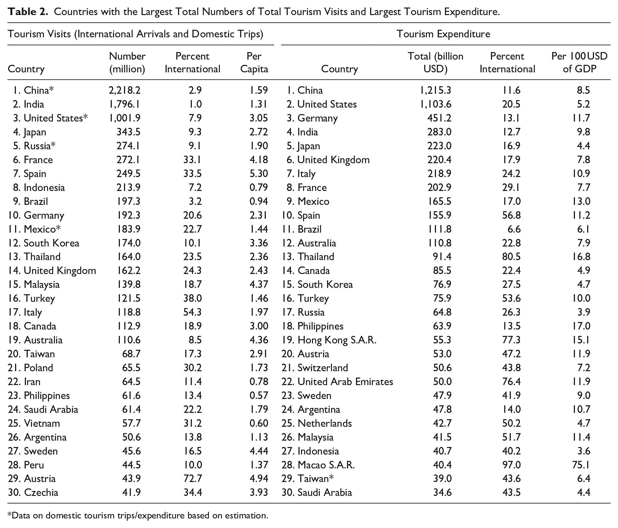
Data on domestic tourism trips/expenditure based on estimation.

Figure 2.

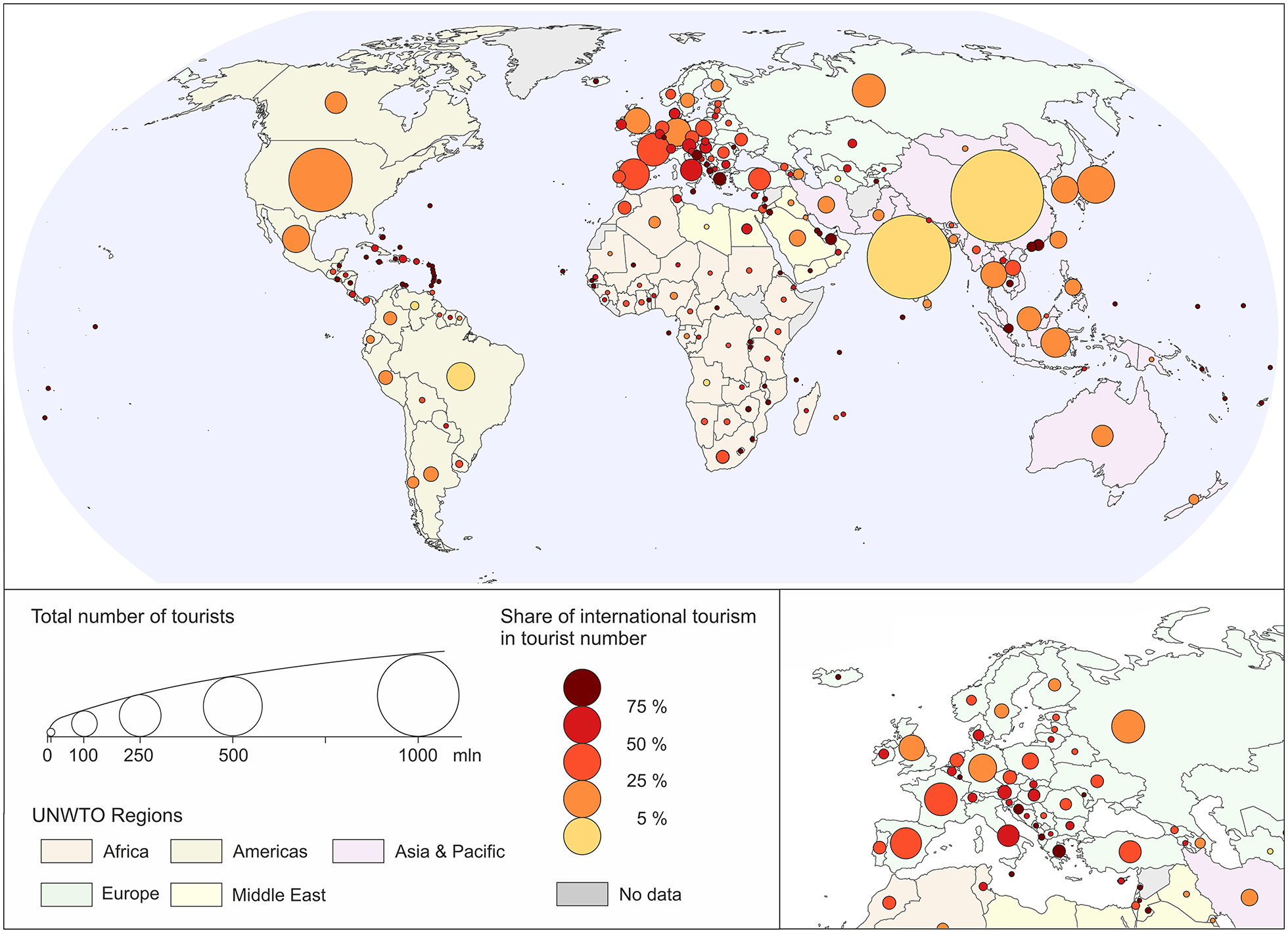
Numbers of international tourist arrivals and domestic tourist trips in countries.

The distribution of tourism expenditure does not directly correspond to the numbers of tourism visits (Table 2, Figure 3). While the USA and China are the leaders of both lists (tourists spent over a trillion dollars in each of these countries), in terms of tourism expenditures they are followed mostly by large Western European countries (Germany, the United Kingdom, Italy, and France). The share of international tourism in tourism expenditure is relatively high in South-East Asia, Southern Europe, and the Middle East, as well as the Caribbean countries and Africa.

Figure 3.

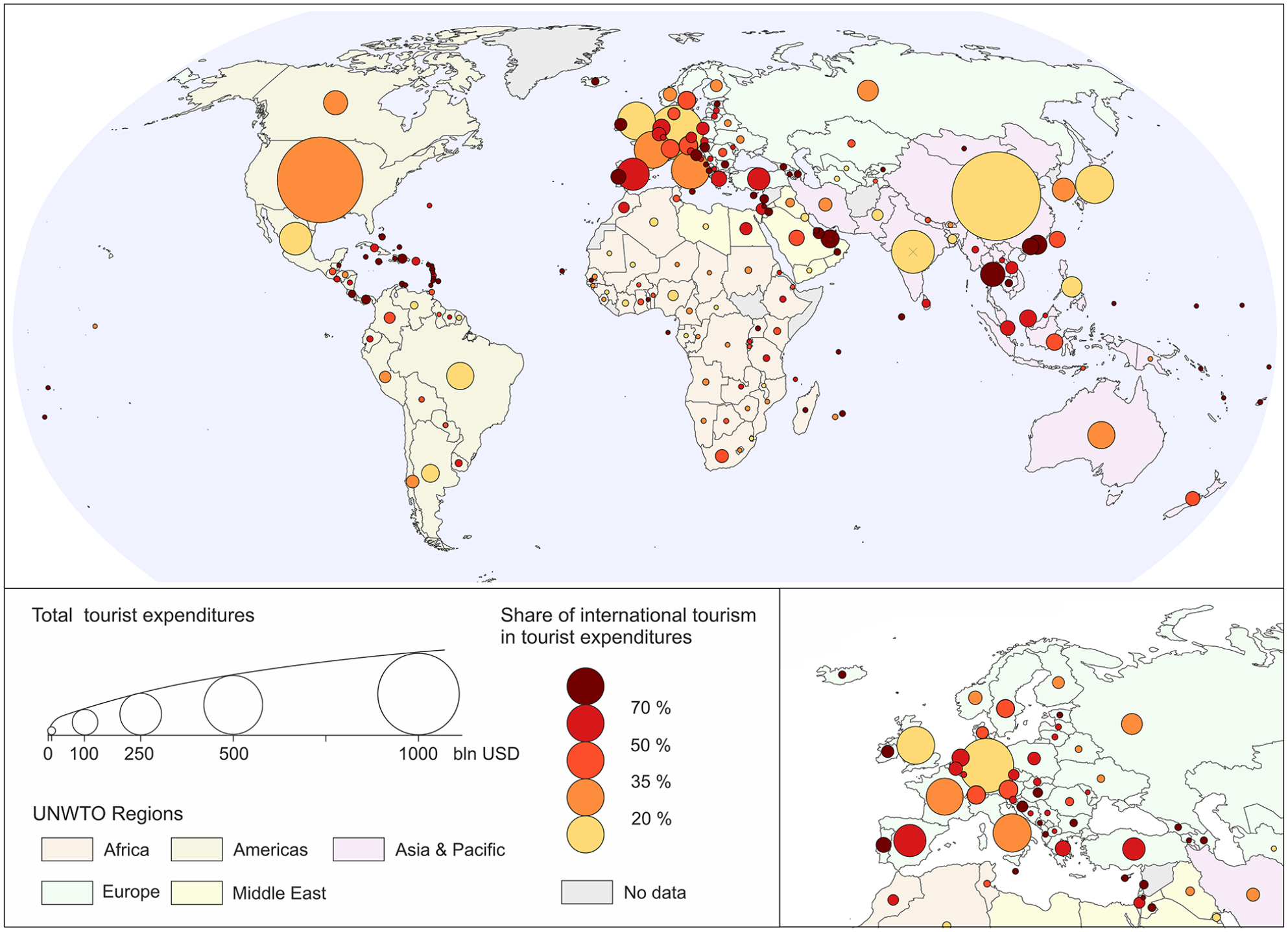
International and domestic tourism expenditure in countries.

Distribution of Tourism Visits and Expenditure in Grid Cells

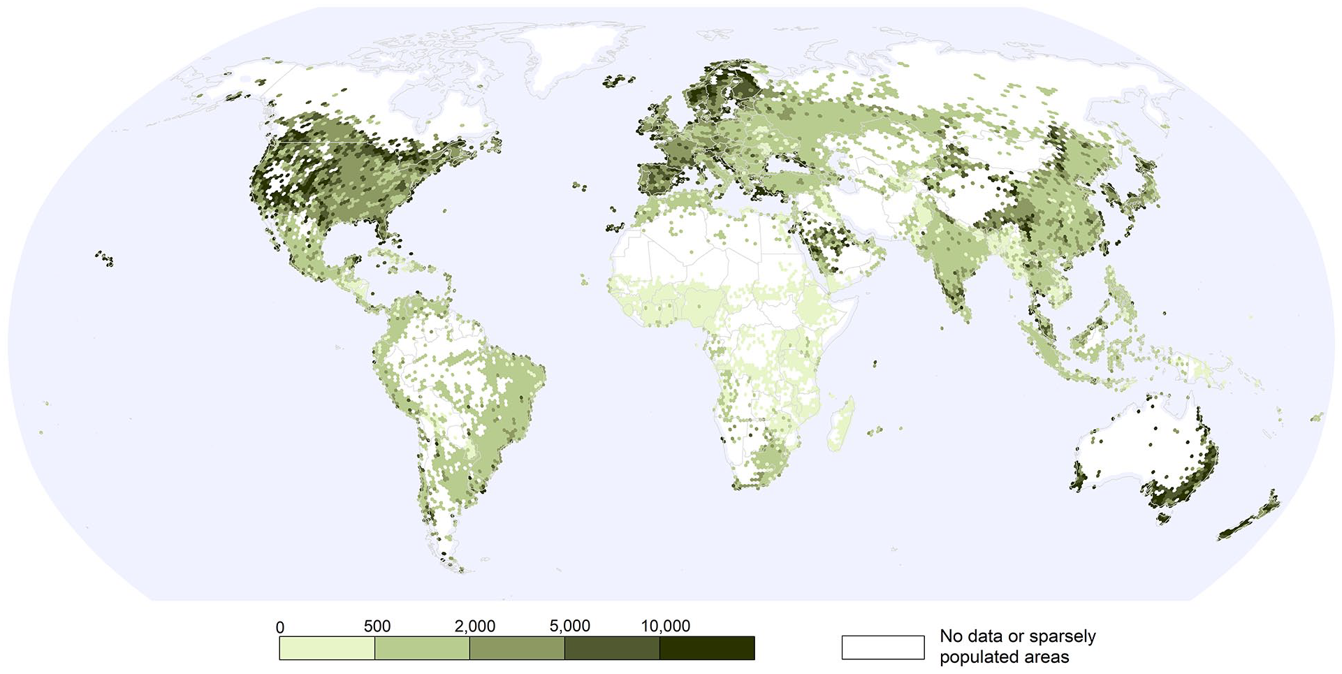
The analysis of the data on lower spatial scale of homogeneous geometric fields shows great variations in the density of tourism visits and expenditure within individual countries. Major concentrations of tourism visits are found in Europe, East Asia, and India (Figure 4). The highest tourist attendance is observed in large metropolises (not only national capitals) and their surroundings. Twenty-seven of the thirty most visited grid cells contain large Asian cities (12 in China [including Hong Kong and Macau]; 11 in India; as well as Seoul, Tokyo, Bangkok, and Jakarta; Table 3). In Europe, the largest number of tourists visit capital cities and grid cells on the Mediterranean coast and along the highly urbanized belt stretching from Northern Italy to England. In North America, the largest number of tourists visit the north-eastern megalopolis of the USA, California, Florida, central Mexico, and the Rio de Janeiro region. There are only minor tourism clusters in the African continent, for example, some grid cells located in South Africa, Egypt, Morocco, and Tunisia.

Figure 4.

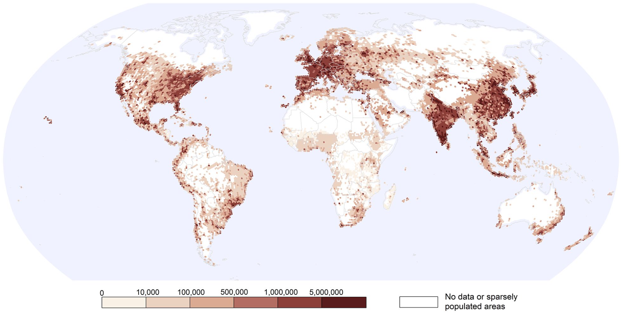
Total number of tourist visits in grid cells.

Table 3.

Grid Cells with the Highest Total Numbers of Tourist Visits, Highest Numbers of International Tourist Visits and Largest Tourism Expenditure.

Highest Number of Tourist Visits			Highest Number of International Tourist Visits			Highest Tourist Expenditure
	Major city within a Grid Cell (Countries Within a Grid Cell)	Total Number of Tourist Visits (Millions)		Major City within a Grid Cell (Countries Within a Grid Cell)	Number of Inbound Tourist Visits (Millions)		Major City within a Grid Cell (Countries Within a Grid Cell)	Total Tourism Expenditure (Billion USD)
1.	Hyderabad (India)	74.6	1.	Paris (France)	29.8	1.	Macau (Macau, China, Hong Kong)	71.3
2.	Chennai (India)	73.4	2.	Macau (Macau, China, Hong Kong)	27.6	2.	New York (USA)	50.2
3.	Shanghai (China)	67.1	3.	Bangkok (Thailand)	17.9	3.	Shanghai (China)	44.7
4.	Bengaluru (India)	56.9	4.	Singapore (Singapore, Malaysia)	16.7	4.	Paris (France)	39.7
5.	Delhi (India)	56.8	5.	Hong Kong (Hong Kong, China)	14.8	5.	Bangkok (Thailand)	37.9
6.	Moscow (Russia)	55.6	6.	Dubai (UAE)	14.6	6.	Berlin (Germany)	34.1
7.	Paris (France)	55.3	7.	Istanbul (Turkey)	13.7	7.	Tokyo (Japan)	33.9
8.	Beijing (China)	54.5	8.	Barcelona (Spain)	13.5	8.	Beijing (China)	33.8
9.	Guangzhou (China)	53.3	9.	London (UK)	13.3	9.	Guangzhou (China)	33.3
10.	Seoul (South Korea)	51.8	10.	Moscow (Russia)	12.2	10.	Singapore (Singapore, Malaysia)	32.0
11.	Tokyo (Japan)	49.3	11.	Budapest (Hungary, Slovakia)	11.2	11.	Hong Kong (Hong Kong, China)	31.7
12.	Macau (Macau, China, Hong Kong)	47.4	12.	Amsterdam (Netherlands)	10.2	12.	Los Angeles (USA)	30.3
13.	Coimbatore (India)	45.1	13.	Prague (Czechia)	9.4	13.	London (United Kingdom)	30.0
14.	Bangkok (Thailand)	44.8	14.	Antalya (Turkey)	9.0	14.	Dubai (United Arab Emirates)	29.2
15.	Chongqing (China)	43.3	15.	Kuala Lumpur (Malaysia)	8.4	15.	Washington (USA)	27.4
16.	Jakarta (Indonesia)	41.3	16.	Venice (Italy)	8.3	16.	Chongqing (China)	27.3
17.	Agra (India)	40.9	17.	Innsbruck (Austria, Germany, Italy)	8.1	17.	Munich (Germany)	26.1
18.	Theni (India)	40.2	18.	Copenhagen (Denmark, Sweden)	8.1	18.	Hamburg (Germany)	25.4
19.	Varanasi (India)	37.6	19.	Vienna (Austria)	7.8	19.	Frankfurt am Main (Germany)	25.1
20.	Kolkata (India)	37.2	20.	Tokyo (Japan)	7.7	20.	Las Vegas (USA)	25.1
21.	Chengdu (China)	36.4	21.	Seoul (South Korea)	7.7	21.	Seoul (South Korea)	25.0
22.	Hangzhou (China)	35.7	22.	Madrid (Spain)	7.6	22.	Chengdu (China)	22.1
23.	Puducherry (India)	34.3	23.	New York (USA)	7.5	23.	Shenzhen (China, Hong Kong)	22.0
24.	Deyang (China)	34.2	24.	Rome (Italy)	7.4	24.	Hangzhou (China)	21.7
25.	Mumbai (India)	33.6	25.	Mexico City (Mexico)	7.3	25.	Osaka (Japan)	21.7
26.	Suzhou (China)	33.4	26.	Palma (Spain)	7.2	26.	Köln (Germany, Belgium, Netherlands)	21.7
27.	Xiamen (China, Taiwan)	32.8	27.	Ho Chi Minh (Vietnam)	6.8	27.	Deyang (China)	20.8
28.	Wuhan (China)	32.4	28.	Shanghai (China)	6.5	28.	Kyoto (Japan)	20.2
29.	Shenzhen (China, Hong Kong)	31.6	29.	Kyiv (Ukraine)	6.3	29.	Xiamen (China, Taiwan)	20.1
30.	New York (USA)	31.5	30.	Cairo (Egypt)	6.2	30.	Barcelona (Spain)	19.9

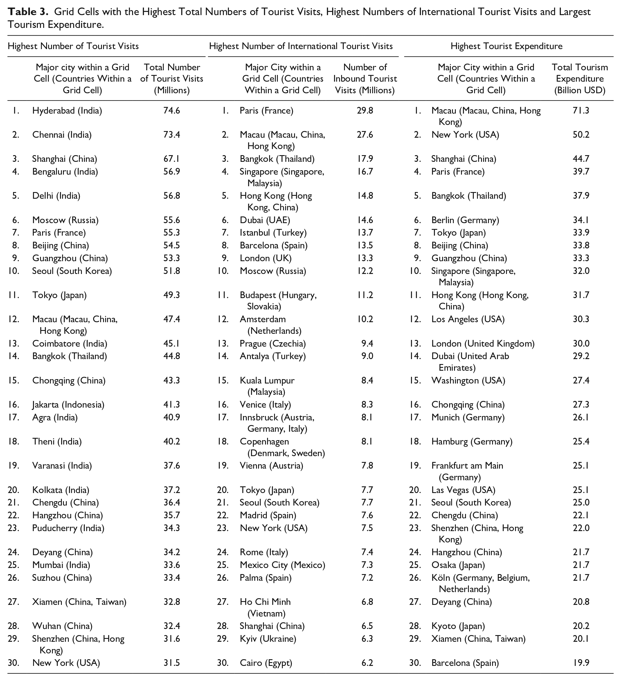
International tourism visits are evidently more concentrated in Europe, while the relative position of Mainland China and India is lower (Figure 5). The group of 30 grid cells most frequently visited by foreign tourists includes 11 European capitals and six other tourist destinations in Europe (including Turkey). Apart from major cities, they also include leisure destinations in the Mediterranean region (Antalya, Palma) and the Alps (Innsbruck; Table 3). In Asia and the Middle East, Macau, Hong Kong, Bangkok, Singapore, and Dubai are among the top international tourism destinations. Ignoring domestic tourism also elevates the relative position of Central America, the Caribbean, and South-East Asia.

Figure 5.

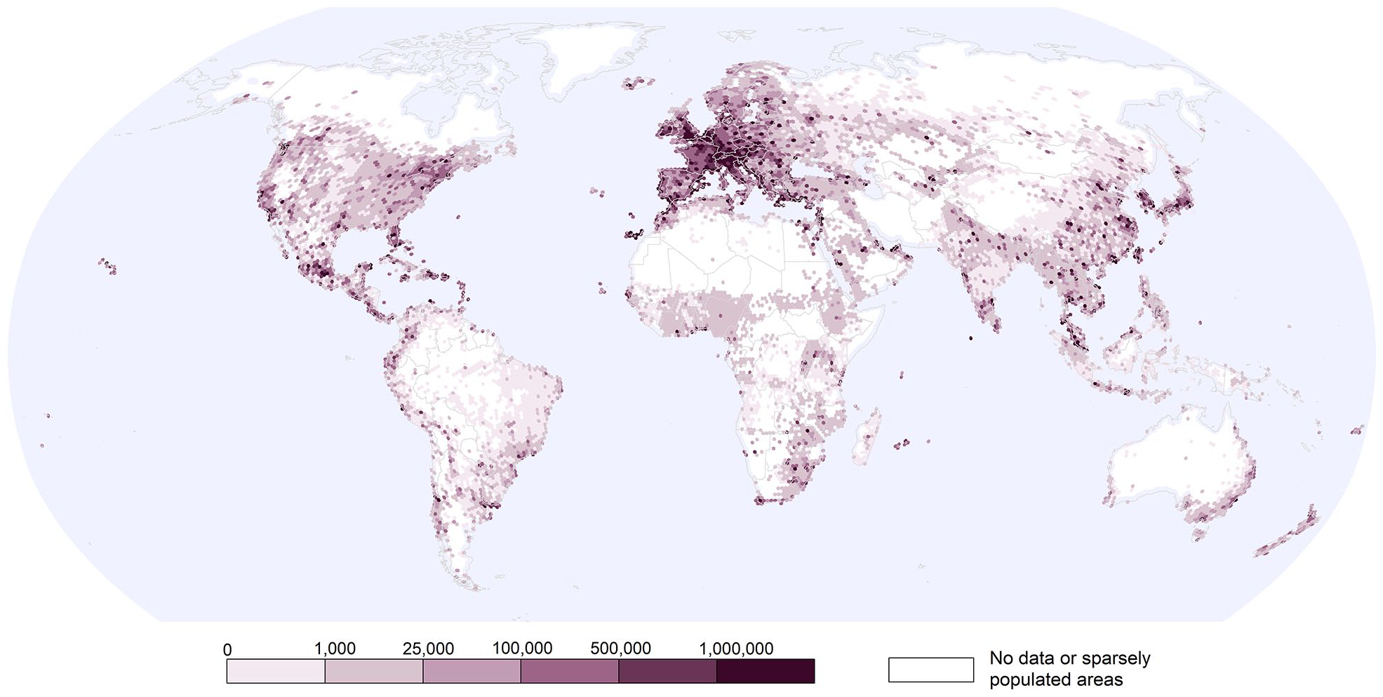
Number of international tourist visits in grid cells.

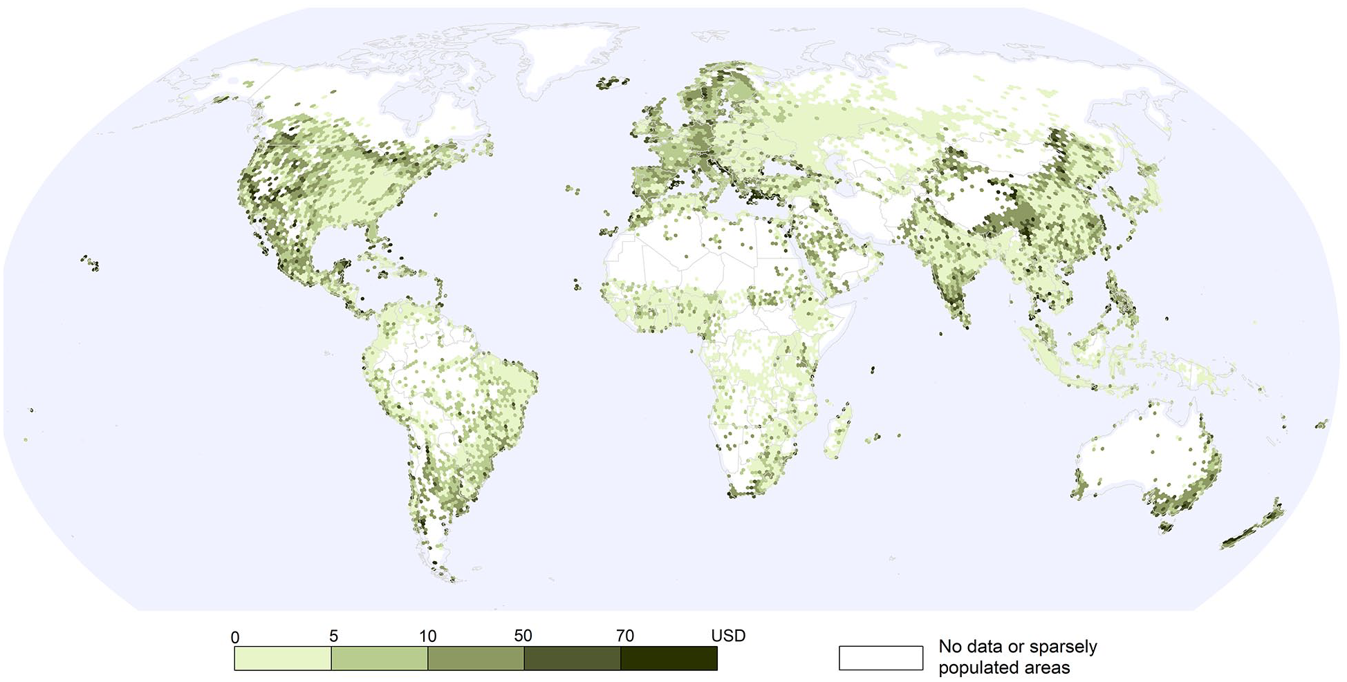
The distribution of tourism expenditure depends not only on the number of tourist visits, but also on the level of economic development of a given region, which also translates into the cost of living. Hence the high position of north-western and Alpine Europe, East Asia, and urbanized parts of the United States (Figure 6). Grid cells with the highest amounts of money spent by tourists include major European and Asian metropolises (particularly the ones often visited by international tourists), as well as major North American and Middle Eastern destinations (Table 3).

Figure 6.

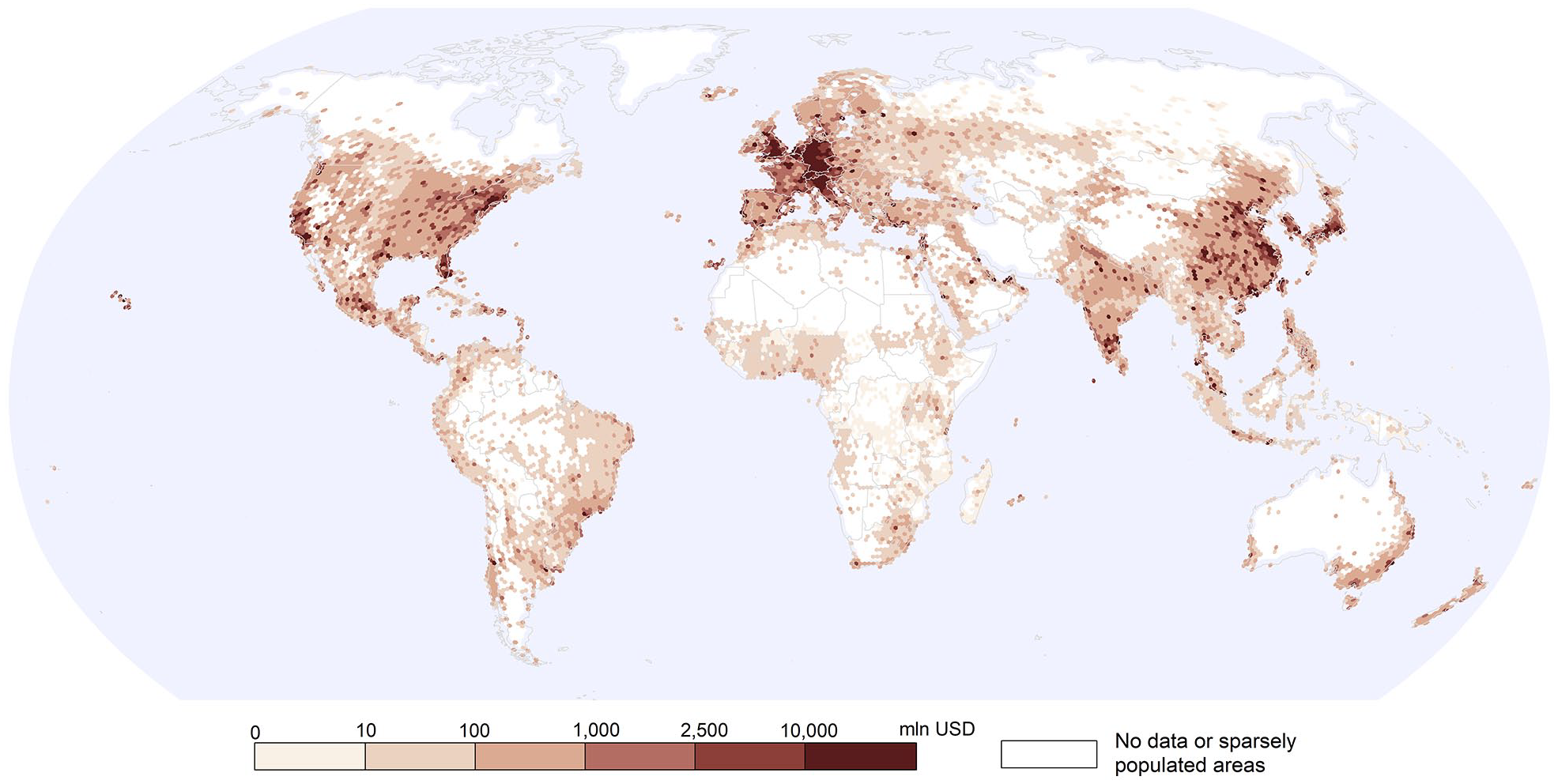
Tourism expenditure in grid cells.

Figures 7 and 8 present the spatial variation of the intensity of tourism relative to the size of local population and economy. Unlike what can be seen on Figures 4 and 5, they do not follow the global distribution of population and economic product. Europe retains high values, along with North America, Australia, and New Zealand. Regional differences are explained by the access to leisure amenities: sea (in Europe, coasts of China, and North America), mountains (the Alps, the Rocky Mountains, Yunnan, and Sichuan provinces), and favorable climatic conditions (areas to the south of major population concentrations in the northern hemisphere). Apart from primary world destinations, a high ratio of tourists per population characterises regions with relatively low population densities but high tourist activity of local residents, for example, the Nordic countries.

Figure 7.

Tourism visits per 1,000 inhabitants in grid cells.

Figure 8.

Tourism expenditure per 100 USD of GDP in grid cells.

When relative importance of tourism for local economy is measured, southern Europe, Central America and the Carribean as well as parts of South-East Asia stand out. In the Middle East, coastal resorts on the Red Sea and cities on the southern coast of the Persian Gulf are characterised by high relative tourism numbers and expenditures. Moreover, island locations are often particularly tourism-intensive, including European islands (the Balearic Islands, Canary Islands, Greek and Croatian Islands, and Iceland), Hawaii, Maldives, and New Zealand.

World maps presented in Figures 4 to 8 are too general to read the patterns of presented variables on the regional or national scale, so a more detailed supplementary map is attached to the article. A section of this map is demonstrated in Figure 9. Semicircle sizes are proportional to the numbers of tourists visiting a given grid cell (left semicircles) and tourism expenditure (right semicircles). The color tint displays the intensity of tourism, while color hue informs about the share of international tourists in total tourism visits and expenditure. Apart from this map, borders of grid cells and basic indicators of tourism intensity may be consulted on a web map (http://puma.uci.umk.pl/~czeslaw/global-destinations/), and a shapefile with the resulting dataset (hexagons.shp) is provided as a Supplemental File for further re-use.

Figure 9.

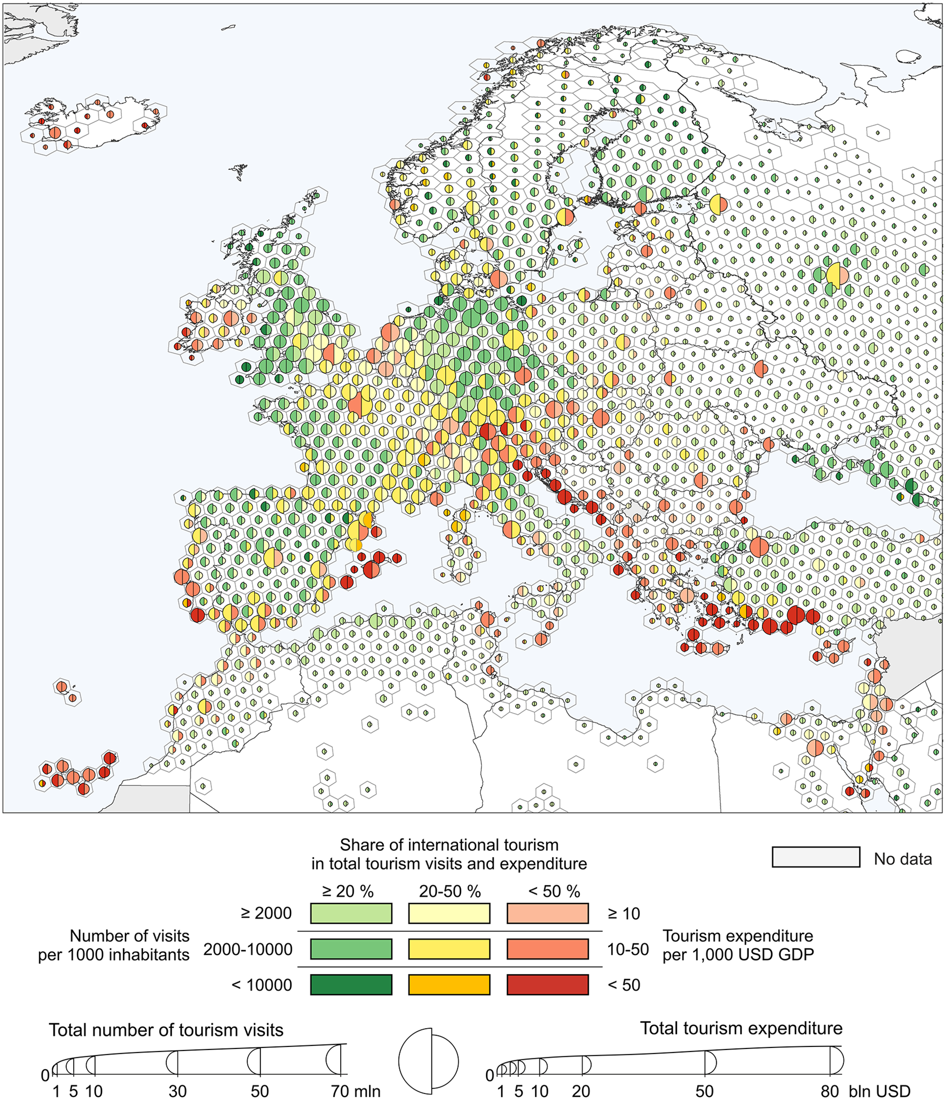
Fragment of World map of tourism destinations (printed version contains a simplified figure—see online version for the full version; entire map in Supplemental File).

Hotspots of Global Tourism

Hotspot analysis provides a generalized image of the territorial variation in tourism size and intensity (Figure 10). Out of four major clusters of tourism visits (Europe, East Asia, India, and western North America) only Europe is also a large hotspot of international tourism. Smaller hotspots exist in various parts of the world—mainly East and South-East Asia and North America. When tourism expenditure is measured instead of the number of visits, eastern North America takes the place of India as the third global concentration. Low tourism numbers and expenditures are clustered in central Africa and also, with regard to foreign tourists, in Asia.

Figure 10.

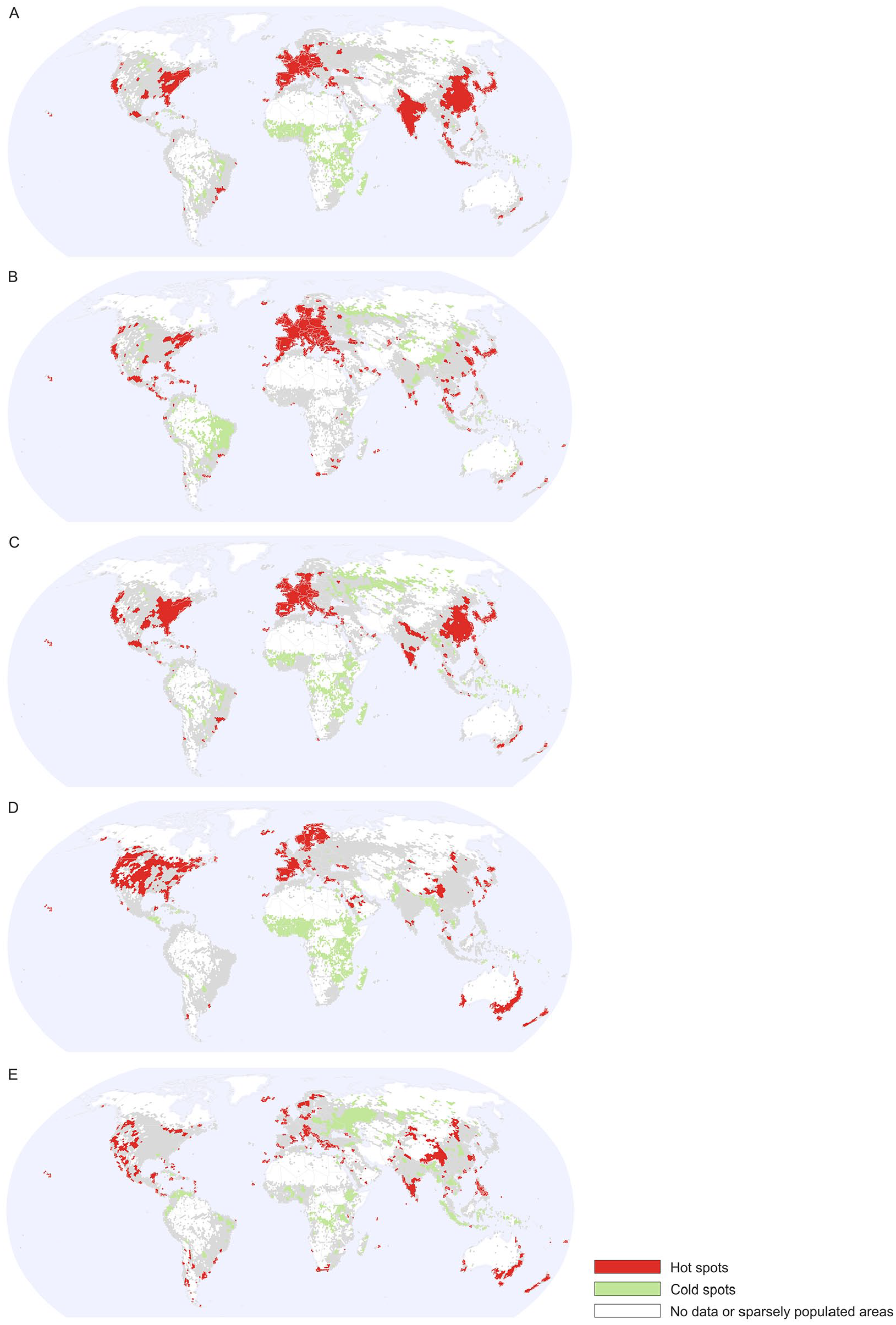
Hotspots and cold spots of tourism in hexagonal grid cells: (A) Total tourism visits. (B) Visits of international tourists. (C) Total tourism expenditure. (D) Tourist visits per population. (E) Tourist expenditure per GDP.

This pattern changes when the intensity of tourism is presented in relative terms. Clusters of high tourism visits per capita are present mostly in Europe, North America, Australia, and New Zealand, thanks to high numbers of domestic and short-distance international tourism trips. Hotspots of tourism intensity measured in monetary terms are more dispersed and located away from the core areas of the global economy: on the Mediterranean coasts, in Central, South-East and Southern Asia, as well as in Central America and western North America. Again, in most regions of Central Africa, tourism does not play an important role, even in relation to the total economy.

Global Concentration of Tourism

The Lorenz curves and Gini coefficients presented in Figure 11 were elaborated only based on the 9,601 grid cells after excluding those located on sparsely populated areas. Still, over half of the population and two thirds of the economic productivity is concentrated in just 10% of the area of these grid cells. The distribution of tourism visits turns out to be more spatially concentrated than the distribution of population. Tourism expenditure is also slightly less dispersed over the territory than general economic product. The global distribution of international travels is substantially more concentrated on small territories than domestic tourism mobility, both in terms of the number of visits and expenditure.

Figure 11.

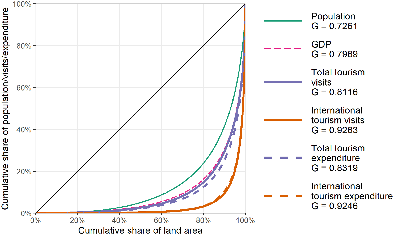
Lorenz curves and Gini coefficients presenting the concentration of tourism in grid cells.

Discussion

The study aimed to map and describe the distribution of global tourism destinations with more spatial detail than using conventional statistics. This was done by employing novel big-data sources: gridded population database and geo-referenced data on Airbnb accommodation offers. The resulting maps enable comparison of the total and relative numbers of tourist visits and tourism expenditure in geometric grid cells covering most countries of the world. The maps confirm that the distribution of tourism is a resultant of the distribution of demand (population and its purchasing power) and supply (natural amenities and tourism resorts). The maps of absolute number of tourist visits and total tourism expenditure roughly correspond to the maps of total population and economic product, respectively. If relative instead of absolute values are considered, semi-peripheral locations not too distant from the major population and economic centers and offering favorable natural conditions stand out.

Apart from confirming the established knowledge, the results help to confront some common misconceptions about the spatial patterns of global tourism. First, they emphasize the dominant role of domestic tourism in the structure of global tourism flows. Domestic trips are not only the vast majority (85%) of total tourist travels, but they also account for three-quarters of the global tourism economy. The distribution of domestic destinations often differs from the distribution of international destinations within a country, and domestic trips tend to be more dispersed over the territory of a country than inbound visits. Despite the growing number of geographical studies acknowledging the importance of domestic tourism (Rogerson 2015), it is still often considered less important than international travels not least because of the difference in the availability of statistical data (Peeters and Landré 2011). Second, considering both international and domestic tourism reduces the perceptual dominance of Europe, or more generally of high-income countries, on the global map of tourism. Their share in tourism mobility and economy is considerable smaller than that of the aggregated middle-income countries of Asia (including China and India), the Americas, Eastern Europe, and the Middle East. Low-income countries in Africa and Asia, apart from small areas (often islands) turn out to be tourism cold spots. This means that, first, tourism demand and economy follow the national income along an S-shaped curve, and second, that with growing economy tourism tends to disperse over the territories of countries.

The study adds depth and detail to the conventional tourism statistics, yet it still inherits some of their limitations. First, the two measures of tourism that are used: the number of visits and expenditure, do not sufficiently describe the complexity of tourism behaviors and impacts. Tourists can stay at a destination for varied lengths of time, so the number of nights is often a better measurement of the volume of tourism than the number of visits. Taking into account the number of nights spent by tourists instead of the number of visits would probably reduce the relative position of capital cities, which are often destinations for short business trips, and increase the position of coastal and mountain destinations visited for longer leisure stays. In the case of the second measure—tourist expenditure—the problem of localizing economic impact arises: we assumed that the entire expenditure is bound to the destination, while in fact, for example, the cost of transportation may be incurred in other locations. Evaluating and localizing the total economic impact of tourism would require the analysis of both the supply and demand for goods and services associated with tourism activity. Such perspective is a basis of tourist satellite accounts, which are usually evaluated for the entire countries, and the possibility of their international comparisons, even on the European Union level, is very limited (Eurostat 2019). Also, tourism statistics are usually based on tourism accommodation statistics, and a large part of tourism stays remain unobserved (De Cantis et al. 2015), including stays: in second homes (Müller and Hall 2018), with friends and relatives (Jackson 1990), and in informal accommodation establishments, including peer-to-peer accommodation (Guttentag 2015). Differences in national methodologies of tourism statistics result in limitations in the comparability of the data about the numbers of both international arrivals (e.g., differences between countries measuring arrivals at frontiers and at accommodation establishments) and domestic trips. Comparing the reported numbers of domestic trips with predictions of the model used for extrapolating the missing data gives some idea about the extent of such bias. For example, the reported numbers of domestic trips are extremely low compared to the estimation in some Eastern and Southern European countries (e.g., Belarus—2.5 times lower, Italy—2.4 times lower), while they are much higher in India (5 times), Finland (2.2 times), and Czechia (2 times). This may well be a result of specific factors not measured by the model, but may also stem from data incompatibility.

The second source of the limitations is the employed procedure of disaggregating tourism visits into smaller territorial units. We assumed that each tourist trip is directed only to a single destination, while in fact a tourist may visit multiple places during one trip. This means that our dataset may underrate the number of visits in grid cells, particularly international visits in large countries. We decided on the size of reference grid cells as a trade-off between larger grid cells producing more robust estimations and the greater detail offered by smaller cells. In Europe this size of grid cells may appear large (e.g., Batista e Silva et al. 2018, used 100 × 100-m grid cells for the dataset and presented the results at 10 × 10-km resolution), yet it enables the entire world to be covered and legible world maps to be designed. Finally, the formula for disaggregating the numbers of tourists and tourism expenditures into grid cells was evaluated based on European data and it is not obvious that it is appropriate to other parts of the world. To verify the validity of this estimation, we confronted our results concerning the distribution of international visits in China with official Chinese statistics on international tourist visits to province-level administrative divisions of the country (National Bureau of Statistics of China 2019; we did not use this data in the first step of the analysis due to the lack of official data on the provincial distribution of domestic visits). We assumed that the distribution of tourism within each grid cell is constant over territory, so part of the error results from the provincial borders intersecting grid cells. Still, in most provinces the difference between the estimated and actual numbers of international tourist arrivals is lower than 50% (Figure 12). High discrepancy only pertained to provinces with low absolute numbers of international tourism visits (bottom left corner of the chart).

Figure 12.

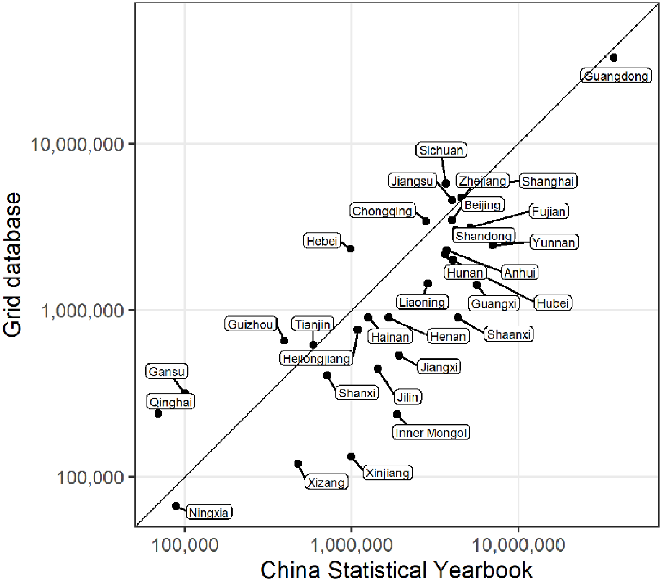
Estimation of international tourism arrivals to provincial-level administrative divisions of China compared with the national statistics.

From the perspective of destination management and tourism policy, the results may help more informed planning of tourism development on large territorial scales. The predominance of domestic tourism and common locational difference between domestic and international tourism destinations support the idea that, particularly in middle-income countries, tourism development should be directed to the domestic, and not only international market, to obtain a territorially balanced distribution of its economic benefits (Rogerson 2015; Seckelmann 2002; UNWTO 2020a). Considering the challenges of mitigating climate change and the growing contribution of tourism mobility, particularly long-haul air travel, to greenhouse gas emissions, the current research gives support to the claim that global tourism development is not inherently dependent on long-haul travel and could develop on the basis of shorter trips with the use of ground transportation (Peeters and Eijgelaar 2014; Peeters and Landré 2011). A detailed map of tourism destinations may also help to add precision to the evaluation of the future impacts of climate change (Scott, Hall, and Gössling 2019). Many global tourism clusters are located in the parts of the world particularly endangered by increasing water deficits and more frequent extremely hot days (e.g., Mediterranean coasts, Caribbean and Central America, southern China, islands in the tropical zone; IPCC 2018, 2020).

The results of the current study may also help monitor the territorial effects of the COVID-19 pandemics. Tourism has been among the sectors of the economy most affected by the spread of the pandemic and the non-pharmaceutical interventions employed to contain it (Gössling, Scott, and Hall 2021). These impacts have varied geographically between and within countries (UNWTO 2021b; Yang et al. 2021). Due to border closures, international tourism was particularly affected (UNWTO estimates international tourism to have fallen by 74% in 2020 compared to the previous year), while domestic and proximity tourism is expected to recover more quickly (Romagosa 2020; UNWTO 2020a; Zenker and Kock 2020). The reduction in international mobility may be long-term due to continuous administrative and economic constraints, perceived barriers, and structural changes in the tourism industry. The current study identifies areas particularly economically dependent on tourism in general and on international tourism in particular, which may help forecast the future development of tourism destinations in the post-COVID reality.

The presented study belongs to a growing body of research employing big-data sources to analyze the spatial patterns of tourism. Such an approach has been extensively developed during the pandemic as it enables tracking dynamic changes in a near-real-time manner. Booking data, Internet searches, user-generated data, and mobile device data have been used for monitoring the situation in passenger transportation, hotel and short-term rental markets (Gallego and Font 2021; Gössling et al. 2021; Napierała, Leśniewska-Napierała, and Burski 2020; Nhamo, Dube, and Chikodzi 2020; Yang et al., 2021). The method used in the current study may contribute to this development, and two avenues of its development seem particularly promising. First, repeating similar studies in the future will be useful to explore the time trend, for example, global changes in the level of concentration of tourism on general spatial scale (Lacher and Nepal 2013) and changes in the location of major tourism hotspots. The current pandemic may accelerate such changes, as, apart from the short-term impacts, long-term processes are hypothesized to occur, for example, changes in destination images, development of peripheral tourism destinations at the cost of central ones, reduction in business trips, shift of transport modes toward private cars, or new more sustainable paths of destination and business development (Li, Nguyen, and Coca-Stefaniak 2020; Niewiadomski 2020; Zenker and Kock 2020). The second possible development of the method is to include the origin of tourism travels in the database. Considering tourism origins, destinations, and transit routes may enable, for example, disaggregation of the contribution that tourist travels to specific destinations make to greenhouse gas emissions (Peeters and Landré 2011). In the post-COVID context, it may also help to track the long-term changes in travel behavior, for example, the pace of return of international mobility. Mapping tourism origins could be based on user-generated content on Internet platforms and later estimations considering location and level of urbanization.

Supplemental Material

sj-7z-1-jtr-10.1177_00472875211051418 – Supplemental material for Combining Conventional Statistics and Big Data to Map Global Tourism Destinations Before COVID-19

Supplemental material, sj-7z-1-jtr-10.1177_00472875211051418 for Combining Conventional Statistics and Big Data to Map Global Tourism Destinations Before COVID-19 by Czesław Adamiak and Barbara Szyda in Journal of Travel Research

Supplemental Material

sj-7z-2-jtr-10.1177_00472875211051418 – Supplemental material for Combining Conventional Statistics and Big Data to Map Global Tourism Destinations Before COVID-19

Supplemental material, sj-7z-2-jtr-10.1177_00472875211051418 for Combining Conventional Statistics and Big Data to Map Global Tourism Destinations Before COVID-19 by Czesław Adamiak and Barbara Szyda in Journal of Travel Research

Supplemental Material

sj-png-3-jtr-10.1177_00472875211051418 – Supplemental material for Combining Conventional Statistics and Big Data to Map Global Tourism Destinations Before COVID-19

Supplemental material, sj-png-3-jtr-10.1177_00472875211051418 for Combining Conventional Statistics and Big Data to Map Global Tourism Destinations Before COVID-19 by Czesław Adamiak and Barbara Szyda in Journal of Travel Research

Footnotes

Appendix

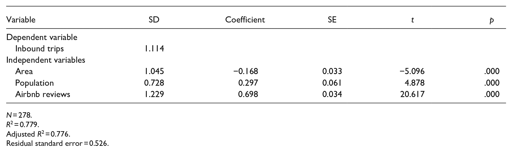
Variable	SD	Coefficient	SE	t	p
Dependent variable
Inbound trips	1.114
Independent variables
Area	1.045	−0.168	0.033	−5.096	.000
Population	0.728	0.297	0.061	4.878	.000
Airbnb reviews	1.229	0.698	0.034	20.617	.000

N = 278.

R² = 0.779.

Adjusted R² = 0.776.

Residual standard error = 0.526.

Declaration of Conflicting Interests

The author(s) declared no potential conflicts of interest with respect to the research, authorship, and/or publication of this article.

Funding

The author(s) received no financial support for the research, authorship, and/or publication of this article.

ORCID iD

Czesław Adamiak

Supplemental Material

Supplemental material for this article is available online.

Author Biographies

Czesław Adamiak, PhD in geography, is an adjunct at the Faculty of Earth Sciences and Spatial Management and a member of the University Centre of Excellence IMSErt - Interacting Minds, Societies, Environments, at the Nicolaus Copernicus University in Toruń. His research interests include tourism geography, regional development, and the applications of geographic information systems and big data in social sciences. His current research focus on role of online peer-to-peer rental platforms in tourism behaviour and the evolution of tourism destinations.

Barbara Szyda, PhD in geography, works at the Faculty of Earth Sciences and Spatial Management, Nicolaus Copernicus University in Toruń. Her research interests are related to local socio-economic development, particularly of rural areas, and changes of human and social capital.

References

Abrahamson

2004. Global Cities. New York, NY: Oxford University Press.

Adamiak

2019. “Current State and Development of Airbnb Accommodation Offer in 167 Countries.” Current Issues in Tourism. Published online December 4. doi:10.1080/13683500.2019.1696758.

Adamiak

Szyda

Dubownik

García-Álvarez

2019. “Airbnb Offer in Spain — Spatial Analysis of the Pattern and Determinants of Its Distribution.” ISPRS International Journal of Geo-Information 8:155. doi:10.3390/ijgi8030155.

Airbnb. 2020. “About Us.” May 12. https://press.airbnb.com/about-us/ (accessed May 12, 2020).

Aitchison

1986. The Statistical Analysis of Compositional Data. London: Chapman & Hall.

Barnes

2018. “dggridR: Discrete Global Grids. R package version 2.0.6.” https://github.com/r-barnes/dggridR/.

Batista e Silva

Marín Herrera

M. A.

Rosina

Ribeiro Barranco

Freire

Schiavina

2018. “Analysing Spatiotemporal Patterns of Tourism in Europe at High-Resolution with Conventional and Big Data Sources.” Tourism Management 68:101–15. doi:10.1016/j.tourman.2018.02.020.

Bauder

2019. “Engage! A Research Agenda for Big Data in Tourism Geography.” In A Research Agenda for Tourism Geographies, edited by Müller

D. K.

149–57. Cheltenham: Elgar.

Bigano

Hamilton

J. M.

Lau

Tol

R. S. J.

Zhou

2007. “A Global Database of Domestic and International Tourist Numbers at National and Subnational Level.” International Journal of Tourism Research 9 (3): 147–74. doi:10.1002/jtr.602.

10.

Bivand

R. S.

Wong

D. W. S.

2018. “Comparing Implementations of Global and Local Indicators of Spatial Association.” TEST 27 (3): 716–48. doi:10.1007/s11749-018-0599-x.

11.

Brouder

Clavé

S. A.

Gill

Ioannides

, eds. 2017. Tourism Destination Evolution. Abindgon: Routledge.

12.

Butler

R. W.

1980. “The Concept of a Tourist Area Life Cycle of Evolution: Implications for Management of Resources.” The Canadian Geographer/Le Géographe Canadien 24 (1): 5–12. doi:10.1111/j.1541-0064.1980.tb00970.x.

13.

Chen

Becken

Stantic

2021. “Using Weibo to Track Global Mobility of Chinese Visitors.” Annals of Tourism Research 89:103078. doi:10.1016/j.annals.2020.103078.

14.

Christaller

1964. “Some Considerations of Tourism Location in Europe: The Peripheral Regions-Under-Developed Countries-Recreation Areas.” Papers of the Regional Science Association 12 (1): 95–105. doi:10.1007/BF01941243.

15.

De Cantis

Parroco

A. M.

Ferrante

Vaccina

2015. “Unobserved Tourism.” Annals of Tourism Research 50:1–18. doi:10.1016/j.annals.2014.10.002.

16.

Deville

Linard

Martin

Gilbert

Stevens

F. R.

Gaughan

A. E.

Blondel

V. D.

Tatem

A. J.

2014. “Dynamic Population Mapping Using Mobile Phone Data.” Proceedings of the National Academy of Sciences 111 (45): 15888–93. doi:10.1073/pnas.1408439111.

17.

Dolnicar

, ed. 2018. Peer-to-Peer Accommodation Networks: Pushing the Boundaries. Oxford: Goodfellow Publishers.

18.

Eurostat. 2017. “Tourism Statistics: Early Adopters of Big Data? 2017 Edition.” https://op.europa.eu/en/publication-detail/-/publication/aaecb8d2-a19c-11e7-b92d-01aa75ed71a1/language-en (accessed October 4, 2021).

19.

Eurostat. 2019. “Tourism Satellite Accounts in Europe. 2019 Edition.” https://ec.europa.eu/eurostat/documents/7870049/10293066/KS-FT-19-007-EN-N.pdf/f9cdc4cc-882b-5e29-03b1-f2cee82ec59d?t=1575909526000 (accessed June 24, 2021).

20.

Eurostat. 2020a. “Database.” https://ec.europa.eu/eurostat/web/regions/data/database (accessed November 9, 2020).

21.

Eurostat. 2020b. “NUTS.” https://ec.europa.eu/eurostat/web/gisco/geodata/reference-data/administrative-units-statistical-units/nuts (accessed November 9, 2020).

22.

Federal State Statistic Service. 2021a. “Численность иностранных граждан, размещенных в коллективных средствах размещения [The number of foreign citizens accommodated in collective accommodation facilities].” https://showdata.gks.ru/report/280009/ (accessed February 4, 2021).

23.

Federal State Statistic Service. 2021b. “Численность граждан Российской Федерации, размещенных в коллективных средствах размещения [The number of citizens of the Russian Federation accommodated in collective accommodation facilities].” https://showdata.gks.ru/report/280007/ (accessed February 4, 2021).

24.

Fradkin

Grewal

Holtz

2018. “The Determinants of Online Review Informativeness: Evidence from Field Experiments on Airbnb.” SSRN Electronic Journal. doi:10.2139/ssrn.2939064.

25.

Gallego

Font

2021. “Changes in Air Passenger Demand as a Result of the COVID-19 Crisis: Using Big Data to Inform Tourism Policy.” Journal of Sustainable Tourism 29 (9): 1470–89. doi:10.1080/09669582.2020.1773476.

26.

Getis

Ord

J. K.

1992. “The Analysis of Spatial Association by Use of Distance Statistics.” Geographical Analysis 24 (3): 189–206. doi:10.1111/j.1538-4632.1992.tb00261.x.

27.

Goldberg

1934. “A Class of Multi-Symmetric Polyhedra.” Tohoku Mathematical Journal, First Series 43:104–8. https://www.jstage.jst.go.jp/article/tmj1911/43/0/43_0_104/_article

28.

Gómez Martín

M. B.

2005. “Weather, Climate and Tourism a Geographical Perspective.” Annals of Tourism Research 32 (3): 571–91. doi:10.1016/j.annals.2004.08.004.

29.

Gössling

Scott

Hall

C. M.

2021. “Pandemics, Tourism and Global Change: A Rapid Assessment of COVID-19.” Journal of Sustainable Tourism 29 (1): 1–20. doi:10.1080/09669582.2020.1758708.

30.

Government of India. 2018. “India Tourism Statistics, 2018.” https://tourism.gov.in/sites/default/files/2020-04/IndiaTourismStatistics2018_0.pdf (accessed October 4, 2021).

31.

Greer

Wall

1979. “Recreational Hinterlands: A Theoretical and Empirical Analysis.” Publication Series, Department of Geography, University of Waterloo 14:227–246.

32.

Gunter

Önder

2016. “Forecasting City Arrivals with Google Analytics.” Annals of Tourism Research 61:199–212. doi:10.1016/j.annals.2016.10.007.

33.

Gutiérrez

García-Palomares

J. C.

Romanillos

Salas-Olmedo

M. H.

2017. “The Eruption of Airbnb in Tourist Cities: Comparing Spatial Patterns of Hotels and Peer-to-Peer Accommodation in Barcelona.” Tourism Management 62:278–91. doi:10.1016/j.tourman.2017.05.003.

34.

Guttentag

2015. “Airbnb: Disruptive Innovation and the Rise of an Informal Tourism Accommodation Sector.” Current Issues in Tourism 18 (12): 1192–217. doi:10.1080/13683500.2013.827159.

35.

Hall

C. M.

2005. “Reconsidering the Geography of Tourism and Contemporary Mobility.” Geographical Research 43 (2):125–39. doi:10.1111/j.1745-5871.2005.00308.x.

36.

Hall

M. C.

Page

2014. The Geography of Tourism and Recreation: Environment, Place and Space. New York, NY: Routledge.

37.

Hawelka

Sitko

Beinat

Sobolevsky

Kazakopoulos

Ratti

2014. “Geo-Located Twitter as Proxy for Global Mobility Patterns.” Cartography and Geographic Information Science 41 (3): 260–71. doi:10.1080/15230406.2014.890072.

38.

Hijmans

R. J.

2020. “raster: Geographic Data Analysis and Modeling. R package version 3.3–13.” https://CRAN.R-project.org/package=raster

39.

Hinch

Higham

2011. Sport Tourism Development. Bristol: Channel View.

40.

INSEE. 2019. “Populations légales 2017 (Legal Populations 2017).” https://www.insee.fr/fr/statistiques/4265390?sommaire=4265511&q=Populations+l%C3%A9gales+des+d%C3%A9partements (accessed November 9, 2020).

41.

Inside Airbnb. 2021. “About Inside Airbnb.” http://insideairbnb.com/about.html (accessed February 15, 2021).

42.

IPCC. 2018. “An IPCC Special Report on the Impacts of Global Warming of 1.5°C Above Pre-Industrial Levels and Related Global Greenhouse Gas Emission Pathways, in the Context of Strengthening the Global Response to the Threat of Climate Change, Sustainable Development, and Efforts to Eradicate Poverty.” https://www.ipcc.ch/sr15/.

43.

IPCC. 2020. “Special Report: Climate Change and Land. Intergovernmental Panel on Climate Change (IPCC).” https://www.ipcc.ch/srccl/.

44.

Jackson

1990. “VFR Tourism: Is It Underestimated?” The Journal of Tourism Studies 1 (2): 10–7.

45.

Krugman

1991. Geography and Trade. Cambridge, MA: MIT Press.

46.

Kummu

Taka

Guillaume

J. H. A.

2018. “Gridded Global Datasets for Gross Domestic Product and Human Development Index Over 1990–2015.” Scientific Data 5:180004. doi:10.1038/sdata.2018.4.

47.

Lacher

R. G.

Nepal

S. K.

2013. “The Changing Distribution of Global Tourism: Evidence from Gini Coefficients and Markov Matrixes.” Tourism Analysis 18 (2): 133–44. doi:10.3727/108354213X13645733247611.

48.

Law

C. M.

1993. Urban Tourism: Attracting Visitors to Large Cities. London: Mansell.

49.

Leiper

1979. “The Framework of Tourism.” Annals of Tourism Research 6 (4): 390–407. doi:10.1016/0160-7383(79)90003-3.

50.

Lew

A. A.

1987. “A Framework of Tourist Attraction Research.” Annals of Tourism Research 14 (4): 553–75. doi:10.1016/0160-7383(87)90071-5.

51.

Lew

Hall

C. M.

Timothy

2008. World Geography of Travel and Tourism. Jordan Hill: Elsevier.

52.

Leyk

Gaughan

A. E.

Adamo

S. B.

de Sherbinin

Balk

Freire

Rose

Stevens

F. R.

Blankespoor

Frye

, et al. 2019. “The Spatial Allocation of Population: A Review of Large-Scale Gridded Population Data Products and Their Fitness for Use.” Earth System Science Data 11 (3): 1385–409. doi:10.5194/essd-11-1385-2019.

53.

Tang

Wang

2018. “Big Data in Tourism Research: A Literature Review.” Tourism Management 68:301–323. doi:10.1016/j.tourman.2018.03.009.

54.

Nguyen

T. H. H.

Coca-Stefaniak

J. A.

2020. “Coronavirus Impacts on Post-Pandemic Planned Travel Behaviours.” Annals of Tourism Research 703:102964. doi:10.1016/j.annals.2020.102964.

55.

Lorenz

M. O.

1905. “Methods for Measuring the Concentration of Wealth.” Publications of the American Statistical Association 9 (70): 209–19. doi:10.2307/2276207.

56.

Mastercard. 2019. “Global Destination Cities Index 2019.” https://newsroom.mastercard.com/wp-content/uploads/2019/09/GDCI-Global-Report-FINAL-1.pdf (accessed May 12, 2020).

57.

McKercher

Chan

Lam

2008. “The Impact of Distance on International Tourist Movements.” Journal of Travel Research 47 (2): 208–24. doi:10.1177/0047287508321191.

58.

Milano

2017. Overtourism and Tourismphobia: Global Trends and Local Contexts. Barcelona: Ostelea School of Tourism & Hospitality. doi:10.13140/RG.2.2.13463.88481.

59.

Müller

D. K.

Hall

C. M.

2018. “Second Home Tourism: An Introduction.” In The Routledge Handbook of Second Home Tourism and Mobilities, edited by Hall

C. M.

Müller

D. K.

, 3–14. London: Routledge.

60.

Napierała

Leśniewska-Napierała

Burski

2020. “Impact of Geographic Distribution of COVID-19 Cases on Hotels’ Performances: Case of Polish Cities.” Sustainability 12 (11): 4697. doi:10.3390/su12114697.

61.

National Bureau of Statistics of China. 2019. “17-15 Number of Oversea Visitor Arrivals by Region.” http://www.stats.gov.cn/tjsj/ndsj/2019/indexeh.htm (accessed July 27, 2020).

62.

National Travel and Tourism Office. 2020. “International Visitation and Spending in the United States: Market Research.” April 14. https://travel.trade.gov/outreachpages/inbound.general_information.inbound_overview.asp (accessed April 14, 2020).

63.

Natural Earth. 2020. “Natural Earth.” https://www.naturalearthdata.com/ (accessed November 1, 2020).

64.

Nhamo

Dube

Chikodzi

2020. Counting the Cost of COVID-19 on the Global Tourism Industry. New York, NY: Springer. doi:10.1007/978-3-030-56231-1.

65.

Niewiadomski

2020. “COVID-19: from Temporary De-Globalisation to a Re-Discovery of Tourism?” Tourism Geographies 22 (3): 651–6. doi:10.1080/14616688.2020.1757749.

66.

Nilsson

J. H.

2020. “Conceptualizing and Contextualizing Overtourism: The Dynamics of Accelerating Urban Tourism.” International Journal of Tourism Cities 6 (4): 657–71. doi:10.1108/IJTC-08-2019-0117.

67.

Önder

Gunter

Gindl

2019. “Utilizing Facebook Statistics in Tourism Demand Modeling and Destination Marketing.” Journal of Travel Research 59 (2): 195–208. doi:10.1177/0047287519835969.

68.

Pearce

1995. Tourism Today: A Geographic Analysis. New York, NY: Longman Scientific & Technical.

69.

Pebesma

2018. “Simple Features for R: Standardized Support for Spatial Vector Data.” The R Journal 10 (1): 439–446. doi:10.32614/RJ-2018-009.

70.

Peeters

P. M.

Eijgelaar

2014. “Tourism’s Climate Miti-gation Dilemma: Flying Between Rich and Poor Countries.” Tourism Management 40:15–26. doi:10.1016/j.tourman.2013.05.001.

71.

Peeters

Landré

2011. “The Emerging Global Tourism Geography—An Environmental Sustainability Perspective.” Sustainability 4 (1): 42–71. doi:10.3390/su4010042.

72.

Pratt

Tolkach

2018. “The Politics of Tourism Statistics.” International Journal of Tourism Research 20 (3): 299–307. doi:10.1002/jtr.2181.

73.

Preis

Botta

Moat

H. S.

2019. “Sensing Global Tourism Numbers with Millions of Publicly Shared Online Photographs.” Environment and Planning A: Economy and Space 52 (3): 471–7. doi:10.1177/0308518X19872772.

74.

Republic of Turkey Ministry of Culture and Tourism. 2017a. “Accommodation Statistics (Licenced by the Ministry of Culture and Tourism) 2016.” https://www.ktb.gov.tr/EN-249309/ministry-licenced-establishments.html (accessed July 27, 2020).

75.

Republic of Turkey Ministry of Culture and Tourism. 2017b. “Accommodation Statistics (Municipality Licenced) 2016.” https://www.ktb.gov.tr/EN-249312/municipality-licenced-establishments.html (accessed July 27, 2020).

76.

Rogerson

C. M.

2015. “Restructuring the Geography of Domestic Tourism in South Africa.” Bulletin of Geography. Socio-economic Series 29:119–35. doi:10.1515/bog-2015-0029.

77.

Romagosa

2020. “The COVID-19 Crisis: Opportunities for Sustainable and Proximity Tourism.” Tourism Geographies 22 (3): 690–4. doi:10.1080/14616688.2020.1763447.

78.

Saluveer

Raun

Tiru

Altin

Kroon

Snitsarenko

Aasa

Silm

2020. “Methodological Framework for Producing National Tourism Statistics from Mobile Positioning Data.” Annals of Tourism Research 81:102895. doi:10.1016/j.annals.2020.102895.

79.

Schiavina

Freire

MacManus

2019. “GHS Population Grid Multitemporal (1975–1990–2000–2015), R2019A.” European Commission, Joint Research Centre (JRC) [Dataset] doi:10.2905/0C6B9751-A71F-4062-830B-43C9F432370F.

80.

Scott

Hall

C. M.

Gössling

2012. Tourism and Climate Change: Impacts, Adaptation and Mitigation. Abindgon: Routledge.

81.

Scott

Hall

C. M.

Gössling

2019. “Global Tourism Vulnerability to Climate Change.” Annals of Tourism Research 77:49–61. doi:10.1016/j.annals.2019.05.007.

82.

Seckelmann

2002. “Domestic Tourism—A Chance for Regional Development in Turkey?” Tourism Management 23 (1): 85–92. doi:10.1016/S0261-5177(01)00066-8.

83.

Semenov-Tian-Shansky

1928. “Russia: Territory and Population: A Perspective on the 1926 Census.” Geographical Review 18 (4): 616–40. doi:10.2307/207951.

84.

Slee

2018. “Data Collection for Airbnb Listings.” https://github.com/tomslee/airbnb-data-collection (accessed September 24, 2018).

85.

Smith

S. L. J.

1994. “The Tourism Product.” Annals of Tourism Research 21 (3): 582–95. doi:10.1016/0160-7383(94)90121-X.

86.

Statistics Canada. 2018. “Provincial and Territorial Tourism Satellite Account, 2014.” https://www150.statcan.gc.ca/n1/en/daily-quotidien/181010/dq181010b-eng.pdf?st=vyioejcQ (accessed April 30, 2019).

87.

Statistics Indonesia. 2020. “Tourism.” https://www.bps.go.id/subject/16/pariwisata.html#subjekViewTab3 (accessed July 27, 2020).

88.

StopFake. 2018. “Fake: Crimea Beats Record Post-Soviet Records for Number of Tourists.” https://www.stopfake.org/en/fake-crimea-beats-record-post-soviet-records-for-number-of-tourists/ (accessed May 6, 2019).

89.

Teucher

Russell

2020. “rmapshaper: Client for ‘mapshaper’ for ‘Geospatial’ Operations.” R package version 0.4.4. https://CRAN.R-project.org/package=rmapshaper

90.

Tilly

Fischbach

Schoder

2015. “Mineable or Messy? Assessing the Quality of Macro-Level Tourism Information Derived from Social Media.” Electronic Markets 25 (3): 227–41. doi:10.1007/s12525-015-0181-2.

91.

TourMIS. 2021. “About TourMIS.” https://www.tourmis.info/index_e.html (accessed June 16, 2021).

92.

U.S. Travel Association. 2020. “Interactive Travel Analytics: Travel Economic Impact.” https://travelanalytics.ustravel.org/Travel/Map#tab:travel (accessed April 14, 2020).

93.

Ukrstat. 2019. “Tourist Groups.” https://ukrstat.org/en/operativ/operativ2007/tyr/tyr_e/potoki2006_e.htm (accessed May 6, 2019).

94.

UNWTO. 2015. “UNWTO Tourism Highlights: 2015 Edition.” https://www.e-unwto.org/doi/book/10.18111/9789284416899 (accessed October 4, 2021).

95.

UNWTO. 2020a. “UNWTO Briefing Note – Tourism and COVID-19, Issue 3. Understanding Domestic Tourism and Seizing its Opportunities.” Madrid: World Tourism Organization (UNWTO). doi:10.18111/9789284422111.

96.

UNWTO. 2020b. “Yearbook of Tourism Statistics dataset [Electronic], data updated 10/07/2020.” Madrid: World Tourism Organization (UNWTO). https://www.e-unwto.org/loi/unwtotfb (accessed November 20, 2020).

97.

UWNTO. 2021a. “International Tourism Highlights, 2020 Edition.” Madrid: World Tourism Organization (UNWTO). doi:10.18111/9789284422456.

98.

UNWTO. 2021b. “UNWTO World Tourism Barometer and Statistical Annex.” Madrid: World Tourism Organization (UNWTO). doi:10.18111/wtobarometereng.2021.19.1.1.

99.

Vaguet

Cebeillac

2021. “What Can We Learn from Airbnb Data on Tourist Flows? A Case Study on Iceland.” Espace Populations Sociétés, 2020/3–2021/1. doi:10.4000/eps.10452.

100.

Vaz

Campos

A. C.

2013. “A Multi-Dasymetric Mapping Approach for Tourism.” Journal of Spatial and Organizational Dynamics 1 (4): 265–77.

101.

Visit Florida. 2019. “Florida Visitor Estimates.” https://www.visitflorida.org/resources/research/ (accessed October 4, 2021).

102.

Wanhill

S. R. C.

1980. “Tackling Seasonality: A Technical Note.” International Journal of Tourism Management 1 (4): 243–45. doi:10.1016/0143-2516(80)90048-1.

103.

Warszyńska

Jackowski

1978. Podstawy geografii turyzmu [Foundations of tourism geography]. Warsaw: PWN.

104.

Williams

A. V

Zelinsky

1970. “On Some Patterns in International Tourist Flows.” Economic Geography 46 (4): 549–67.

105.

Williams

2009. Tourism Geography: A New Synthesis. Abingdon: Routledge.

106.

Wöber

K. W.

2003. “Information Supply in Tourism Management by Marketing Decision Support Systems.” Tourism Management 24 (3): 241–55. doi:10.1016/S0261-5177(02)00071-7.

107.

Wood

S. A.

Guerry

A. D.

Silver

J. M.

Lacayo

2013. “Using Social Media to Quantify Nature-Based Tourism and Recreation.” Scientific Reports 3 (1): 2976. doi:10.1038/srep02976.

108.

World Bank. 2020. “TCdata360.” https://tcdata360.worldbank.org/ (accessed November 9, 2020).

109.

Yang

C.-H.

Lin

H.-L.

Han

C.-C.

2010. “Analysis of International Tourist Arrivals in China: The Role of World Heritage Sites.” Tourism Management 31 (6): 827–37. doi:10.1016/j.tourman.2009.08.008.

110.

Yang

Mao

Z. (Eddie)

. 2018. “Welcome to My Home! An Empirical Analysis of Airbnb Supply in US Cities.” Journal of Travel Research 58 (8): 1274–87. doi:10.1177/0047287518815984.

111.

Yang

Altschuler

Liang

2021. “Monitoring the Global COVID-19 Impact on Tourism: The COVID19 Tourism Index.” Annals of Tourism Research 90:103120. doi:10.1016/j.annals.2020.103120.

112.

Yasmeen

2019. “Top 100 City Destinations. 2019 Edition.” https://go.euromonitor.com/white-paper-travel-2019-100-cities.html (accessed May 12, 2020).

113.

Zeng

2018. “Pattern of Chinese Tourist Flows in Japan: A Social Network Analysis perspective.” Tourism Geographies 20 (5): 810–32. doi:10.1080/14616688.2018.1496470.

114.

Zenker

Kock

2020. “The Coronavirus Pandemic – A Critical Discussion of a Tourism Research Agenda.” Tourism Management 81:104164. doi:10.1016/j.tourman.2020.104164.

Supplementary Material

Please find the following supplemental material available below.

For Open Access articles published under a Creative Commons License, all supplemental material carries the same license as the article it is associated with.

For non-Open Access articles published, all supplemental material carries a non-exclusive license, and permission requests for re-use of supplemental material or any part of supplemental material shall be sent directly to the copyright owner as specified in the copyright notice associated with the article.

0.00 MB

14.35 MB

13.98 MB

13.15 MB