
Abstract
Objective: This note seeks to provide crucial insights into disparities in private and public health insurance coverage as determined by income inequality and real income in the United States. Socio-demographic dynamics are complex, as they are shaped by multidimensional factors, including income, socioeconomic status, geography, and educational attainment. Analysis of health insurance coverage disparities across the United States geographical units may reveal inequalities in health care access and, consequently, in health outcomes. Data and Methodology: The data for this analysis are sourced from the American Community Survey, which is conducted by the United Census Bureau. This survey provides detailed information on the Gini index (as a measure of income inequality), real household income, and private and public health insurance coverage. The study utilizes annual data from 2010 to 2023, covering 52 geographical units (50 states, the District of Columbia and Puerto Rico). To explore the relationship between health insurance coverage, income inequality and real income, a panel model incorportating fixed and random effects was employed to explore private and public health insurance coverage as a function of income inequality and real income. Furthermore, 52 geographical units are classified into four groups from the richest to the poorest, where each state income group contains 13 geographical units. This classification reduces the analytical complexity and allows for an easier discernment of effects across different income tiers. Key findings: The results demonstrate that private health insurance coverage is approximately double that of its public counterpart. Divergent effects are observed: increasing income inequality reduces private health insurance coverage (elasticities from −1.08 to −0.67), while simultaneously increasing public health insurance coverage (elasticities from +0.60 to +1.58). In contrast, real income growth positively affects both coverage types showing, nearly unitary elasticities. Disparities across the four income groups suggest an uncoordinated policy response: high income geographical units experience the strongest negative response to inequality, whereas low income geographical units are less affected. Conclusion and policy implications: The findings underscore the structural link between economic conditions and health insurance coverage. They suggest the need for targeted policies that could raise household income, such as job creation and wage growth to ensure equitable health insurance coverage and ultimately improve the health of Americans. Current policies appear to heavily burden the Federal government with subsidies to programs like Medicaid, Medicare, and Veterans Affairs programs. Future research could study the specific responses of each of these programs to income inequality and real income variations. This finer analysis could better guide the distribution of government funds and policies. A further line of inquiry could consider a regional analysis to address geographical dimensions and the issue of ecological fallacy, although this is beyond the scope of this note.
Keywords
Introduction
Health inequalities are defined as systematic differences in health among people occupying unequal positions in society.1,2 These inequalities are observed through variations in health indicators, such as infant mortality, life expectancy at birth, and other mortality measures. These variations are strongly correlated with socioeconomic status. 3
Socio-demographic dynamics are complex because they are determined by multidimensional factors. They usually are represented by real income, socioeconomic status, geography, and educational attainment. 4 This note performs an analysis of health insurance coverage disparities across the United States 52 geographical units (50 states plus the District of Columbia and Puerto Rico) classified in four income groups, as determined by real income average for the period under study. This analysis may reveal systemic inequalities in access to health care insurance coverageand, consequently, to health care itself. 5
Health inequalities are widely studied as indicators of societal justice.
1
Multiple methodological approaches exist to quantify these disparities, including effect measurement, population attributable risk, and various inequality indices, such as the slope index of inequality, the relative index of inequality, and the concentration index.
6
The most frequent and simplified measure of socioeconomic status is income. This is why in this note, real income and income inequality are used to determine the United States geographical units disparity in health insurance coverage. Real income is the income without an inflationary component. Although, there are other factors like unemployment rate, age structure, education, urbanization, race/ethnicity, and policy interventions (eg, Medicaid expansion) that might affect health insurance coverage, they are not used in this note as control variables. These other factors are not presently included, because in the experience of the authors, each additional factor added as an independent variable in the panel model removes degrees of freedom and introduces additional bias in the covariates of the estimators. Therefore, in the presence of all available factors, the panel estimators become unnecessarily biased and not statistically significant. Not introducing many control factors does not mean that they are omitted from the estimation, since they remain latent in the error term, which is a component of the dependent variable, that is,
The American Community Survey provides statistics on a yearly basis and is conducted by the United Census Bureau. This Survey collects detailed social, economic, housing, and demographic information from a sample of households across 50 states, the District of Columbia and Puerto Rico. 9 In total, this survey provides 52 geographical units of analysis. Furthermore, the American Community Survey produces data on the Gini index, real income, and private and public health insurance coverage.
The objective of this note is to find crucial insights in disparities conditions in private and public health insurance coverage as determined by income inequality and real income in the United States, using data from the American Community Survey for the period 2010 to 2023. To this end, a panel model is used to analyze health coverage inequalities taking into account 52 geographical units, including 50 states and the District of Columbia and Puerto Rico.10,11 This panel model incorporates both fixed and random effects specifications, which will allow to examine disparities in the intercept and slope estimators across the four income groups, during the 2010 to 2023 period. The panel model considers public and private health coverage as dependent variables. These two insurance dimensions are public (Medicaid, Medicare, Veterans Affairs Care), and private (employer-based, direct-purchase, and TRICARE). The independent variables are the Gini index of income inequality, and the average household real income. The dependent and independent variables were retrieved from the American Community Survey, with annual frequency.
The four income groups classified 52 geographical units in descending order considering the average household real income of each one of them for the period 2010 to 2023. This means that the first group contains the 13 richest geographical units, and the fourth group contains the 13 poorest geographical units. With this classification, the complexity of studying each 52 geographical units is reduced to four tiers or quartiles: two of them are above the average income (the first 50%), and the other two below this average (the second 50%). These four income groups arrangement is proposed to easily discern the effects of income inequality and real income on health insurance coverage. Therefore, a comparison is made among four estimators instead of 52. This comparison among these four income groups estimators would be crucial to find insights into disparities conditions in private and public health insurance coverage, as determined by the Gini index of income inequality and real income.
This note represents an attempt to advance in the analysis of the disparities in health, through the analysis in private and public health insurance coverage, as determined by the Gini index of income inequality and real income at the granularity level of four income groups. These income groups were classified into 52 American geographical units in descending order. Prior literature that delves into the research of this note objective is unknown to the authors; therefore, we the authors believe we are filling a gap in the literature. Attempts to link health insurance markets and income inequality using an international health policy survey are being made by Schoen et al. 12 Other research investigating health insurance coverage and income related inequality used data from a health and nutrition survey in China during 2006 and 2009. 13
The panel model presented in this note is proposed by the authors and is now publicly available and accessible to the reader for the first time. There have been time series econometric models involving the analysis of mortality rates for children and women, as determined by the Gini index of income inequality and income to explain health outcomes by income groups. 14 Also, there have been panel models applied to North America and its individual countries to disentangle the relationship present in health, economic growth, and the Gini index of income inequality. 15
The remainder of this paper is organized as follows. Section 2 presents the materials and methods used in this study. The materials are official data published by the American Community Survey, which is a branch of the United States Census Bureau. Data analysis uses summary statistics and graphs to characterize socioeconomic facts and trends in health insurance coverage, real income, and income inequality across the United States geographic units. This method uses a panel model and proposes a hypothesis for the estimator coefficients. Section 3 presents and interprets the results of the panel model results to provide a quantitative assessment. These results consist of the elasticities for private and public health insurance as a function of income inequality and real income. Section 4 puts forward the discussion, where the findings are placed in the context of policy implications and prior studies. Finally, conclusions are presented in Section 5.
Materials and Methods
Materials
Socioeconomic Facts in the United States
In this note, the materials are official annual data publish by the American Community Survey, United States Census Bureau. According to the American Community Survey tables on health coverage, income and the Gini index, there are 52 geographical units in the United States including 50 states, the District of Columbia and Puerto Rico. The analysis was simplified by grouping these geographical units into four average income tiers, from the richest to the poorest. With this classification, the complexity of studying each one of the 52 geographic units is reduced to four tiers or quartiles: two of them are above the average income (the first 50%), and the other two are below this average (the second 50%). We propose (the authors) this panel arrangement to easily compare the effects of income inequality and real income on health insurance coverage in these four income groups. 16 Therefore, each income group have 13 geographical units. The first group contains the highest income geographical units, and in descending order the group four contains the lowest income geographical units. Table 1 displays the American geographical units classified into these four groups for the 2010 to 2023 period. It is important to note that the reported incomes in Table 1 are income averages for the entire period under study.
America Income Groups. High, Middle High, Middle Low and Low Household Real Income in the Past 12 Months. 2010 Inflation-Adjusted Dollars, 2010 to 2023 Averages by Geographical Units Computed with Annual Data.

Source. “Income in the past 12 months (in 2010 inflation-adjusted dollars)” Table retrieved from the American Community Survey, United States Census Bureau.
Statistical Analysis
Table 1 reports the average household income for each geographical unit for the period of 2010 to 2023. All years of this period are reported in 2010 inflation-adjusted dollars, meaning that they do not contain the inflation component common to all economic data, and besides they have a common base year. Therefore, their amounts are expressed in real terms and can be added for each year and divided by the total number of years to compute an average income. The total number of years in this case was 14 years. Thus, the average household real income for each geographical unit for the period is in this way computed. Besides, Table 1 already presents the four income groups attending to these income averages in descending order.
A Likert scale from one to four has been applied to the geographical units of the United States, with the purpose of obtaining four income groups. The high income group is the group one and receives an ordinal value of one. The middle high income is the group two receives the ordinal value of two. The middle low income is the group three receives an ordinal value of three. The low income is the group four and receives an ordinal value of four.
According to this Likert scale, Map 1 presents a Choropleth map for the United States and its income groups. Next, Map 1 displays the average income spatial distribution in America. This Choropleth map uses different colors to distinguish each income group following the above described Likert scale. 16 The real household income ranges used to assign the Likert Scale are shown in Map 1. These ranges were obtained from the maximum and minimum value of each income group, where each income group has thirteen geographical units.

American income groups. 2010 inflation-adjusted dollars. 2010 to 2023 averages with annual data.
This note does not consider the spatial income distribution present in the data. The qualitative description of this dimension is briefly outlined below. The light purple color depicted the high income geographical units, denoted in the map with a Likert scale equal to one. These geographical units cluster along the coastal regions and northern and southern borders. The orange color depicted the low income geographical units, denoted in the map with a Likert scale equal to four. These geographical units are concentrated in the central wheat belt near the Canadian border, including the District of Columbia, Alaska, and Hawaii.
Econometrics as an evolving science has recognized the importance of the spatial dimension in outcomes determination. 17 Therefore, there have been some advances on the development of statistics like Moran I and II and the Durbin Watson spatial. These statistics are young and are incorporated in panel models to provided criteria about meaningful spatial autocorrelations in data. 18 The Durbin Watson spatial statistic requires a shape file for its computation. The Moran I and II statistics can inform about global and local spatial autocorrelations alongside three panel dimensions: individual, time, individual and time. Perhaps, in a near future this spatial dimension analyses will become a routine to report and interpret alongside panel model results. 19 For the moment, the econometric spatial dimension analysis escapes from this note scope.
Table 2 displays the dynamics of the Gini index for the four income groups under study. According with the United Census Bureau the Gini index is a measure of income inequality. 20 Moreover, the Bureau mentions that the “Gini index summarizes the dispersion of income across the entire income distribution. It ranges from 0, indicating perfect equality (where everyone receives an equal share), to 1, perfect inequality (where only one recipient or group of recipients receives all the income). The Gini index is based on the difference between the Lorenz curve (the observed cumulative income distribution) and the notion of a perfectly equal income distribution.” Information from the American Community Survey about the precise methodology to compute the Gini index of income inequality is available on its website. 21
Gini Index of Income Inequality. American Income Groups. 2010 to 2023 Averages with Annual Frequency. This Index Does Not Have Units.

Source. “Gini Index of Income Inequality” Table retrieved from the American Community Survey, United States Census Bureau, and own computations.
The Gini index incorporates detailed share data into a single statistic that summarizes the dispersion of income across all America geographical units. Table 2 Gini index column reports its average for the 2010 to 2023 period. These averages are computed by summing up the corresponding Gini index for each year for all the geographical units that make up an income group, and later this addition is divided by the total number years of the study period. This table also reports the Likert scale applied to the income groups.
Paradoxically, high income states present the greatest income inequality, with a Gini index of 0.477. Meanwhile, the low income states have the lowest inequality with an index value of 0.453. 22 This inverse relationship between average income (reported in Table 1), and income inequality may reflect variations in economic structure, uncoordinated public policy, and geographic or demographic factors across income groups. 23 Although these variations are worthy of thorough research, they currently escape from the scope of this note.
Table 3 displays the average number of individuals in thousands of people for the 2010 to 2023 period, with private or public health insurance coverage across the four income groups. Averages are computed by summing up the corresponding number of individuals in thousands of people for all the geographical units that confirmed an income group, which was later divided by the total number of years of the study period, considering the period of 2010 to 2023. Private health insurance coverage aggregates enrollees in employer-based plans, direct-purchases and TRICARE (TRICARE is a health insurance program for active and retired military members, their families and certain former spouses. It is managed by the Department of Defense). Public health insurance coverage aggregates enrollees in Medicaid, Medicare, and Veterans Affairs Care. Public health insurance is covered by the constituent taxes. The United States Census Bureau (2021) did not release data for health insurance coverage for the year 2020, given the COVID-19 pandemic effects, therefore this year was not considered in the average’s computations. In addition, this office does not provide health insurance coverage information for Puerto Rico; therefore, this geographical unit was not considered in the average’s computations. 24
Private and Public Health Insurance Coverage. America Income Groups. Thousands of People, 2010 to 2023 Averages Computed with Annual Data.

Source. “Health Insurance Coverage Status and Type of Coverage by State -All Persons” retrieved from American Community Survey, United States Census Bureau and own computations.
Table 3 shows that high income geographical units have the highest coverage for both private and public health insurance. A descending order in coverage is observed as state income levels decrease through the four groups. In all income groups, private health insurance coverage almost consistently doubles public health insurance coverage. This highlights how health system relies on private markets, representing a significant barrier to achieving universal health coverage. 25
Universal health is defined as a public good tie to the right to health under the Millenium Development Goals.26,27 However, unregulated private health insurance markets often fail to deliver equitable coverage due to inherent flaws, such as asymmetric information (ie, insurers cherry picking healthy enrollees), negative externalities (ie, cost shifting to public systems), and monopoly prices (ie, limited competition in rural areas). 28 Due to these market failures, health access is restricted to only those who can afford premiums, thus excluding vulnerable populations. 29
Summary Statistics
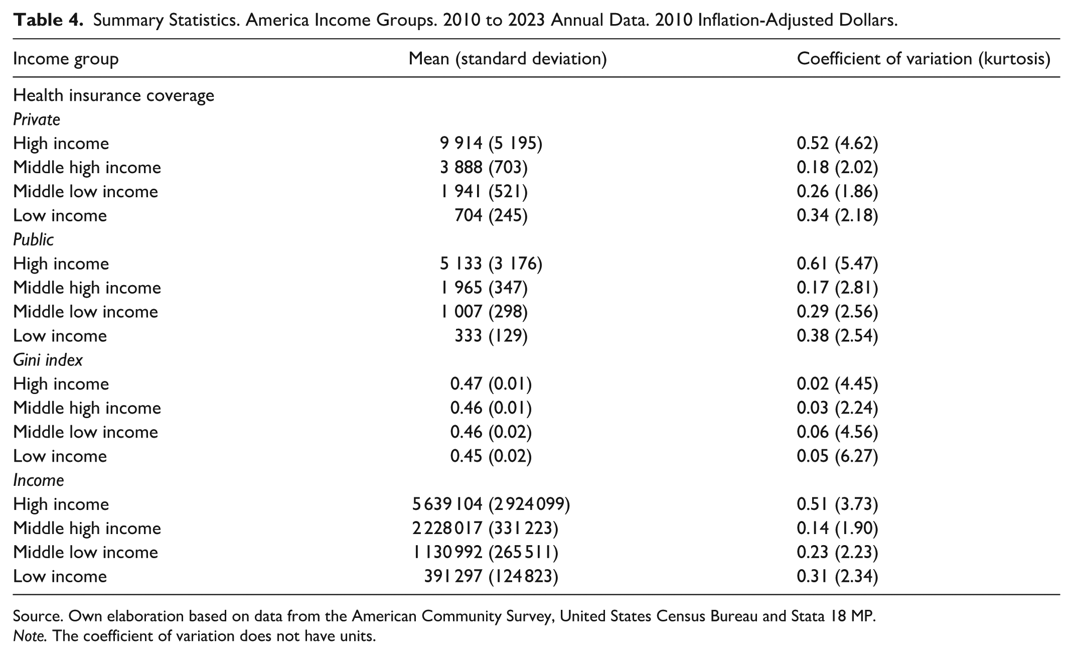
Table 4 reports the summary statistics for each panel model variable. Besides, Table 4 also displays these statistics by income group. The dependent variable is health insurance coverage in its private and public types, which are measured in thousands of people. The independent variables like the Gini index, and income are in 2010 inflation-adjusted United States dollars. Is important to mention that the Gini index of income inequality does not have units. The statistics reported are the mean, standard deviation, coefficient of variation, and kurtosis. The analysis covers 14 years of annual data (2010-2023). The summary statistics describe the shape of the data probability distributions. The mean is computed by adding the annual amounts of each indicator and dividing this total by the number of years under study. The standard deviation is a measure of data dispersion with respect to the mean. As the standard deviation is influenced by the measurement units, it makes difficult its comparison with other variables. The coefficient of variation is obtained by dividing the standard deviation by its mean, providing a measure of data dispersion without units. This lack of units makes easier the data dispersion comparison among different variables. The kurtosis is a statistical measure of the shape of the probability distribution: leptokurtic with low positive values, and platykurtic with high positive values. The kurtosis provides information about the shape of the data distributions, regarding their peakedness around the mean.
Summary Statistics. America Income Groups. 2010 to 2023 Annual Data. 2010 Inflation-Adjusted Dollars.
Source. Own elaboration based on data from the American Community Survey, United States Census Bureau and Stata 18 MP.
Note. The coefficient of variation does not have units.
As shown in Table 4, private health insurance covers more individuals than its public counterpart across all income groups, as evidenced by its mean. The coefficient of variation is larger for public insurance coverage (except in the middle high income group), indicating greater variability in health insurance enrollment. This pattern is corroborated by the kurtosis statistics, as their private values are less than those of their public counterparts. This finding suggests that the private insurance dynamics are more stable.
Increasing insurance enrollment could signal progress toward health equity. Private coverage displays this trend.30,31 The presence of uninsured individuals is attributed to affordability barriers, disproportionately affecting racial and ethnic minorities, immigrants, and less-educated groups. 32 Although, health insurance alone would neither eliminate disparities in access to health care nor equalize health across subgroups on American income groups, a continuous health insurance coverage could improve health outcomes, income stability, and longevity. 33
The Gini index mean indicates that the high income group experiences the greatest income inequality, while low income geographical units report the least inequality. This pattern may reflect the redistributive effects of public welfare programs in low income geographical units, which could help mitigate income disparities. Additionally, the standard deviation, coefficient of variation and kurtosis show similar magnitudes across all the four income groups, suggesting comparable levels of variability in income inequality trends.
The income variable shows significant disparities between high and low income geographical units during the 2010 to 2023 period. For instance, the mean income in the first quartile geographical units is $5 639 104, which is 14.41 times greater than that of low income households. This gap is further emphasized by several measures of variability: a coefficient of variation of 0.51 for high income geographical units, indicating greater income dispersion compared to low income geographical units. This is also indicated by their corresponding kurtosis. Among the remaining groups, the middle low income group exhibited the next highest level of income dispersion.
Method
Panel Model
In what follows the econometric panel model is represented by the following two equations:
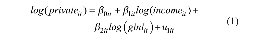

where
Hypothesis
Baseline model hypothesis


where
Fixed effects model hypothesis


The null hypothesis assumes that there is no change in the intercept across income groups. By contrast, the alternative hypothesis allows the intercept to vary across these groups. The time dimension was held constant for both hypotheses. Although, this dimension does not change within income groups, the variation over time is considered between each group. Consequently, the time subscript
Random effects model hypothesis


The null hypothesis assumes the homogeneity of the slopes estimators across income groups. In contrast, the alternative hypothesis allows the slopes for each independent variable (
Results
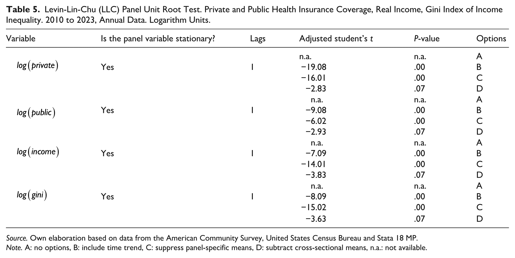
Panel stationarity tests are important because it ensures that the estimated regressions are not spurious. To assess stationarity in panel variables, the Levin-Lin-Chu (LLC) unit root test was used.
All the unit root tests presented in Table 5 indicate that the panel variables are stationary. The LLC test was conducted by using one lag on the logarithms of the variables. The null hypotheses of the test is that the panel contains a unit root, while the alternative hypothesis suggests stationarity. For all the panel variables, the test results indicate stationarity at the 1% significance level. Therefore, the null hypothesis of this test is rejected for all the variables, confirming that the panel variables are stationary.
Levin-Lin-Chu (LLC) Panel Unit Root Test. Private and Public Health Insurance Coverage, Real Income, Gini Index of Income Inequality. 2010 to 2023, Annual Data. Logarithm Units.
Source. Own elaboration based on data from the American Community Survey, United States Census Bureau and Stata 18 MP.
Note. A: no options, B: include time trend, C: suppress panel-specific means, D: subtract cross-sectional means, n.a.: not available.
Equation (1) is estimated using three specifications of the panel model: (i) baseline model, (ii) fixed effects model, and (iii) random effects model. Table 6 reports the estimator coefficients values as elasticities, which measure the percentage change in the dependent variable resulting from a 1% change in the independent variable. The first column presents the elasticities from the baseline model, the second column reports the elasticities from the fixed effects model, and the third column displays elasticities from the random effects model. All estimations were conducted using Ordinary Least Squares (OLS).
Results of the Estimates of Equation (1), 2010 to 2023, Annual Observations. Double Logarithmic Functional Form Log-Log (Student’s t). The Estimators are Elasticities.

Source. Own elaboration based on data from the American Community Survey, United States Census Bureau and Stata 18 MP. The estimator coefficients are read as elasticities because the panel functional form is Log-Log.
Note. All estimators are significant at 99% (***), and n is the number of observations. The number of observations is equal to 13 years times (without accounting for 2020) and 51 geographical units (without accounting for Puerto Rico). The panel model applies dummy variables for each income group: dummy equal to one for income group one and zero for the rest of income groups, dummy equal to one for income group two and zero for the rest of income groups, dummy equal to one for income group three, and zero for the rest of income groups, dummy equal to one for income group four and zero for the rest of income groups, that is, the dummy variable for the income group one is a vector of dimension 1 × 663, with its first 169 rows (13 years times 13 geographical units) equal to one and the rest of 494 rows (13 years times 38 geographical units) equal to zero. The interactions of this dummy for the income group one with the entire data base expresses the intercept or slope estimators for the income group one. Therefore, the number of observations is 663: from these observations 169 belongs to the income group one, the rest of income groups observations 494 becomes zero (13 years times 38 geographical units). 36 The same interactions are applied for each income group, each one of them with its corresponding dummy variable.
From Table 6, the Gini elasticity in the first column is negative (−1.08). This suggests that a 1% increase in the Gini index is associated with a 1.08% decrease in private health insurance coverage across the United States. This effect is further decomposed in the subsequent columns: the fixed effects elasticity in column two yields a value of −1.09, while the random effects elasticities in column three are −1.02, −1.04, −1.90, and −0.67.
In column three, the random effects elasticity for high income states indicates that a 1% increase in the Gini index leads to a 1.02% reduction in private health insurance coverage. For middle high income geographical units, the reduction was 1.04%. The middle low income group experienced the largest decline at −1.90%, while low income geographical units showed a reduction of 0.67%. These results suggest that the middle low income geographical units are the most adversely affected by rising income inequality. This may be because social welfare programs are primarily targeted toward low income geographical units, as suggested by the summary statistics. Consequently, the middle low income group may be relatively disadvantaged. These disparities deserve further analysis, but for the moment it escapes from the scope of this note. Some researches have indicated that disparities in health system performance often reflect broader patterns of social injustice.30,37
In column two, the constant term is examined for each income group using the fixed effects model specification. For the high income group, the initial average level of private health insurance coverage is −7.58 over the 2010 to 2023 period. The middle high and low income groups both show elasticities of −7.60. The low income group reported a slightly higher coefficient of −7.56. These results suggest that, prior to the 2010 to 2023 period, low income geographical units had relatively better private health insurance coverage than the other income groups.
The income estimator reported in the first column of Table 6 is approximately elastic, with a value of 1.01. This suggest that changes in income influence private health insurance coverage in nearly in a one-to-one proportion. To further explore this effect by geographical unit income group, the overall elasticity of 1.01 in column 1 is decomposed into the fixed effects estimator of 1.02 in column two, and random effects estimators of 1.03, 1.03, 0.98, and 1.05, as reported in column three. Overall, these coefficients are almost elastic, suggesting that for a 1% increase in income, private health insurance coverage also increases by 1%. These results suggest a strong and nearly proportional relationship between income and access to private health insurance across all the income groups.
From Table 7 the Gini index estimator in the first column is positive, with a value of 1.56. This indicates that a 1% increase in the Gini index is associated with a 1.56% increase in public health insurance coverage across the United States. This positive relationship suggests that welfare policies respond to rising income inequality by expanding public health insurance coverage across America.
Results of the Estimates of Equation (2), 2010 to 2023, Annual Observations. Double Logarithmic Functional Form Log-Log (Student’s t). The Estimators are Elasticities.

Source. Own elaboration based on data from the American Community Survey, United States Census Bureau and Stata 18 MP. The estimator coefficients are read as elasticities because the econometric panel functional form is Log-Log.
Note. All estimators are significant at 99% (***), and n is the number of observations.
The estimate in column one (1.56) is further decomposed into the fixed effects estimator 1.58 (column two), and the random effects estimators 1.69, 2.69, 2.59, and 0.60 (column three) for high, middle high, middle low, and low income groups, respectively. Specifically, the random effects estimator for high income geographical units suggests that a 1% increase in the Gini index leads to a 1.69% increase in public health insurance coverage. For the middle high income group, the increase is 2.69%, followed by 2.59% for middle low income geographical units, and 0.60% for low income geographical units. These results suggest that middle high income geographical units benefit the most from an increase in income inequality, as public policies, particularly those implemented through social welfare programs, appear to respond more strongly in these geographical units.
Disparities income groups are shown in Table 7. These elasticities are 1.06, 1.12, 1.13, and 1.01, reflecting unequal responses in public health insurance coverage. These figures highlights variations in how geographical units respond to variations in income and income inequality levels on public health insurance programs. Several studies have pointed out that the significant role of income in shaping disparities in health insurance coverage, which, in turn, contributes to differences in health outcomes across regions.21,38 -40
Column two examines the constant term for each income group under the fixed effects model. For high income geographical units, the initial average level of public health insurance coverage (measure over the period 2010-2023) is −6.95, while middle high and low income geographical units report figures of −6.85 and −6.78, respectively. The lowest income geographical unit has a figure of −6.73. These results suggest that, prior to the 2010 to 2023 period, low income geographical units had higher public health insurance coverage than the other income groups.
The income elasticity of public health insurance coverage is close to be unitary, as indicated by the coefficient of 0.99 reported in column one. This elasticity suggests that changes in income influence public health insurance coverage by almost in a one to one proportion. To further examine heterogeneity in the income groups, the overall elasticity in column one (0.99) is decomposed into the fixed effects estimator of 1.07 (column two), and random effects estimators of 1.06, 1.12, 1.13, and 1.01 (column three) for high, middle high, middle low, and low income geographical units, respectively.
Discussion
The summary statistics and panel model results indicate that rising income inequality in the United States exerts opposing effects on health insurance coverage, which negatively affects private health insurance coverage, while positively influencing public health insurance coverage. This suggests that highlighting income inequality at both the national and geographical units’ levels reduce private coverage, but leads to an expansion of public health insurance coverage. Consequently, public policies that do not directly address income inequality may inadvertently increase reliance on public health insurance. As a result, the United State government bears a growing fiscal burden through the expansion of public insurance programs such as Medicaid, Medicare and Veterans Affairs Care to cover the uninsured.
In the corresponding literature health gaps among income groups are underscored by the significant role of public policies in the following areas: (i) health expenditure allocations, (ii) financing and revenue raising mechanisms, (iii) provision and service delivery, (iv) stewardship, (v) monitoring and evaluation, and (vi) cross-sectoral policies outside the health ministry. 41
The results reported in Tables 6 and 7 demonstrate that both private and public health insurance coverage are positively influenced by income increases across American geographical units. It is important to note, that these results are for the period of 2010 to 2023 on average, meaning that they estimates are not specifically applied to a certain year. For brevity, the panel time dimension is not explored in this note. However, in a more extensive research program, a panel time dimension analysis may be feasible.
According to the results in Tables 6 and 7, a 1% increase in income leads to an approximately 1% increase in both private and public health insurance coverage. Conversely, coverage decreases proportionally when income decreases. The structure of the health insurance market, which is defined by the relative composition of private and public coverage, fundamentally depends on the income distribution analyzed in this panel model. This relationship is evident in the income elasticity for private and public insurance. 37 These findings could highlight a concerning cyclical dynamic: constrained healthcare access may perpetuate poverty through financially catastrophic medical expenditures, which in turn exacerbate economic instability and further limit health coverage opportunities. This vicious cycle aligns with the existing literature documenting the bidirectional relationship between socioeconomic status and health outcomes. 42
Observed health insurance disparities across geographical unit income groups (Tables 6 and 7) could reflect social systemic inequalities embedded within the American healthcare model. 37 This model is characterized by high cost and a corporatized structure dominated by private insurance companies. 43 Within this framework, health insurance functions as a commodity driven by market and political priorities rather than the goal of universal coverage. As a result, insurance affordability remains out of reach for vulnerable populations – including low income households, the elderly, and the chronically ill – owing to prohibitive premiums and escalating medical costs. These market failures disproportionally affect individuals lacking employer-sponsored coverage, necessitating large-scale public intervention to absorb the costs of uninsured populations. 43
Empirical analyses employing both time series and cross-section methodologies have found similar results as in this note, regarding the dynamics of health and key economic indicators, corroborating the findings presented in this study.4,44 -48 These consistent results across diverse contexts and methodologies suggest robust underlying mechanisms linking economic conditions to health outcomes.
To enhance both private and public health insurance coverage in the United States, targeted policy interventions aimed at boosting household income – particularly through job creation and wage growth – could provide a sustainable path forward. Expanding health insurance coverage serves as a critical policy to improved population health outcomes, by enabling better access to preventive care, earlier disease detection, and more consistent treatment regimens. 49
Table 2 reports disparities in the Gini index of income inequality by income groups for the period of 2010 to 2023. Associations between income inequality (Gini index) and population health by geographic level using a large, nationally representative dataset of American older adults have found evidence suggesting that income inequality is consistently associated with worse health. This study suggests that further research is necessary to understand the nuances behind these observed associations, which is crucial for designing informed policies and programs that could reduce socioeconomic health inequities among older adults. 50
A study about an income inequality review in the United States has found that government policies and actions since the 1980s played the biggest role in widening the gap between America’s wealthy individuals and everyone else. 51 Other study, points out that the linkages between the distribution of resources within states, the distribution of influence within state political systems, and public policies reflecting distributional decisions, remain largely untested. 52 As long as these nuances briefly outlined in this paragraph are not being studied, the prevailing disparities source of variations could be associated with economic structures, uncoordinated public policy, or demographic factors across geographical units groups. Therefore, we the authors acknowledge that an analysis of conjunctural information can shed light on the determinants that could explain the Gini index paradox depicted in Table 2. Further analysis may be promising in this regard.
The classification of the American geographical units into the four income groups provides information on their respective income levels for the panel model of this note. This income group classification also relates the geographical units to a specific location. A future research vein could consider a regional analysis regarding this geographical dimension, with respect to the Gini index variation. From this regional analysis, contextual results could help in addressing the issue of ecological fallacies. This regional analysis is currently beyond the scope of this note.
The use of the Gini index of income inequality in occasions has been criticized. The same American Community Survey, which produces such an index, recognizes that its computation is not perfectly homogenous for different geographic units: “Users must consider potential differences in geographic boundaries, questionnaire content or coding, or other methodological issues when comparing ACS data from different years. Statistically significant differences shown in ACS Comparison Profiles, or in data users’ own analysis, may be the result of these differences and thus might not necessarily reflect changes to the social, economic, housing, or demographic characteristics being compared.” 53 Given this caveat, the Gini index continues to be the baseline for measuring income inequalities until the moment that a new and more efficient index of income inequality is available. That is why the researcher of these structures must continue relying on the official data of the Gini index of income inequality provided by the ACS, for the time being.
The panel model proposed here has as a goal to build a parsimonious model focused on the primary effects of income and inequality. Including numerous control variables could reduce the degrees of freedom, and potentially introduce bias in the estimators of interest. We recognize this as a limitation of this note.
We acknowledge the potential endogeneity among income, income inequality and health coverage. While Ordinary Least Squares provides Best Linear Unbiased Estimators under its assumptions, we recognize that unobserved factors could simultaneously affect both our independent and dependent variables. Addressing endogeneity with instrumental variables or other advanced methods is a complex task that falls outside the scope of our current analysis. Future research could build on our findings by employing methods designed to address this issue.
Conclusions
The health market structure is assessed through private and public health insurance coverage and analyzed using a panel model for the United States and its 52 geographical units over the period 2010 to 2023. Disparities among geographical units income groups were examined by decomposing national trends with a panel model specification incorporating both fixed and random effects at the income group level.
Overall each of the income group reflects the national pattern observed in the United States, but exhibits distinct elasticity magnitudes. The baseline national estimators (baseline model) are reported in the first columns of Tables 6 and 7, respectively. The fixed effects for individuals at the level of income groups are presented in the second columns, whereas the random effects for individuals at the level of income groups are presented in the third columns of both tables.
Table 3 reports private and public health insurance coverage. It highlights how health system relies on private markets, representing in this way a significant barrier to achieving universal health coverage. This disparity underscores how income directly determines access to care, perpetuating cycles of poor health and poverty. 54 Private health insurance markets systematically discriminate against high-risk individuals, penalizing those who need coverage most. 55 For their part, public health insurance coverage like Medicaid have stringent eligibility criteria (ie, severe disability or poverty), leaving many low-income families without affordable options.56,57 The consequences are stark: uninsured women in the RAND Health Insurance Experiment has mammography rates half those of insured women (32% vs 62%). 58 This disparity underscores how income directly determines access to care, perpetuating cycles of poor health and poverty. 54
Table 4 reports the summary statistics. They reveal that the high income group exhibits the greatest income inequality among the United States geographical units. Results from this Table show that the high income group experiences the strongest negative responses to increases in the Gini index, with a coefficient of −1.02. Paradoxically, the low income group – which maintains a lower baseline Gini index – shows the weakest negative association (−0.67 coefficient) with rising inequality. This differential effect suggests an inconsistency policy response to growing income inequality in public health insurance provision. It is important to emphasize that public health insurance coverage (including Medicaid, Medicare, and Veterans Affairs Care) is ultimately financed through geographical units by means of tax revenues contributed by all America constituents. This funding mechanism raises important equity considerations given the observed disparities in health insurance coverage responsiveness.
The econometric analysis confirms stationarity across all the variables in the panel model, as validated by the LLC unit root test. The elasticities reported in Tables 6 and 7 reveal two distinct, but interrelated, relationships. First, rising income inequality exhibits opposing effects on insurance markets, depressing private health insurance coverage while simultaneously expanding public coverage. Second, income growth demonstrates near unitary elasticity with insurance coverage, with a 1% increase in income producing an approximately a 1% rise in both private and public health insurance coverage across all four income groups and its corresponding geographical units in the United States.
Supplemental Material
sj-pdf-1-inq-10.1177_00469580251405999 – Supplemental material for Health Insurance Coverage and Income Inequality in the United States: Findings from the American Community Survey, 2010 to 2023
Supplemental material, sj-pdf-1-inq-10.1177_00469580251405999 for Health Insurance Coverage and Income Inequality in the United States: Findings from the American Community Survey, 2010 to 2023 by Raúl Enrique Molina-Salazar and Carolina Carbajal-De-Nova in INQUIRY: The Journal of Health Care Organization, Provision, and Financing
Supplemental Material
sj-xlsx-2-inq-10.1177_00469580251405999 – Supplemental material for Health Insurance Coverage and Income Inequality in the United States: Findings from the American Community Survey, 2010 to 2023
Supplemental material, sj-xlsx-2-inq-10.1177_00469580251405999 for Health Insurance Coverage and Income Inequality in the United States: Findings from the American Community Survey, 2010 to 2023 by Raúl Enrique Molina-Salazar and Carolina Carbajal-De-Nova in INQUIRY: The Journal of Health Care Organization, Provision, and Financing
Footnotes
Acknowledgements
We are very grateful to two anonymous referees and numerous colleagues for their useful comments and suggestions.
Ethical Considerations
Not applicable. This paper is desk research. No experiments were performed on humans, or animals, and it did not need ethical approval.
Consent to Participate
Not applicable. No human participation was required for this research.
Consent for Publication
Not applicable. No human consent for publication was required for this research.
Author Contributions
This note contributes to the literature through the novel application of panel models to analyze the relationship among insurance coverage, income and income inequality. The analysis utilizes fixed and random effects models to examine both private and public health insurance coverage across 52 United States geographical units during 2010-2023. This analysis demonstrates how income and income inequality shape insurance coverage.
A parametric analysis demonstrates the divergent effects of income inequality on health insurance across United States geographical units. Income inequality is found to reduce private health insurance coverage (with elasticities ranging from −1.08 to −0.67), while simultaneously increasing public health insurance coverage (with elasticities ranging from +0.60 to +1.58).
This note presents a United States-based analysis of the relationship among insurance coverage, income, and income inequality, using 52 geographical units.
Paradoxical disparities exists in the United States between income levels and access to insurance coverage.
Funding
The authors received no financial support for the research, authorship, and/or publication of this article.
Declaration of Conflicting Interests
The authors declared no potential conflicts of interest with respect to the research, authorship, and/or publication of this article.
Data Availability Statement
The official data for this analysis are sourced from the American Community Survey, conducted by the United States Census Bureau. It is available free of charge on the Bureau’s website.
Supplemental Material
Supplemental material for this article is available online.
References
Supplementary Material
Please find the following supplemental material available below.
For Open Access articles published under a Creative Commons License, all supplemental material carries the same license as the article it is associated with.
For non-Open Access articles published, all supplemental material carries a non-exclusive license, and permission requests for re-use of supplemental material or any part of supplemental material shall be sent directly to the copyright owner as specified in the copyright notice associated with the article.