Sage Journals: Discover world-class research

Abstract

The slowed growth in national health care spending over the past decade has led analysts to question the extent to which this recent slowdown can be explained by predictable factors such as the Great Recession or must be driven by some unpredictable structural change in the health care sector. To help address this question, we first estimate a regression model for state personal health care spending for 1991-2009, with an emphasis on the explanatory power of income, insurance, and provider market characteristics. We then use the results from this simple predictive model to produce state-level projections of health care spending for 2010-2013 to subsequently compare those average projected state values with actual national spending for 2010-2013, finding that at least 70% of the recent slowdown in health care spending can likely be explained by long-standing patterns. We also use the results from this predictive model to both examine the Great Recession’s likely reduction in health care spending and project the Affordable Care Act’s insurance expansion’s likely increase in health care spending.

Keywords

health care spending health insurance health care providers health policy health economics

Background

The growth in national health care spending has slowed considerably over the past several years. For instance, the average annual inflation-adjusted growth rate for national health care spending per capita was 3.76% for years 2000-2007 versus a much lower 1.48% for years 2008-2013.¹ The relatively partisan passage of the 2010 Affordable Care Act (ACA) has made quantifying the determinants of health care spending growth quite politically controversial in recent years. For instance, advocates behind the passage of the ACA tend to credit structural changes to the delivery of health care as a main determinant for the recent reduction in health care spending,² whereas others tend to suggest that the Great Recession was instead responsible for most of this recent reduction in health care spending growth.³

What does the broader literature say about the macro-level determinants of health care spending? Health economists have long agreed that the introduction of new medical technologies over time explains the consistently higher rates of inflation for health care spending compared with the rest of the economy, though other factors explaining rising health care spending include rising real income, increasing insurance, and aging of the population.⁴ More recent analysis has focused on condition-related increases in health care spending, with some analyses of the increases in the prevalence of disease and other analyses of the condition-specific increases in spending per case.^5-7

Regarding the more recent slowdown in health care spending first seen in the late 2000s, some broad analysis focuses on the effect of decreases in real income and their associated changes with individuals moving from private insurance coverage to public insurance coverage or uninsurance.⁸ Moreover, other analysis suggests that a temporary decline in the adoption of expensive new medical technologies explains some of the recent slowdown (along with the rise in high-deductible plans and Medicaid payment reductions) but that prior high growth rates will likely persist due to a sustained pipeline of new technologies.⁹ Other recent analysis also suggests that changes in benefit design of employment-based coverage have had an effect on the recent slowdown in health care spending.¹⁰

Overview of Our Analyses

Our contribution to this literature examining recent changes in health care spending growth is that we not only apply a more systematic approach to modeling long-term health care spending but also exploit the wide geographic variation in total health care spending; see, for instance, the research associated with the Dartmouth Atlas examining geographic variation in Medicare spending.¹¹ Specifically, we focus on the association of health care spending with income, insurance coverage, and provider market characteristics, in which we use a regression-based modeling approach with a relatively longtime series of data, somewhat similar to that used in the modeling of national health care spending.^12-14 However, unlike those long-term models that focus on national health care spending, we build on the Center for Medicare and Medicaid Services (CMS) Office of the Actuary’s separate analysis of state personal health care expenditures.¹⁵ Specifically, we use data for state total health care spending for 1991-2009, available from the National Health Expenditure Accounts (NHEA) data from the CMS Office of the Actuary (as 2009 was the last year these state-level measures were released) and state-level data for various explanatory characteristics.

We then examine the extent to which the recent slowdown in health care spending growth since 2009 can be explained by changes in these characteristics in our state-level model for health care spending. To do so, we first take these models explaining historical state health care spending (with one model for the full 1991-2009 period and a secondary model for just the 2000-2009 period) to make state-level projections of health care spending for 2010-2013. We then compare their amounts, aggregated from the state level to the national level, with actual national health care spending from the CMS NHEA for 2010-2013 to, in turn, make inferences about the extent to which these three sets of explanatory characteristics for income, insurance, and provider markets explain recent spending growth during this 2010-2013 time period.

We also produce estimates of both the likely decrease in health care spending due to the Great Recession’s decline in income and the likely increases in health care spending induced by the ACA’s insurance expansions. For the latter, we apply our observed relationships between insurance and spending from our model (presented below) to the Congressional Budget Office’s (CBO) long-run projected changes in health insurance coverage to determine the likely percent increase in future health care spending induced by the ACA’s insurance expansions. Although the CMS Office of the Actuary projects health care spending to increase in the future due to the improving economy and expanded insurance coverage,^16,17 with the latter due to the strong connection between insurance coverage and health care spending, it does not isolate the independent effects of these factors.

Methodology

To examine these various issues, we first quantify the historical relationship between income, insurance coverage, and provider market dynamics and the magnitude of personal health care spending. Our goal here is not to derive a careful causal effect of any given characteristic on health care spending in isolation. Instead, our goal is to pull together as much comprehensive data as possible (consistent with known causal predictors of health care spending) to include in one single relatively straightforward regression model for total personal health care spending.

Specifically, we estimate a state-level autoregressive model with health care spending as the dependent variable and state-level measures of income, insurance coverage, and provider market characteristics and state fixed effects as the explanatory variables for years 1991-2009. Our analysis uses the 48 contiguous states, as data for some explanatory variables are incomplete for Alaska, Hawaii, and the District of Columbia. Specifically, we estimate a regression model incorporating first-order autocorrelation assumed to have the following form:

Log {HC}_{i t} = α + β {Inc}_{i t} + γ {Ins}_{i t} + δ {Prov}_{i t} + ζ {State}_{i} + v_{i t},

v_{i t} = ε_{i t} - φ v_{i, t - 1} and ε_{i t} ~ N (0, σ^{2}),

where Log HC_it is the log of real total personal health care spending per capita for state i in year t, Inc_it is a set of income measures for state i in year t, Ins_it is a set of health insurance coverage measures for state i in year t, Prov_it is a set of provider market measures for state i in year t, and State_i is an indicator variable for state i. Because the model incorporates an autoregressive process for Log HCit, we do not need to add a time trend variable, particularly because the model’s predicted values of health care spending for 2010-2013 could be sensitive to the choice of the functional form chosen; moreover, a full set of year-by-year indicators is not feasible for generating out-of-sample predictions.

The Yule-Walker estimation method for this autoregressive model is a two-step process in which a naïve ordinary least squares (OLS) model’s residuals (from Equation 1 alone) first generate an initial estimate of the autoregressive parameter, ϕ, which, in turn, generates a variance matrix for v (as specified in Equation 2). This covariance matrix for v then enables a generalized least squares estimation for coefficients β, γ, and δ (from Equation 2).¹⁸ Because our empirical strategy still incorporates repeated observations over time within each state, we generate robust standard errors that account for this clustering.

By examining the log of health care spending per capita as the dependent variable, each of the regression coefficients can be interpreted as the percent change in spending associated with a one-unit change in the explanatory variable. The vector of β coefficients measure the association of health care spending with income, the vector of γ coefficients measure the association with health insurance coverage, and the vector of δ coefficients measure the association with the provider market characteristics.

The remainder of this section provides details about each of these different explanatory measures in this regression model. Partly due to data availability (as indicated below) and partly due to an interest in exploring how the effect of these characteristics might differ over time, we examine regression models for two different time periods: 1991-2009 and 2000-2009. The “Results for the Characteristics Associated With State Health Care Spending” section presents the results for the explanatory effects of these three sets of measures on health care spending from these models.

Data for State Health Care Spending

The data for state personal health care spending, HC_it in the regression equation above, come from the CMS Office of the Actuary’s National Health Expenditures Account data series “National Health Expenditures Accounts by State of Residence” (hereafter referred to as “NHEA-S” to contrast with “NHEA-H” for the subsequent “historical” data series for nationwide spending). These state-level data are for total health care spending, regardless of payer, that is, they are the sum of Medicare spending, Medicaid spending, private insurer spending, and out-of-pocket spending (whether insured or uninsured). However, the state-level data do not include data for “Government Administration and Net Cost of Health Insurance” nor “Government Public Health Activities.” The NHEA-S data are provided by CMS in nominal amounts, but we adjust them (and relevant explanatory variables presented below) for inflation using the Consumer Price Index for All Urban Consumers (CPI-U) by presenting all values in 2014 US dollars.

Data for Explanatory Variables

Income

The first set of explanatory variables, Inc_it, is a set of three state income characteristics. One is the state’s real per capita income in thousands of dollars. These data are available from the Bureau of Economic Analysis’ Regional Economic Accounts (BEA REA) and, like the CMS NHEA-S data, are presented in 2014 dollars here by adjusting by the CPI-U. The second characteristic is the percent of the state population living below the federal poverty line. These data are available from the Census Bureau’s Small Area Income and Poverty Estimates (SAIPE). Values for 1991, 1992, and 1994, which were not produced by the Census, are thus imputed via interpolation using the 1989 (as 1990 is also missing), 1993, and 1995 SAIPE data (and assuming a linear trend by year). The third characteristic is the state unemployment rate. These data are available from the Bureau of Labor Statistics Local Area Unemployment (BLS LAU) data. The rationale here is the literature demonstrating that people generally get healthier in recessions,¹⁹ though the relationship with spending is not obvious, as it is possible that higher health spending (from increased free time) improves health or that improved health decreases health care spending.

Insurance

The second set of explanatory variables, Insit, is a set of insurance coverage measures from the March Supplement of the Current Population Survey (CPS). Specifically, we produce estimates of the percent of the state covered by Medicare or TRICARE, covered by Medicaid or the Children’s Health Insurance Program (CHIP), and covered by private insurance (with the remainder uninsured) The main underlying rationale here (when controlling for income’s effect on affordability) is the “moral hazard” effect of increased consumption of health care when covered by insurance.²⁰ A secondary underlying rationale here is the differences in prices paid for private versus public insurance, Medicare versus Medicaid public insurance, and insurance versus uninsurance. TRICARE is the program covering the military and their dependents (previously known as the Civilian Health and Medical Program of the Uniformed Services, or CHAMPUS), and we pool those covered by TRICARE with those covered by Medicare due to limited sample size of the former, especially for small states in the CPS. Similarly, we do not distinguish employment-based coverage from individual (or “nongroup”) coverage in the privately insured category due to small sample sizes.

We also include a measure of Health Maintenance Organization (HMO) penetration, as HMOs are generally associated with lower health care spending.²¹ Data for 1991-1999 are from Doug Wholey,²² and data for 2002-2012 are from Decision Resources Group’s HealthLeaders/InterStudy (HLIS) survey. To have a consistent measure across the entire period, we define HMO penetration as total enrollment in Medicare Part C (ie, Medicare Advantage after 2003), Medicaid HMOs, and private/commercial HMOs divided by the entire population. After producing analogous data from the 2002-2012 HLIS, we interpolated values for 2000-2001 and extrapolated values for 2013 (assuming a linear trend over time), and divided the total HMO enrollment by the total population.

We also include a measure of self-reported health, partly because those with higher expected spending may be more inclined to obtain health insurance coverage,²³ and therefore there might otherwise be an omitted variable bias for the association of insurance coverage with health care spending. That said, we are also primarily interested in the direct effect of health status on health care spending. Our measure of health status comes from the Behavioral Risk Factor Surveillance System (BRFSS) question, “Would you say that in general your health is excellent, very good, good, fair, or poor?” where we use a measure of the percent of adults reporting fair or poor health. Because this question was added to the BRFSS in 1993 and a few states are missing for certain years (specifically, Wyoming in 1993 and Rhode Island in 1994, whereas District of Columbia missing in 1995 and Hawaii missing in 2004 are not an issue because we only use the 48 contiguous states in our analysis), we extrapolate values for 1991-1992 and those two other observations assuming a linear time trend over time. Although we would ideally include additional measures (such as smoking, obesity, and related chronic conditions) if available throughout this entire time period, self-reported health status has been shown to be a quite valid measure for other specific objective measures of health, including mortality.^24,25

Providers

The third set of explanatory variables, Prov_it, is a set of provider market characteristics for physicians and hospitals. One measure for physicians reflects the malpractice claim environment for the state. Specifically, we include an indicator for whether the state has a law in effect to cap noneconomic damages in jury awards and an indicator for whether the state has a law in effect to replace joint and several liability with proportionate share allocation of liability. These data come from University of Texas Law School Professor Ronen Avraham’s Database of State Tort Law Reforms (DSTLR).²⁶ One underlying rationale here is the direct effect of these reforms on malpractice premiums paid by physicians and the resulting impact of these premiums on provider prices, whereas the second underlying rationale here is the indirect effect of legal liability risk on the practice of “defensive medicine.” Prior research has found that caps on noneconomic damages decrease health care spending, whereas joint and several reforms increase health care spending (with the thought that proportionate share allocation seems to actually increase risk of lawsuits for physicians, as plaintiffs formerly focused on targeting hospitals).^27,28

A second measure for physicians is the number of physicians per capita, which reflects the equilibrium for both supply and demand. These county-level data are available from the Health Resources and Services Aministration’s (HRSA) Area Health Resources File (AHRF) for 1990, 1995, and 2000-2013. Values for 1991-1994 and 1996-1999 are imputed as a linear trend from 1990, 1995, and 2000. More physicians per capita could increase spending through welfare improvements in access to care or inefficiencies associated with supplier-induced demand, whereas fewer physicians per capita could alternatively increase spending through decreased price competition.²⁹

One measure for hospitals is the number of general community hospital beds per capita, which also reflects the equilibrium for both supply and demand. These data are constructed from HRSA’s AHRF for 1991-1999 and from the American Hospital Association’s (AHA) Annual Survey for 2000-2013. More hospital beds could likewise increase spending through improved access or increased supplier-induced demand, whereas fewer hospitals could likewise increase hospital prices through increased price competition.³⁰

A second measure for hospitals is a more accurate measure of hospital market concentration for years 2000-2013, again with the rationale that hospitals with increased market power will have higher prices for those with private insurance. (We do not have access to these propriety AHA data before 2000.) Specifically, we first construct a market-level concentration measure based on the commonly used Herfindahl-Hirschman Index (HHI) using Core-Based Statistical Areas, and their Metropolitan Divisions (CBSD) therein, to define geographic markets and hospital market shares using the AHA’s private-pay inpatient days aggregated to the hospital system within the market. For nonmetropolitan areas outside CBSDs, we define the market as the nonmetropolitan collection of counties within the state. We then take the average of the market-level HHI measures across the state, weighting by county population. (We use only private-pay inpatient days rather than all inpatient days, because market concentration in the Medicare and Medicaid markets would not have an effect on Medicare or Medicaid prices.)

We also examine a measure of average insurer market concentration within the state using data available from HLIS for 2005-2009 (as data to construct concentration measures using both Preferred Provider Organization (PPO) and HMO data enrollment are only available from HLIS for 2005 onward). The rationale here is that insurers with increased market power will negotiate lower physician and hospital prices.³¹ (Because the CMS state-level NHEA-S data do not include the “Net Cost of Health Insurance” measures, we would not detect a marginal effect of insurer market concentration on the administrative markup of private premiums.) Similar to our hospital market concentration measure, we construct a market-level HHI defining geographic markets with CBSDs, using private insurer market shares from the HLIS census of private insurers and averaging these market-level measures across the state using county population. Because of the relatively short time period (which limits the ability of our state fixed-effects analyses to detect relationships), and because this measure of insurer market concentration ultimately has an insignificant association with health care spending, we do not show these regression results for the 2005-2009 subsample. Because insurer market concentration is unrelated to fee-for-service Medicare and Medicaid prices, the insignificant result is not unexpected.

Finally, we include a measure of the percent of the state population living in a nonmetropolitan area—specifically, not in either Metropolitan or Micropolitan CBSDs, as defined by the Office of Management and Budget (OMB). These data are available from HRSA’s AHRF.

As noted above, the causal inference of these characteristics on spending from our analysis is limited by the lack of exogenous instruments for the explanatory variables (and thereby subject to possible reverse causality). Although an explanation for higher spending leading to higher income is unclear, high spending could lead to increased insurance coverage through a higher demand for insurance or lead to decreased insurance coverage through reduced affordability. Moreover, high health care spending could lead to increased consumer demand for HMOs, attenuating our expected result. Endogeneity is also a concern for our provider measures, in that high spending could lead to an increase in the supply of physicians and hospitals, thereby likely biasing the supply measures’ relationship upward but biasing the market concentration measure’s relationship downward.

Results for the Characteristics Associated With State Health Care Spending

Table 1 presents the mean values for all of these state-level measures described in the “Methodology” section. As noted above, the unit of observation in this table and in our subsequent regression analyses is the state × year, and the sample includes the 48 contiguous states. The first two columns represent the two time periods we use for our regression analyses (ie, 1991-2009 and 2000-2009), with the latter based on data availability for the hospital market concentration measures and also our interest in seeing whether there are any differences in the association between health care spending and these various characteristics over time. (To that end, we also examine the 2000-2009 models without hospital market concentration to have the same set of explanatory variables.) The final column shows all of these measures (except for state personal health care spending per capita) for 2010-2013, with which we generate predicted values of state spending for 2010-2013 from the 1991-2009 model and the 2000-2009 model.

Table 1.

Summary Statistics for State-Level Personal Health Care Spending and the Explanatory Characteristics.

	Years 1991-2009: sample mean (SD) for Model 1	Years 2000-2009: sample mean (SD) for Model 2	Years 2010-2013: sample mean (SD) for projections
Real all-payer personal health care per capita (2014 US$; Source: CMS)	5998.06 (1355.09)	6853.44 (1138.58)	NA
Real per capita income in thousands (2014 US$; Source: BEA REA)	39.09 (7.28)	42.11 (7.18)	44.20 (8.02)
Percent below the poverty line (Source: Census SAIPE)	12.97 (3.45)	12.59 (3.13)	15.39 (3.14)
Unemployment rate (Source: BLS LAU)	5.38 (1.64)	5.27 (1.67)	7.92 (1.99)
Percent covered by Medicare or TRICARE (Source: CPS)	16.92 (2.68)	17.08 (2.75)	18.83 (2.86)
Percent covered by Medicaid/CHIP (Source: CPS)	9.20 (3.15)	9.96 (3.14)	13.22 (3.39)
Percent covered by private insurance (Source: CPS)	59.41 (6.16)	59.11 (6.20)	53.43 (5.84)
Percent uninsured (Source: CPS)	14.47 (4.11)	13.85 (3.83)	14.52 (4.05)
HMO penetration for Medicare, Medicaid, and private plans (Sources: Wholey and HLIS)	19.23 (11.64)	20.83 (11.90)	19.16 (11.09)
Percent of population reporting fair/poor health (Source: BRFSS)	14.54 (3.51)	15.30 (3.32)	16.90 (3.51)
Malpractice reform (0/1): caps on noneconomic damages (Source: Avraham’s DSTLR)	0.26 (NA)	0.32 (NA)	0.38 (NA)
Malpractice reform (0/1): joint and several liability reform (Source: Avraham’s DSTLR)	0.69 (NA)	0.73 (NA)	0.76 (NA)
Physicians per 10 000 capita (Source: HRSA’s AHRF)	21.84 (7.01)	22.98 (7.04)	24.10 (7.60)
General community hospital beds per 10 000 capita (Sources: HRSA’s AHRF and AHA)	33.21 (12.13)	29.14 (9.83)	26.56 (8.06)
Hospital market concentration’s average CBSD-level HHI across states (thousands; Source: AHA)	NA	39.19 (13.06)	40.76 (12.61)
Percent of population not in metro/micro CBSD (Source: HRSA’s AHRF)	10.95 (10.13)	10.61 (9.82)	10.10 (9.39)
No. of observations	912	480	192

Note. The unit of observation is the state × year for the 48 contiguous states in various subsamples by year. All dollar values are inflation-adjusted to 2014 US$ values using the CPI-U series. NA = Not Applicable; CMS = Center for Medicare and Medicaid Service; BEA REA = Bureau of Economic Analysis’ Regional Economic Account; SAIPE = Small Area Income and Poverty Estimate; BLS LAU = Bureau of Labor Statistics Local Area Unemployment; CPS = Current Population Survey; CHIP = Children’s Health Insurance Program; HMO = Health Maintenance Organization; HLIS = HealthLeaders/InterStudy; BRFSS = Behavioral Risk Factor Surveillance System; DSTLR = Database of State Tort Law Reform; HRSA’s AHRF = Health Resources and Services Administration’s Area Health Resources File; AHA = American Hospital Association; HHI = Herfindahl-Hirschman Index; CPI-U = Consumer Price Index for All Urban Consumer; CBSD = Core-Based Statistical Area with Metropolitan Divisions.

Tables 2 and 3 show the results from our regression analyses to examine the log of inflation-adjusted all-payer state personal health care spending by year. The two columns of Table 2 show the regression coefficients (interpreted as percent changes with respect to one-unit changes in the explanatory characteristic) from the generalized least squares regression for a first-order autocorrelation using the Yule-Walk estimation method, with the model’s results for the years 1991-2009 in the first column and the model’s results for the years 2000-2009 (for which hospital market concentration is available) in the second column. (The coefficients for the state fixed effects are not shown.) The Durbin-Watson statistics are relatively high (ie, 1.04 for the 1991-2009 analysis and 1.90 for the 2000-2009 analysis) suggesting that the first-order autoregressive model is warranted due to serial correlation across years. Table 3 converts these regression coefficients to elasticity estimates for statistically significant values and for relevant measures (ie, not the state tort reform law indicators).

Table 2.

Regression Results for Percent Changes in State-Level Real All-Payer Personal Health Care per Capita.

	Model 1: years 1991-2009	Model 2: years 2000-2009
Intercept for log real all-payer personal health care per capita (2014 US$)	6.55 [3.18]**	8.04 [0.28]***
Real per capita income in thousands (2014 US$; Source: BEA REA)	1.31 [0.08]***	1.46 [0.20]***
Percent below the poverty line (Source: Census SAIPE)	0.61 [0.10]***	1.63 [0.22]***
Unemployment rate (Source: BLS LAU)	0.98 [0.07]***	1.18 [0.15]***
Percent covered by Medicare or TRICARE (Source: CPS)	0.08 [0.05]*	0.20 [0.13]
Percent covered by Medicaid/CHIP (Source: CPS)	0.16 [0.04]***	0.40 [0.13]***
Percent covered by private insurance (Source: CPS)	−0.03 [0.03]	−0.03 [0.09]
Percent uninsured (Source: CPS)	Ref. [NA]	Ref. [NA]
HMO penetration for Medicare, Medicaid, and private plans (Sources: Wholey and HLIS)	−0.04 [0.02]**	−0.14 [0.04]***
Percent of population reporting fair/poor health (Source: BRFSS)	0.01 [0.05]	−0.01 [0.13]
Malpractice reform (0/1): caps on noneconomic damages (Source: Avraham’s DSTLR)	−0.07 [0.38]	1.41 [0.70]**
Malpractice reform (0/1): joint and several liability reform (Source: Avraham’s DSTLR)	1.39 [0.28]***	1.47 [0.77]*
Physicians per 10 000 capita (Source: HRSA’s AHRF)	1.84 [0.19]***	2.32 [0.53]***
General community hospital beds per 10 000 capita (Sources: HRSA’s AHRF and AHA)	−0.32 [0.04]***	−0.60 [0.15]***
Hospital market concentration’s average CBSD-level HHI across State (thousands; Source: AHA)	NA	0.09 [0.09]
Percent of population not in metro/micro CBSD (Source: HRSA’s AHRF)	−5.05 [0.60]***	−2.84 [0.80]***
Durbin-Watson statistic	1.04	1.90
Autoregressive correlation parameter	0.707	0.514
No. of observations	912	480

Note. The unit of observation for these models is the state × year for the 48 contiguous states. The analysis uses a first-order autoregressive model with state fixed effects using the Yule-Walker method for estimating parameter values. The dependent variable is the log of the state’s real (ie, inflation-adjusted to 2014 US$ values using the CPI-U series) all-payer personal health care spending per capita from the National Health Expenditures Accounts data from the CMS Office of the Actuary. The explanatory variables are described in the text. Standard errors for the regression coefficients accounting for state clustering are in brackets. Results for 2000-2009 excluding hospital market concentration (available on request) are similar to the results shown here for 2000-2009 that include it. BEA REA = Bureau of Economic Analysis’ Regional Economic Account; SAIPE = Small Area Income and Poverty Estimate; BLS LAU = Bureau of Labor Statistics Local Area Unemployment; CPS = Current Population Survey; CHIP = Children’s Health Insurance Program; HMO = Health Maintenance Organization; HLIS = HealthLeaders/InterStudy; BRFSS = Behavioral Risk Factor Surveillance System; DSTLR = Database of State Tort Law Reform; HRSA’s AHRF = Health Resources and Services Administration’s Area Health Resources File; AHA = American Hospital Association; HHI = Herfindahl-Hirschman Index; CPI-U = Consumer Price Index for All Urban Consumer; CBSD = Core-Based Statistical Area with Metropolitan Divisions.

P ≤ .10. **P ≤ .05. ***P ≤ .01.

Table 3.

Elasticity Estimates for Changes in All-Payer Personal Health Care per Capita With Respect to Changes in Relevant Characteristics.

	Model 1: years 1991-2009	Model 2: years 2000-2009
Real per capita income	0.51	0.61
Percent below the poverty line	0.08	0.21
Unemployment rate	0.05	0.06
Percent covered by Medicare or TRICARE	0.01	ns
Percent covered by Medicaid/CHIP	0.01	0.04
HMO penetration for Medicare/Medicaid/private plans	−0.01	−0.03
Physicians per capita	0.40	0.53
General community hospital beds per capita	−0.11	−0.17
Percent nonmetropolitan/micropolitan	−1.98	−0.30

Note. Elasticity estimates are derived from the statistically significant results presented in Table 2. ns = not significant. CHIP = Children’s Health Insurance Program; HMO = Health Maintenance Organization.

Regarding the income variables, an increase of real per capita income is, as expected, significantly associated with increases in health care spending in both the 1991-2009 and 2000-2009 models; the elasticity estimates are 0.51 and 0.61, respectively. An increase in the poverty rate is significantly associated with an increase in health care spending in both the 1991-2009 and 2000-2009 models; the elasticity estimates are 0.08 and 0.21, respectively. An increase in the unemployment rate is significantly associated with an increase in health care spending in both the 1991-2009 and 2000-2009 models; the elasticity estimates are 0.05 and 0.06, respectively. (We discuss the implications of these findings for income in more detail below in the “Conclusion” section in the context of the impact of the Great Recession.)

Regarding the insurance characteristics, increases in the percent with insurance coverage (relative to being uninsured) are sometimes significantly associated with increases in health care spending. The percent covered by Medicare or TRICARE has a marginally significant 0.01 elasticity in the 1991-2009 model, but is insignificant in the 2000-2009 model. The percent covered by Medicaid or CHIP has significant 0.01 and 0.04 elasticities in the 1991-2009 and 2000-2009 models, respectively. The percent covered by private insurance is insignificant in both the 1991-2009 and 2000-2009 models. The stronger relationship for Medicaid observed in the 2000-2009 period relative to the 1991-2009 period may result from noise in the earlier years before the so-called “verification question” change to the CPS insurance questions in 2000. (We discuss the implications of these findings in more detail below in the “Conclusion” section in the context of the ACA’s insurance expansions.)

Moreover, the HMO penetration rate is, as expected, significantly associated with decreases in health care spending in both the 1991-2009 and 2000-2009 models; the elasticity estimates are −0.01 and −0.03, respectively. In addition, the percent of the adult population reporting fair or poor health status is not associated with health care spending in either model.

Regarding the provider market characteristics related to physicians, state malpractice reforms to cap noneconomic damages was unexpectedly unrelated to health care spending in the 1991-2009 model and significantly associated with increases in health care spending in the 2000-2009 model. State malpractice reforms to replace joint and several liability with proportionate share allocation of liability was, as expected, significantly associated with increases in health care spending in the 1991-2009 and 2000-2009 models. Moreover, an increase in the number of physicians per capita is, as expected, significantly associated with increases in health care spending in both the 1991-2009 and 2000-2009 models; the elasticity estimates are 0.40 and 0.53, respectively.

Regarding the hospital market characteristics, an increase in the number of hospital beds per capita is significantly associated with a decrease in health care spending in the 1991-2009 and 2000-2009 models; the elasticity estimates are −0.11 and −0.17, respectively. However, an increase in hospital market concentration is not associated with increases in health care spending. As noted above, this finding for hospital market concentration is likely attenuated because hospital market concentration is unrelated to prices paid for Medicare and Medicaid beneficiaries.

Results for the Projections of State Health Care Spending Out to 2013

We next use these regression results from the prior “Results for the Characteristics Associated With State Health Care Spending” section to produce estimates of projected health care spending for years 2010-2013 using the state-level income, insurance, and provider market characteristics for years 2010-2013 as the explanatory variables. Recall that the average values for these explanatory variables during this time period are shown in the final column of Table 1. We compare these projections from the state-based regression model with actual national health care spending subsequently released by CMS in their NHEA-H series below.

Figure 1 presents a graph with these personal health care spending per capita estimates. The top shows the data for the entire 1991-2013 period on the x-axis, whereas the bottom then focuses on the upper right portion in the dotted-line box to better observe the data series from 2005 onward. The first series in blue simply presents the NHEA-H data for the entire 1991-2013 period, where the only change is to make an adjustment for inflation using the CPI-U. The second series in blue simply presents the average NHEA-S data for the 1991-2009 period (using state population by year to compute these weighted averages). Overall, the two data series track each other closely with deviations potentially explained by the NHEA-S data we present omitting Alaska, Hawaii, and District of Columbia and perhaps by subsequent minor revisions to the NHEA-H data series after the 2009 NHEA-S data were finalized (and thus not subsequently revised).

Figure 1.

Comparison of actual spending and counterfactual spending with the 1991-2009 prediction model.

The average predicted values from the 1991-2009 regression model are shown in red in the figure for 1991 through 2013. The state-level regression model using the full 1991-2009 period with the available income, insurance, and provider explanatory variables generates a predicted value of $7963 for real per capita health care spending in 2013 (in inflation-adjusted 2014 US$). The state-level regression model using the 2000-2009 period with these explanatory variables along with hospital market concentration generates a slightly higher predicted value of $8150 for real per capita health care spending in 2013 (in 2014 US$) and is not included in the figure. These estimates for 2013 (and additional ones described below) are shown in Table 4.

Table 4.

Decomposing the Likely Causes of the Recent Slowdown in Health Care Spending Growth.

	Results from Model 1: years 1991-2009	Results from Model 2: years 2000-2009
Counterfactual national personal health care per capita (2014 US$), from trending at a 3% real growth rate	$8566	$8696
Actual national personal health care per capita (2014 US$), from the CMS NHEA-H series	$7953	$7953
Average predicted state personal health care per capita (2014 US$), from the model specified here	$7963	$8150
Average predicted state personal health care per capita (2014 US$), from the model specified here, but assuming there was no recession	$8215	$8461
Percent of the difference between counterfactual and actual spending explained by known characteristics in the model specified here	98%	73%
Percent of the difference between counterfactual and actual spending explained by recession’s decline in real per capita income	41%	42%
Percent of the difference between counterfactual and actual spending explained by other known characteristics in the model	57%	32%
Percent of the difference between counterfactual and actual spending unexplained by the model specified here	2%	27%

Note. The methods and assumptions for determining these dollar estimates for counterfactual, actual, and average predicted health care spending are provided in the text. Similarly, the methods and assumptions for determining the percent of the difference between counterfactual and actual spending explained by the recession, other known characteristics in the model, and the unexplained residual are also provided in the text. CMS = Center for Medicare and Medicaid Service; NHEA-H = National Health Expenditure Accounts - Historical.

While actual real per capita health care spending from the CMS NHEA-H data was $7953 (in 2014 US$), what would 2013 health care spending have been in the absence of the recent slowdown in the growth rate? One counterfactual (shown in green in Figure 1) is that the 2009 value for real national health care spending per capita of $7624 (in 2014 US$) could have grown at a real rate of 3.0%, equal to the average 1991-2009 real growth rate from $4521 in 1999 (in 2014 US$). Under this scenario, 2013’s health care spending per capita (in 2014 US$) would have instead been $8566 (as shown in the first row of Table 4). As a result, $603 (ie, $8566 − $7963, where $7963 is the 1991-2009 model’s prediction for 2013) of the naïve $613 decline (ie, $8566 − $7953, where $7953 is the actual 2013 amount) can be explained by changes in these predictable income, insurance, and provider characteristics. In other words, fully 98% (ie, $603/$613) of the recent slowdown in health care spending can perhaps be explained by the predictable characteristics rather than structural changes to the health care sector. Similarly, using the 2000-2009 model’s projection of $8150 for 2013 spending (in 2014 US$) compared with a counterfactual $8696 for 2013 spending (in 2014 US$) from applying the 3.3% real growth rate observed for 2000-2009 implies that 73% of the recent slowdown that can be explained by predictable factors.) Graphically, almost all of 2013’s difference between the blue and green lines can be explained by the difference between the red and green lines. This finding is dependent on the assumption made above about the unobserved counterfactual growth rate in spending if the recent slowdown in spending had not actually occurred. If a higher (or lower) trend were assumed, the percentage spending reduction explained by the model would decrease (or increase).

We also explore the extent to which the Great Recession versus other known characteristics appears responsible for the recent decline in health care spending. To do so, we produce a counterfactual level of per capita income in 2013 as if the Great Recession had not occurred, and determine the level of predicted health care spending at that higher level of income. (We essentially assume that the poverty rate and unemployment rate returned to “natural” levels by 2013, but the recession caused a sustained decline in income.) Specifically, we estimate that real per capita income in 2013 would have been $48 200 instead of $45 400 (from continuing the observed 2000-2006 trend of a 1.1% real annual growth rate in per capita income for 2007-2013 instead of the actual 0.2% real annual growth rate observed). Based on the 0.51 income elasticity observed in the 1991-2009 model, this generates an estimate of $8215 for expected health care spending in the absence of the Great Recession (as shown in Table 4), which then suggests that the likely permanent decline in real per capita income is responsible for 41% of the slowdown in health care spending, that is, ($8215 − $7963) / ($8566 − $7953). This, in turn, implies that the other known characteristics in the model combined to explain 57% of the predictable decline (to sum up to 98%). A similar exercise using the 2000-2009 model’s results suggest that 42% of the slowed growth can be explained by the Great Recession, whereas 32% of the slowed growth can be explained by other known characteristics (to sum up to 73%).

Finally, we use the regression results from the “Results for the Characteristics Associated With State Health Care Spending” section to produce estimates of the likely increases in personal health care spending associated with the ACA’s Medicaid expansions. To do so, we rely on projections of the ACA’s likely changes in health insurance coverage from the Congressional Budget Office (CBO), supplemented with insurance coverage data for Medicare and TRICARE from the Current Population Survey. The first column of the top panel of Table 5 shows CBO’s recent estimates of insurance coverage in 2019 if the ACA were not in effect, whereas the second column of Table 5’s top panel shows CBO’s estimates of insurance coverage in 2019 with the ACA in effect.³² For instance, CBO estimates that after the ACA is fully implemented, those who are uninsured will decrease from 14.7% of the US population to 7.8% of the population, and that those covered by Medicaid/CHIP will increase from 12.0% of the population to 15.6% of the population.

Table 5.

Expected Relationship of the ACA’s Insurance Expansions With Future Health Care Spending.

	2019 coverage, without ACA (%)	2019 coverage, with ACA (%)
Medicare’s coverage	17.7	17.7
TRICARE coverage	2.9	2.9
Medicaid/CHIP’s coverage	12.0	15.6
Employer’s coverage	47.6	45.2
Individual’s coverage	5.2	4.0
Exchanges’ coverage	0.0	6.9
Uninsured	14.7	7.8
Medicaid/CHIP’s change in spending		0.6-1.4 (average = 1.0%)

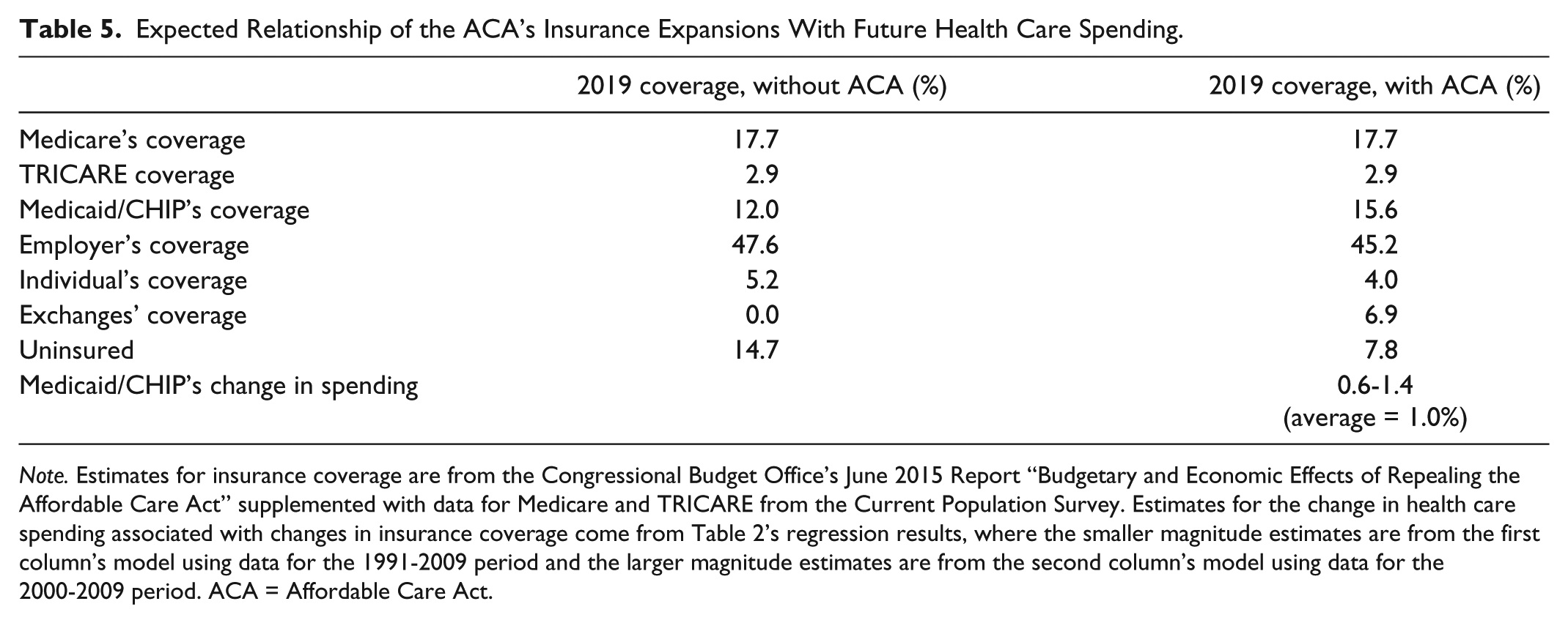
Note. Estimates for insurance coverage are from the Congressional Budget Office’s June 2015 Report “Budgetary and Economic Effects of Repealing the Affordable Care Act” supplemented with data for Medicare and TRICARE from the Current Population Survey. Estimates for the change in health care spending associated with changes in insurance coverage come from Table 2’s regression results, where the smaller magnitude estimates are from the first column’s model using data for the 1991-2009 period and the larger magnitude estimates are from the second column’s model using data for the 2000-2009 period. ACA = Affordable Care Act.

The bottom panel of Table 5 shows the range in the likely relationship between the Medicaid expansion with total health care spending by applying the results from Table 2’s models for the 1991-2009 and 2000-2009 periods. (Recall that the effect was smaller in magnitude for the 1991-2009 model relative to the 2000-2009 model.) Applying these relationships for Medicaid/CHIP coverage to these CBO projections for changes in insurance coverage generate these estimates of the partial change in health care spending. Applying the 0.40 coefficient for Medicaid/CHIP coverage in 2000-2009 to the 3.6 percentage point increase in Medicaid/CHIP coverage gives the upper range estimate of a 1.4% increase in health care spending, whereas applying the 0.16 coefficient gives the lower range estimate of 0.6%. That is, the level of spending in 2019 is expected to be, averaging these two estimates, about 1.0% higher with the ACA’s Medicaid expansions than it would be without the ACA’s Medicaid expansions. Practically, because CBO anticipates that insurance expansions will gradually increase coverage from 2014 to 2019, this 1.0% increase would be seen in slightly higher annual growth rates for health care spending during the 2014-2019 period.

Conclusion

Using data from the CMS NHEA-S data series for 1991-2009, we find that a number of state-level characteristics are significantly associated with state personal health care spending. These include real income, the percent in poverty, the percent insured by Medicaid, HMO penetration, malpractice reform to joint and several rules, the number of physicians and hospitals, and the percent of the population residing in nonmetropolitan areas. Our take is that the magnitudes of these estimates are both mostly comparable between the 1991-2009 and 2000-2009 models and generally consistent with the literature (when it exists for a given characteristic).

Although there is value to these estimates, in and of themselves, there are also interesting policy implications from applying these findings to recent and anticipated health care spending. Specifically, when comparing actual and counterfactual spending in 2013 with the projected 2013 spending from our 1991-2009 and 2000-2009 autoregressive models using state-level variation in explanatory income, insurance, and provider characteristics, we find that at least 70%, if not all, of the recent slowdown in health care spending appears to be explained by these predictable factors (although this finding relies on the assumption made about the unobserved growth in counterfactual spending). The most important one of these factors appears to be the Great Recession’s effect on reduced real per capita income and the subsequent effect on reduced health care spending, as about 41% of the recent slowdown can be explained by these reductions in income. Our findings are therefore consistent with other research that finds that the recession’s decline in income is a major influence on health care spending.^3,8 Second, when applying our regression model’s estimates for the relationship between Medicaid coverage and health care spending to the CBO’s projections of changes in Medicaid coverage resulting from the ACA’s insurance expansions, we find that the level of total health care spending in 2019 is likely to be about 1% higher than it would have been in the absence of these expansions.

Footnotes

Authors’ Note

The findings and conclusions in this article are those of the authors and do not necessarily represent the views of the Mercatus Center.

Declaration of Conflicting Interests

The author(s) declared no potential conflicts of interest with respect to the research, authorship, and/or publication of this article.

Funding

The author(s) disclosed receipt of the following financial support for the research, authorship, and/or publication of this article: This research was funded by George Mason University’s Mercatus Center.

References

Hartman

Martin

Lassman

Catlin

; the National Health Expenditure Accounts Team. National health spending in 2013: growth slows, remains in step with the overall economy. Health Aff. 2015;34(1):150-160.

Cutler

Sahni

NR.

If slow rate of health care spending growth persists, projections may be off by $770 billion. Health Aff. 2013;32(5):841-850.

Dranove

Garthwaite

Ody

Health spending slowdown is mostly due to economic factors, not structural change in the health care sector. Health Aff. 2014;33(8):1399-1406.

Newhouse

JP.

Medical care costs: how much welfare loss?

J Econ Perspect. 1992;6(3):3-21.

Roehrig

Rousseau

DM.

The growth in cost per case explains far more of us health spending increases than rising disease prevalence. Health Aff. 2011;30(9):1657-1663.

Thorpe

KE.

Treated disease prevalence and spending per treated case drove most of the growth in health care spending in 1987-2009. Health Aff. 2013;32(5):851-858.

Starr

Dominiak

Aizcorbe

Decomposing growth in spending finds annual cost of treatment contributed most to spending growth, 1980-2006. Health Aff. 2014;33(5):823-831.

Holohan

McMorrow

What drove the recent slowdown in health spending growth and can it continue?

Urban Institute Report, Washington, DC. http://www.urban.org/research/publication/what-drove-recent-slowdown-health-spending-growth-and-can-it-continue/view/full_report. Published May 6, 2013.

Chandra

Holmes

Skinner

Is this time different? The slowdown in healthcare spending. NBER (Working Paper No. 19700), Boston, MA. http://www.nber.org/papers/w19700. Published December 2013.

10.

Ryu

Gibson

McKellar

Chernew

ME.

The slowdown in health care spending in 2009–11 reflected factors other than the weak economy and thus may persist. Health Aff. 2013;32(5):835-840.

11.

Fisher

Goodman

Skinner

Bronner

Tracking the Care of Patients With Severe Chronic Illness: The Dartmouth Atlas of Health Care 2008. Hanover, Germany: The Dartmouth Institute for Health Policy and Clinical Practice; 2008.

12.

Getzen

TE.

Forecasting health expenditures: short, medium and long (long) term. J Health Care Finance. 2000;26:56-72.

13.

CMS Office of the Actuary. Projections of National Health Expenditures: Methodology and Model Specification, Baltimore, MD. https://www.cms.gov/Research-Statistics-Data-and-Systems/Statistics-Trends-and-Reports/NationalHealthExpendData/downloads/projections-methodology.PDF. Published July 28, 2011.

14.

Kaiser Family Foundation and Altarum Institute. Assessing the Effects of the Economy on the Recent Slowdown in Health Spending. Kaiser Family Foundation and Altarum Institute Report, Menlo Park, CA. http://kff.org/health-costs/issuebrief/assessing-the-effects-of-the-economy-on-the-recentslowdown-in-health-spending-2/. Published April 22, 2013.

15.

Cuckler

Sisko

AM.

Modeling per capita state health expenditure variation: state-level characteristics matter. Medicare & Medicaid Research Review. 2013;3(4):1-21.

16.

Sisko

Keehan

Cuckler

. National health expenditure projections, 2013–23: faster growth expected with expanded coverage and improving economy. Health Aff. 2014;33(10):1841-1850.

17.

Keehan

Cuckler

Sisko

. National health expenditure projections, 2014–24: spending growth faster than recent trends. Health Aff. 2015;34(8):1407-1417.

18.

Gallant

Goebel

JJ.

Nonlinear regression with autoregressive errors. J Am Stat Assoc. 1976;71:961-967.

19.

Ruhm

CJ.

Are recessions good for your health?

Q J Econ. 2000;115(2):617-650.

20.

Pauly

MV.

The economics of moral hazard: comment. Am Econ Rev. 1968;58(3):531-537.

21.

Manning

Leibowitz

Goldberg

Rogers

Newhouse

JP.

A controlled trial of the effect of a prepaid group practice on use of services. N Engl J Med. 1984;310(23):1505-1510.

22.

Wholey

Christianson

Engberg

Bryce

HMO market structure and performance, 1985 to 1995. Health Aff. 1997;16(6):75-84.

23.

Bundorf

Herring

Pauly

Health risk, income, and the purchase of private health insurance. Forum Health Econ Pol. 2010;13(2):1-33.

24.

Idler

Benyamini

Self-rated health and mortality: a review of twenty-seven community studies. J Health Soc Behav. 1997;38(1):21-37.

25.

Franks

Gold

Fiscella

Sociodemographics, self-rated health, and mortality in the US. Soc Sci Med. 2003;56:2505-2514.

26.

Dafny

Avraham

Schanzenbach

The impact of tort reform on employer-sponsored health insurance premiums. J Law Econ Organ. 2012;28(4):657-686.

27.

Kessler

McClellan

Do doctors practice defensive medicine?

Q J Econ. 1996;11:353-390.

28.

Congressional Budget Office. Medical Malpractice Tort Limits and Health Care Spending, Washington, DC. https://www.cbo.gov/publication/17748. Published April 1, 2006.

29.

Cromwell

Mitchell

Physician-induced demand for surgery. J Health Econ. 1986;5(4):293-313.

30.

Gaynor

Town

Competition in health care markets. In: Pauly

McGuire

Barros

, eds. Handbook of health economics. Vol. 2. Amsterdam, The Netherlands: Elsevier; 2011:499-637.

31.

Trish

Herring

How do health insurer market concentration and bargaining power with hospitals affect health insurance premiums?

J Health Econ. 2015;42:104-114.

32.

Congressional Budget Office. Budgetary and Economic Effects of Repealing the Affordable Care Act, Washington, DC. https://www.cbo.gov/publication/50252. Published June 19, 2015.

Explaining the Growth in US Health Care Spending Using State-Level Variation in Income,Insurance,and Provider Market Dynamics

Abstract

Keywords

Background

Overview of Our Analyses

Methodology

Data for State Health Care Spending

Data for Explanatory Variables

Income

Insurance

Providers

Results for the Characteristics Associated With State Health Care Spending

Results for the Projections of State Health Care Spending Out to 2013

Conclusion

Footnotes

Authors’ Note

Declaration of Conflicting Interests

Funding

References