Sage Journals: Discover world-class research

Abstract

Chinese

Cities are composed of heterogeneous local contexts. This study investigates whether and how the well-being of urban dwellers is influenced by spatially structured contextual exposure within a localized area. Using geocoded survey data from the Hong Kong Panel Study of Social Dynamics, matched with official neighborhood-level statistics, we pay special attention to relative neighborhood income (RNI), an inter-neighborhood comparison reflecting a neighborhood’s relative income position compared with adjacent neighborhoods. The results show that living in neighborhoods with poorer income positions relates to lower subjective well-being (SWB). A positive change in RNI over time significantly enhances SWB, whereas a negative temporal change is not linked with a proportional decrease. We also find empirical support for Dusenberry’s hypothesis that relative household income (a household’s relative income position within the residential neighborhood) positively relates to SWB, with the effects of upward comparisons being more pronounced. The findings underscore the contextual effects of places that extend beyond individuals’ immediate residential neighborhoods and highlight their importance in neighborhood research.

Keywords

contextual exposure extra-local context life satisfaction relative deprivation social comparison spatial contiguity

Introduction

A higher income signifies greater access to material goods, better living conditions, and higher socioeconomic standing, all of which contribute to greater individual well-being (Diener et al., 2013; Jebb et al., 2018; Kahneman and Deaton, 2010; Killingsworth, 2021; Stevenson and Wolfers, 2013). At the contextual level, areas with higher-income contexts often provide better infrastructure, environmental quality, and recreational amenities, which not only improve residents’ daily experiences but also confer a sense of prestige and elevate their perceived social status (Roy et al., 2016), thereby further enhancing their life satisfaction. At the same time, living in lower- or higher-income contexts exposes individuals to others with different consumption patterns and behaviors. These social comparisons can shape the ways that individuals perceive themselves relative to others and influence their subjective evaluation of life. Empirical evidence has shown that individual well-being is driven by both absolute income and relative income within certain geographical scales (Asadullah et al., 2018; Cheung and Lucas, 2016; Clark et al., 2009; Deaton and Stone, 2013; Huang et al., 2016; Latif, 2016; Tsurumi et al., 2019; Wang et al., 2019; Zeng and Zhang, 2022).

The residential neighborhood is the most immediate context to which people are exposed, and many studies have found that individuals’ relative income position within their residential neighborhoods is positively associated with their well-being (Clark et al., 2009; Tsurumi et al., 2019; Zeng and Zhang, 2022). However, neighborhoods are not isolated spatial units but are embedded within broader contexts, and individuals’ daily lives extend beyond their residential neighborhoods through work, leisure, and other activities (Kwan, 2012; Matthews and Yang, 2013). Despite this, few empirical studies have explored the spatiotemporal influences of broader sociospatial contexts (Kwan, 2018; Petrović et al., 2020; Sharkey and Faber, 2014).

This study brings the income context of adjacent neighborhoods into an analytical framework to examine the association between geographical relative income and subjective well-being (SWB). We use two waves of geocoded survey data from the Hong Kong Panel Study of Social Dynamics (HKPSSD) and link them with official data aggregated at neighborhood levels (i.e. the large street block in Hong Kong). The main focus of this study is to investigate whether the income context of adjacent neighborhoods is associated with residents’ SWB. Apart from residents’ income levels within the neighborhood, we emphasize the residential neighborhood’s income position relative to its adjacent neighborhoods and the temporal changes in the relative income positions at two time points, as well as the (a)symmetric patterns of these relative positions. In Hong Kong’s high-density and compact urban environment, the close spatial proximity between neighborhoods is likely to intensify exposure to adjacent externalities and reinforce inter-neighborhood comparisons, which in turn may affect individuals’ SWB.

This study makes three contributions to the literature. First, it adds to the limited body of work that has considered broader sociospatial contexts beyond people’s residential neighborhoods. Most neighborhood effect studies have focused on people’s immediate neighborhoods, assuming that neighborhoods with identical characteristics but dissimilar surrounding neighborhoods are equivalent (Kwan, 2018). Yet, there are spatial spillovers between neighborhoods, especially proximate ones. Prior research has shown that inter-neighborhood spillovers from extra-local neighborhoods influence health (Graif et al., 2016), educational aspirations and attainment (Crowder and South, 2011), non-marital childbearing (South and Crowder, 2010), and crime incidence (Metz and Burdina, 2018; Wang and Arnold, 2008), but their potential impacts on SWB remain largely unexplored.

Second, this study contributes to the literature on geographical relative income by investigating the residential neighborhood’s relative income position within the extra-local context. This represents an inter-neighborhood comparison grounded in localized neighborhood income heterogeneities—heterogeneities produced by the spatial configuration of urban neighborhoods. Given that residential neighborhoods typically anchor individuals’ daily lives, shaping their sense of belonging and economic identity (Roy et al., 2016), a geospatial comparison of the income contexts of the residential neighborhood and other nearby neighborhoods may also generate perceptions of relative (dis)advantages. Whereas most prior research has focused on individuals’ or households’ relative income within a residential neighborhood, extending the analytic lens to localized inter-neighborhood income comparisons will provide new insights.

Third, most existing studies of exposure to contexts beyond residential neighborhoods have used cross-sectional data on people’s movement across neighborhoods (e.g. Wang et al., 2019), leaving the effects of exposure to sustained (dis)advantage largely unknown (Matthews and Yang, 2013; Petrović et al., 2020; Sharkey and Faber, 2014). This study fills this research gap by investigating the shifts in the income contexts of residential and adjacent neighborhoods, as well as improvements or deteriorations in the relative income positions, across two time points. The findings offer empirical evidence of the temporal dimensions of contextual effects on individual well-being.

Literature review

The relationship between income and well-being is one of the most enduring topics in well-being studies (Helliwell et al., 2012). Individual/household income has invariably been found to have a positive effect on individual well-being (Diener et al., 2013; Kahneman and Deaton, 2010), but debate persists over whether there is a saturation point (Jebb et al., 2018) or not (Killingsworth, 2021; Stevenson and Wolfers, 2013). Another persistent debate concerns the relationship at the national level. Easterlin (1974, 1995) found that the positive relationship held at the individual level, but at the national level, increasing average income did not raise average well-being, which is known as the Easterlin paradox. While Veenhoven and Hagerty (2006), Stevenson and Wolfers (2008), and Diener et al. (2013) found disproven evidence, Easterlin and Sawangfa (2010) and Easterlin (2013) reaffirmed the null relationship, and other scholars have investigated the factors that modify this relationship (Deaton and Stone, 2013; Howell and Howell, 2008; Stevenson and Wolfers, 2013).

Empirical studies concerning externalities have regressed individual well-being on average income over some geographical areas, with individual income controlled. The scale of geographical areas has ranged from provinces (Latif, 2016) to intermediate scales such as cities (Huang et al., 2016) and counties (Cheung and Lucas, 2016) to neighborhoods (Clark et al., 2009; Luttmer, 2005). Some empirical studies have found a negative effect of geographical average income (Cheung and Lucas, 2016; Helliwell et al., 2012; Huang et al., 2016; Latif, 2016; Luttmer, 2005), whereas other studies have found a positive effect (Brown et al., 2015; Clark et al., 2009). These mixed findings suggest two counteracting effects induced by a higher geographical average income: negative feelings about one’s relatively disadvantaged position and positive externalities derived from public-good provisions, such as better infrastructure and conveniences, greater social capital, and less crime or anti-social behavior. The observed coefficient of the geographical average income reflects whether the negative feelings outweigh the beneficial externalities.

The perception of relative disadvantage is driven by social comparison. According to social comparison theory (Festinger, 1954), personal preferences, judgments, experiences, and behavior are influenced by contextual factors related to the social substrate and living environment through comparisons between the self and others. Following this line of thought, people evaluate their own incomes by comparing themselves with others in the society; therefore, the standards for adequate income rise as average income increases, which provides an explanation for the Easterlin paradox (Clark et al., 2008; Easterlin, 2003). Burgeoning empirical evidence indicates that individual well-being is also affected by relative income positions within certain social groups defined by age group, education level, colleagues, etc. (Clark and Senik, 2010; Ferrer-i-Carbonell, 2005; McBride, 2001) or within specific geographical areas (Asadullah et al., 2018; Distante, 2013; Tsurumi et al., 2019).

The neighborhood is the most common geographical scale used in studies of the geographical relative income effect, given that the residential neighborhood reflects the immediate context in which people live and has a significant influence on its residents (Dietz, 2002). Generally, a household’s relative income position within the residential neighborhood is positively associated with well-being. For example, in Denmark, Clark et al. (2009) found that relative income, as measured by a household’s normalized rank in the income distribution within a local neighborhood, was positively associated with well-being. Zeng and Zhang (2022) measured relative income in Hong Kong using the ratio of a household’s income to the median household income of its residential neighborhood and found a positive relationship with life satisfaction. Tsurumi et al. (2019) found that people in Japan with a household income higher than the average neighborhood income were more satisfied with their lives, where the average neighborhood income was calculated using 500 m mesh data generated from various official statistical and geographical information sources.

However, the residential neighborhood is not the only area that exerts contextual influences on individuals. Neighborhoods are not isolated islands; spatial spillovers occur between them, particularly among proximate ones. Therefore, neighborhoods with identical characteristics should not be taken as equivalent if their adjacent neighborhoods are dissimilar. In addition, people are not constrained within their residential neighborhoods: they visit various places during their daily activities, experiencing contexts beyond their residential neighborhoods. These issues regarding the interplay between people and contextual exposure are conceptualized as spatial polygamy and contextual exposures (SPACEs; Matthews and Yang, 2013) and the uncertain geographical context problem (UGCoP; Kwan, 2012). Recent studies have emphasized the importance of people’s exposure to wider sociospatial contexts and their roles in shaping individual outcomes (Kwan, 2018; Miao, 2024; Petrović et al., 2020; Sharkey and Faber, 2014; Zhang et al., 2025).

Empirical studies using data on individuals’ activity locations have provided evidence of the spatiotemporal influence of contextual exposure to those places on individuals’ health (Inagami et al., 2007) and well-being (Schwanen and Wang, 2014; Wang et al., 2019). Some other studies have considered spatial spillovers between neighborhoods and investigated the extra-local context in which an individual’s residential neighborhood is embedded. For examples, studies have found that extra-local neighborhood advantages significantly enhance residents’ mental health (Graif et al., 2016) and play important roles in shaping educational aspirations and attainment (Crowder and South, 2011) and non-marital childbearing (South and Crowder, 2010). Evidence from crime studies (Metz and Burdina, 2018; Wang and Arnold, 2008) suggests that the attractiveness and accessibility of richer surrounding neighborhoods motivate burglars to seek opportunities outside their own neighborhoods, which implies that social comparison is also generated by the neighborhood’s relative position in its extra-local context.

A strong theoretical foundation and empirical evidence highlight the importance of contextual exposure beyond residential neighborhoods. However, existing studies of the well-being effects of geographical relative income have largely remained confined to residential neighborhoods. A recent effort to fill the research gap was made by Wang et al. (2019), who used a 2010 activity-travel survey in Hong Kong to identify people’s exposure to multiple contexts where daily activities take place and the duration of stay in each. They compared an individual’s household income with the income contexts of the activity locations and presented evidence of the well-being effects of this geospatial relative income.

Spatial proximity to heterogeneous adjacent neighborhoods also implies frequent exposure to contexts with different or similar living standards. This spatially structured contextual exposure within a localized area may also generate perceptions of relative (dis)advantage, especially in compact and densely populated cities like Hong Kong. Furthermore, neighborhoods are not static entities, as changes occur over time through infrastructure upgrades (Zhang and Miao, 2025), planned changes in public housing and other public good provisions, and the inflows and outflows of people of different social groups (Zhang and Wu, 2026). Therefore, the well-being effects of social comparisons between residential and extra-local neighborhood contexts and the temporal changes merit further empirical inquiry.

Research framework

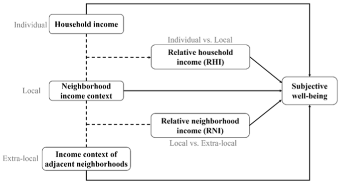
Figure 1 shows the framework of this study. We conceptualize a residential neighborhood as the immediate local context to which its dwellers are exposed, with the neighborhoods embedded within an extra-local context consisting of a collection of adjacent neighborhoods. Because of spatial proximity, the income contexts of both residential and extra-local neighborhoods affect individual well-being through externalities, also referred to as neighborhood effects. The spatial proximity also implies social comparisons of income, generating perceptions of relative (dis)advantages that influence individual well-being. These include comparisons of individuals’ household income with the income context of the residential neighborhood (relative household income (RHI)) and comparisons of income contexts between the residential neighborhood and the extra-local neighborhoods (relative neighborhood income (RNI)). Our research questions are as follows:

(1) Beyond the income context of an individual’s residential neighborhood, what role does the income context of extra-local neighborhoods play in shaping SWB?

(2) In addition to the household’s relative income position within the residential neighborhood (RHI), does the residential neighborhood’s relative income position within its extra-local context (RNI) matter for SWB? How do temporal changes in RHI and RNI influence SWB?

(3) Do the well-being effects of RHI and RNI exhibit symmetric patterns in direction and magnitude? Specifically, are one-unit-higher and one-unit-lower RHI (or RNI) associated with the impact of opposing direction and comparable size on SWB? Does a one-unit positive change in RHI (or RNI) across two time points associate with well-being changes in the opposite direction and with a similar magnitude to a one-unit negative change?

Figure 1.

Research framework.

Method

Study area: Hong Kong

Hong Kong, a special administrative region of China, is the fourth most densely populated city in the world, with 7.4 million residents living within 1111 km², 7% of the total territory.¹ Despite being one of the world’s most affluent cities, Hong Kong has been facing worsening income inequality in recent decades (Piketty and Yang, 2022). These conditions imply that Hong Kong residents live in exceptionally close spatial proximity to one another and are more frequently exposed to extra-local neighborhoods inhabited by people with varying living standards, which heightens residents’ awareness of relative advantage and disadvantage.

Data

We draw on individual-level survey data from the HKPSSD, which is a city-wide representative household panel survey that tracks socioeconomic changes and their impacts on the livelihood of Hong Kong residents (Wu, 2016). The HKPSSD surveyed individuals from a representative household sample obtained through a stratified random sampling method. This sampling method was based on the Frame of Quarters maintained by the Census and Statistics Department, and special attention was paid to the representativeness of the sample in terms of residential location and the population’s socioeconomic status. The data were collected through face-to-face interviews using a computer-assisted personal interviewing system. The first wave of the HKPSSD (W1), completed in 2011, collected information on 7218 respondents aged 15 years or above from 3214 households. The HKPSSD conducted its second wave in 2013 and third wave in 2015, in which a refreshment sample was added. In the fourth wave (W4), conducted from August 2017 to September 2018, 3407 respondents from 2000 households were interviewed.

We use statistics from the quinquennial Hong Kong Population Census aggregated at the large street block group (LSBG) level to measure neighborhood characteristics. LSBG is a statistical unit with a median residential population of approximately 2200 people. Geographical areal data of LSBGs are used to identify adjacent neighborhoods. We also draw on the 100-m resolution gridded population estimates from WorldPop to calculate the population-weighted LSBG centroids. Defining neighborhoods at the LSBG scale captures a shared sense of belonging to the local residential places from general and official perspectives, and this geographical sense of belonging is often tied to perceptions of prestige and social standing. Although this operationalization raises concerns about the modifiable areal unit problem and fuzzy neighborhood boundaries due to human mobility, it is also one motivation for us to include adjacent neighborhoods in the analysis, moving the research focus beyond the arbitrary boundary of a single administratively defined unit to account for the broader spatial context at the localized area that shapes local experiences.

We link the W1 and W4 HKPSSD samples to the 2011 Population Census and 2016 Population By-Census, respectively, based on households’ residential LSBG. After removing cases with missing values for the information we need, we obtain a pooled sample of 8703 observations, consisting of 5652 observations from W1 and 3051 observations from W4. We also construct a balanced panel of 1797 respondents who have participated in both W1 and W4 (3594 person-year observations). The W4 samples in both the pooled sample and balanced panel do not include those who participated in previous waves but moved away from the sampling address,² as the follow-up HKPSSD waves were not eligible to record the movers’ new addresses, making their residential LSBG unknown. Therefore, the contextual effects estimated using the balanced panel are derived solely from temporal changes in the neighborhood characteristics, without capturing the influence of individuals’ self-selection into preferred neighborhoods through relocation.

Measures and analytical approach

Subjective well-being

The dependent variable of this study is individuals’ life satisfaction, which is a valid and reliable measure of individual SWB. The HKPSSD includes the five statements that together constitute the Satisfaction with Life Scale (Diener et al., 1999), and we average the score of the five statements to assess an individual’s cognitive judgment of their satisfaction with life as a whole. The respondents were asked to judge how they felt about each of the statements on a 7-point scale, with 1 indicating “strongly disagree” and 7 indicating “strongly agree.” The five statements are as follows: “I am satisfied with my life,”“So far, I have gotten the important things I want in life,”“In most ways, my life is close to my ideal,”“The conditions of my life are excellent,” and “If I could live my life over, I would change almost nothing.”

Household income

The respondents were asked to report their average monthly household income for the previous year. This includes earnings from all forms of employment, bonuses, commissions, housing or other cash allowances, and various other sources. For those who had difficulties or who were reluctant to give an exact number, a series of income brackets based on household size was provided to select from. For these respondents, we follow Cheung and Lucas (2016) in using the midpoint of their selected bracket as their proximate household income.³

Income contexts of residential neighborhood and adjacent neighborhoods

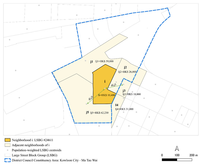
The income context of respondents’ residential neighborhood is measured by the median monthly domestic household income of the LSBG of residence. We follow Graif et al. (2016) and Wang and Arnold (2008) in defining the extra-local context of a given neighborhood as its adjacent neighborhoods and use the weighted average of the adjacent neighborhoods’ median household income to measure the extra-local income context. Adjacent neighborhoods’ income context is calculated as in equation (1). Figure 2 gives an example for illustration.

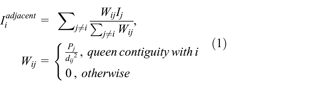
\begin{matrix} I_{i}^{a d j a c e e n t} = \sum_{j \neq i} \frac{W_{i j} I_{j}}{\sum_{j \neq i} W_{i j}}, \\ W_{i j} = {\begin{matrix} \frac{P_{j}}{{d_{i j}}^{2}}, q u e e n c o n t i g u i t y w i t h i \\ 0, o t h e r w i s e \end{matrix} \end{matrix}

(1)

In equation (1), I is the median monthly domestic household income of neighborhood and W_ij is the weight accounting for the geospatial relationship and the relative importance of neighborhood j to i. We use queen contiguity to specify the adjacent neighborhoods that constitute the extra-local context of neighborhood i. In the case shown in Figure 2, the adjacent neighborhoods of neighborhood i are those with shared boundaries (j₁, j₂, j₄, and j₅) and vertices (j₃). The adjacent neighborhoods’ relative importance (i.e. weight) to neighborhood i is assumed to increase with population size, P_j, and to decrease with the squared distance to neighborhood i, $d_{i j}^{2}$ . When calculating d_ij, we account for the within-neighborhood population distribution by using the Euclidean distance between the population-weighted centroids of neighborhoods i and j. In summary, the weight of adjacent neighborhood j for neighborhood i is $\frac{P_{j}}{d_{i j}^{2}}$ .

Figure 2.

Neighborhood and extra-local neighborhoods: An illustration.

Relative household income

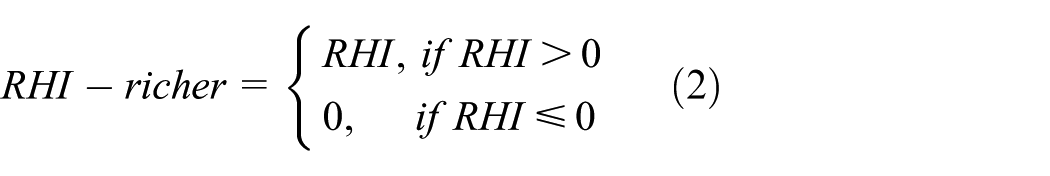
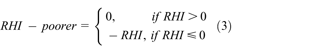
RHI refers to a household’s objective relative income position within the residential neighborhood. It is measured by the distance between the household income and the income context of the residential neighborhood. RHI is therefore a continuous variable with a higher value indicating a higher income position in the local neighborhood context. RHI = 0 is the threshold between the richer and poorer households. We construct the variables RHI-richer and RHI-poorer to test the (a)symmetric pattern of the RHI effects:

R H I - r i c h e r = {\begin{matrix} R H I, & i f R H I > 0 \\ 0, & i f R H I \leq 0 \end{matrix}

(2)

R H I - p o o r e r = {\begin{matrix} 0, & i f R H I > 0 \\ - R H I, & i f R H I \leq 0 \end{matrix}

(3)

Relative neighborhood income

RNI is a geospatial income comparison that accounts for the objective relative income position of a given neighborhood in its extra-local context. A neighborhood’s RNI is measured by the distance between its income context and the income context of its adjacent neighborhoods. RNI is a continuous variable, and the higher its value, the richer a given neighborhood is relative to its surrounding ones. RNI = 0 is the threshold, with a positive value indicating that a neighborhood is richer than adjacent neighborhoods and a negative value indicating a poorer position. Similar to RHI-richer and RHI-poorer, we construct the variables RNI-richer and RNI-poorer to test the (a)symmetric effects of RNI.

Temporal changes in RHI and RNI

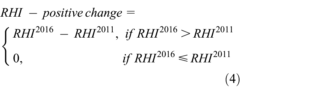
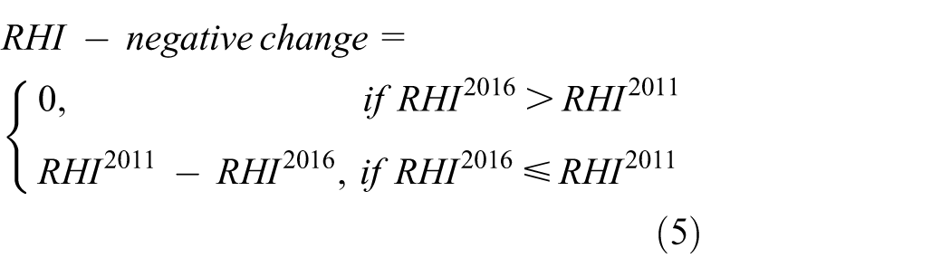
We construct two continuous variables for each of RHI and RNI to indicate the direction and magnitude of their temporal changes between 2011 and 2016. RHI-positive change and RHI-negative change are constructed as in Equations (4) and (5), respectively. The variables RNI-positive change and RNI-negative change have similar definitions.

\begin{matrix} R H I - p o s i t i v e c h a n g e = \\ {\begin{matrix} {R H I}^{2016} - {R H I}^{2011}, & i f {R H I}^{2016} > {R H I}^{2011} \\ 0, & i f {R H I}^{2016} \leq {R H I}^{2011} \end{matrix} \end{matrix}

(4)

\begin{matrix} R H I - n e g a t i v e c h a n g e = \\ {\begin{matrix} 0, & i f {R H I}^{2016} > {R H I}^{2011} \\ {R H I}^{2011} - {R H I}^{2016}, & i f {R H I}^{2016} \leq {R H I}^{2011} \end{matrix} \end{matrix}

(5)

Control variables

We control a set of individual- and neighborhood-level factors that may influence individual SWB. The individual-level factors are sex (male = 1, otherwise 0), age, immigration status (Hong Kong born = 1, otherwise 0), marital status (married = 1, otherwise 0), educational attainment (three categories: lower secondary or below, upper secondary, and tertiary and above), employment status (working = 1, otherwise 0), household size, housing tenure (owner-occupied housing = 1, otherwise 0), and domestic helper employment (yes = 1, otherwise 0). Neighborhood-level factors are neighborhood population density, measured by persons per square meter within an LSBG, and the proportion of rich households in the neighborhood, measured by the proportion of households with a monthly domestic household income of HK$40,000 or above in the LSBG.⁴ We use the proportion of rich households to control for within-neighborhood income distribution, which may confound individuals’ feelings of relative disadvantage.

Analytical approach

We first report the summary statistics of the pooled sample and balanced panel for W1 and W4 to present an overview of our analytical samples. We then conduct ordinary least squares (OLS) regressions to estimate the SWB effects of the geospatial relative income. Analyses based on the pooled sample examine the relationship between geospatial relative income and SWB, with individual- and neighborhood-level characteristics controlled and the standard errors clustered by individual. Analyses based on the balanced panel use first-difference regressions to investigate the SWB effects of the temporal changes in geospatial relative income from 2011 to 2016, addressing unobserved heterogeneities.

Results

Descriptive statistics

Figure 3(a) presents the RNI range of all neighborhoods in Hong Kong in 2011. Given that RNI is a localized concept, any relatively poorer neighborhood (shaded in blue) is adjacent to at least one relatively richer neighborhood (shaded in red with a dotted pattern), and vice versa. Figure 3(b) shows the neighborhoods covered by the pooled sample and their RNI range in 2011. Figure 3(c) displays the neighborhoods covered by the balanced panel and the direction of their change in RNI from 2011 to 2016. Neighborhoods with a negative temporal change in RNI are shown in yellow, and those with a positive temporal change are shown in purple with a crosshatch pattern. Neighborhoods with no analytical sample are unshaded, most of which are in hilly to mountainous areas and consisting mainly of woodland, grassland, farmland, and/or country parks or nature reserves as indicated by the light-green raster layer. Both the pooled sample and the balanced panel are distributed across most of the populated neighborhoods in Hong Kong, although the balanced panel is smaller and covers fewer neighborhoods.

Figure 3.

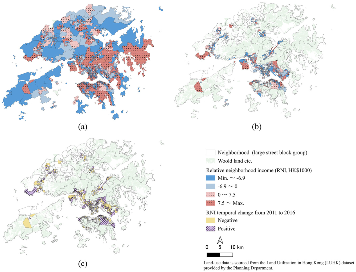
Relative neighborhood income of neighborhoods in Hong Kong: (a) RNI range of all neighborhoods in Hong Kong in 2011, (b) neighborhoods covered by the pooled sample and their RNI range in 2011, and (c) neighborhoods covered by the balanced panel and the direction of their change in RNI from 2011 to 2016.

Comparing the W1 observations of the balanced panel with the pooled sample (Table 1), we find that the balanced panel has fewer male respondents (0.45 vs 0.48), an older average age (47.86 vs 45.20), more married respondents (0.67 vs 0.59), fewer working respondents (0.50 vs 0.52) from smaller households (3.35 vs 3.48), a higher proportion of respondents with lower secondary education or below (51.4% vs 49.4%), and a lower proportion of respondents with tertiary education and above (10.7% vs 12.4%). For the W4 observations, the balanced panel is older (54.38 vs 51.86), less likely to be born in Hong Kong (0.56 vs 0.58), and more likely to be married (0.69 vs 0.63) and working (0.54 vs 0.51). Other individual-level characteristics, as well as residential neighborhoods’ population density and the proportion of richer households, are almost identical between the pooled and balanced samples.

Table 1.

Summary statistics.

	Pooled sample (N = 8703)		Balanced panel (N = 3594)
	W1 (N = 5652)	W4 (N = 3051)	W1 (N = 1797)	W4 (N = 1797)
Subjective well-being (SWB)	4.58 (1.13)	4.68 (1.12)	4.66 (1.14)	4.70 (1.11)
Household income (HK$1000)	26.66 (27.25)	29.50 (26.45)	25.76 (31.37)	30.38 (25.78)
Relative household income (RHI, HK$1000)	1.95 (25.21)	6.01 (24.73)	2.18 (28.95)	6.87 (23.89)
Neighborhood income level (HK$1000)	24.72 (13.79)	23.48 (10.70)	23.58 (12.19)	23.51 (10.30)
Relative neighborhood income (RNI, HK$1000)	−2.74 (12.77)	−2.56 (10.45)	−3.22 (12.77)	−2.85 (10.33)
Adjacent neighborhoods’ income level (HK$1000)	27.46 (11.94)	26.04 (9.18)	26.80 (11.01)	26.35 (9.13)
Male	0.48 (0.50)	0.45 (0.50)	0.45 (0.50)	0.45 (0.50)
Age	45.20 (18.21)	51.86 (18.69)	47.86 (16.75)	54.38 (16.70)
Hong Kong born	0.57 (0.49)	0.58 (0.49)	0.56 (0.50)	0.56 (0.50)
Married	0.59 (0.49)	0.63 (0.48)	0.67 (0.47)	0.69 (0.46)
Working	0.52 (0.50)	0.51 (0.50)	0.50 (0.50)	0.54 (0.50)
Education—lower secondary or below	49.4%	47.1%	51.4%	47.2%
Education—upper secondary	38.2%	38.7%	37.9%)	37.8%
Education—tertiary and above	12.4%	14.2%	10.7%)	15.0%
Household size	3.48 (1.33)	3.42 (1.41)	3.35 (1.27)	3.40 (1.33)
Owner-occupied housing	0.52 (0.50)	0.51 (0.50)	0.51 (0.50)	0.52 (0.50)
Domestic helper employment	0.12 (0.32)	0.10 (0.30)	0.13 (0.33)	0.11 (0.31)
Neighborhood population density	0.12 (0.08)	0.12 (0.08)	0.12 (0.08)	0.12 (0.08)
Prop. of rich households in the neighborhood	0.17 (0.17)	0.25 (0.16)	0.16 (0.17)	0.25 (0.16)

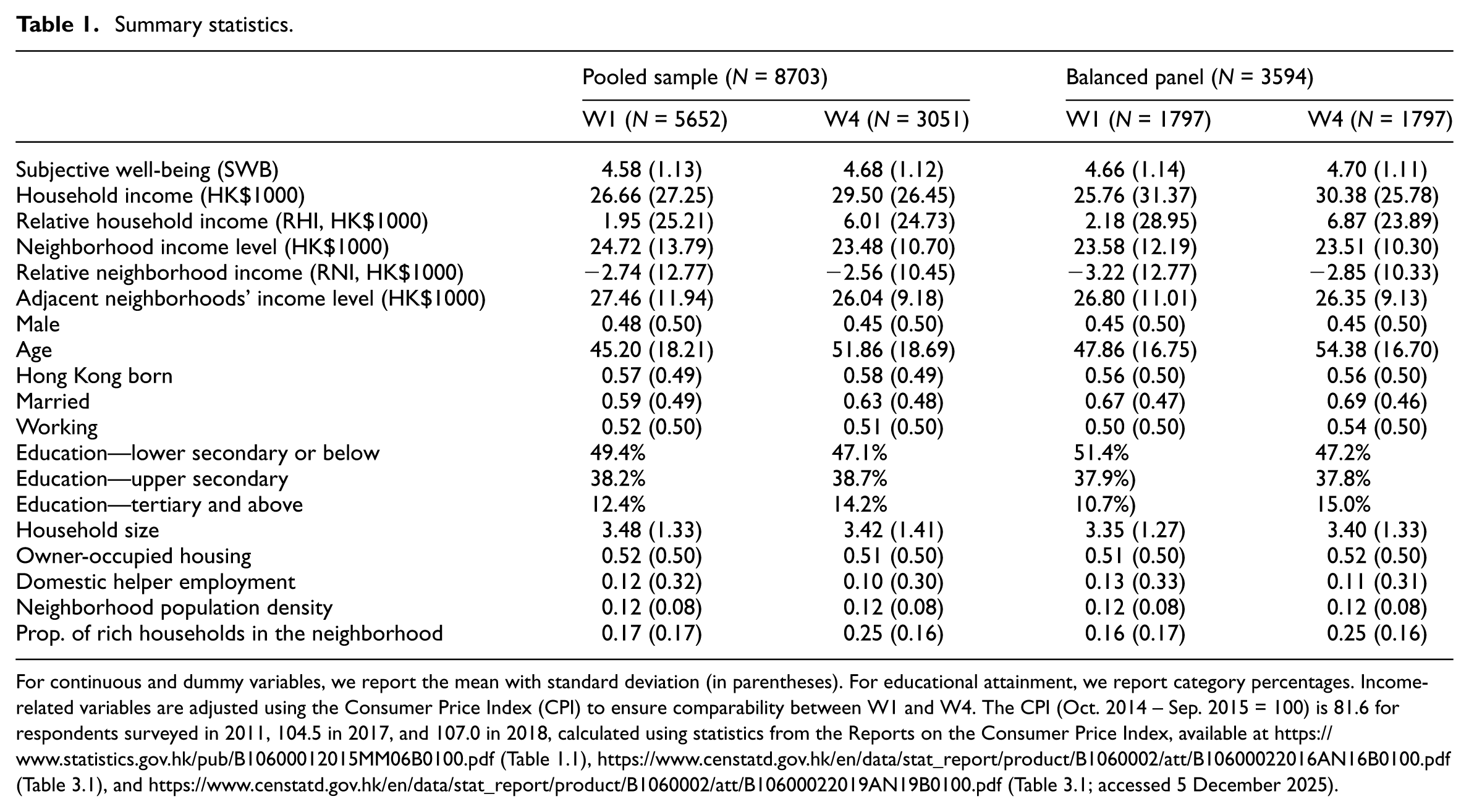
For continuous and dummy variables, we report the mean with standard deviation (in parentheses). For educational attainment, we report category percentages. Income-related variables are adjusted using the Consumer Price Index (CPI) to ensure comparability between W1 and W4. The CPI (Oct. 2014 – Sep. 2015 = 100) is 81.6 for respondents surveyed in 2011, 104.5 in 2017, and 107.0 in 2018, calculated using statistics from the Reports on the Consumer Price Index, available at https://www.statistics.gov.hk/pub/B10600012015MM06B0100.pdf (Table 1.1), https://www.censtatd.gov.hk/en/data/stat_report/product/B1060002/att/B10600022016AN16B0100.pdf (Table 3.1), and https://www.censtatd.gov.hk/en/data/stat_report/product/B1060002/att/B10600022019AN19B0100.pdf (Table 3.1; accessed 5 December 2025).

The mean SWB values of the pooled sample and the balanced panel in W1 are 4.58 (SD = 1.13) and 4.66 (SD = 1.14), respectively. From W1 to W4, we observe a 0.1 increase in the mean SWB for the pooled sample and 0.04 for the balanced panel. The average monthly household income is HK$29,500 for the pooled sample in W4, which is HK$2840 higher than that in W1. For the balanced panel, W4 has an average monthly household income of HK$30,380, which is HK$4620 higher than W1. Regarding the residential neighborhood income level, the mean temporal changes from W1 to W4 are HKfdeminus;1240 (from HK$24,720 to HK$23,480) for the pooled sample and HK$70 (HK$23,580 to HK$23,510) for the balanced panel. The temporal changes in adjacent neighborhoods’ income context are HKfdeminus;1420 (HK$27,460 to HK$26,040) and HK$450 (HK$26,800 to HK$26,350) for the pooled and balanced panels, respectively.

As indicated by the temporal changes and the standard deviations, there is more variation in household income than in the income levels of residential neighborhood and adjacent neighborhoods. As a result, we observe more variation in RHI than in RNI: for RHI, it is around HK$2000 in W1 and increases to above HK$6000 in W4 for both the pooled sample and the balanced panel; for RNI, it is HKfdeminus;2740 in W1 and HKfdeminus;2560 in W4 for the pooled sample, and HKfdeminus;3220 in W1 and HKfdeminus;2850 in W4 for the balanced panel. The standard deviations of RHI are double those of RNI, suggesting greater inter-personal heterogeneities than inter-neighborhood heterogeneities in terms of both absolute and relative income.

Geospatial relative income and individual SWB

Table 2 presents the results of four model specifications using the pooled sample with standard errors clustered by individuals. Model 1 shows significant overall SWB effects of household income (0.004, p < 0.001), neighborhood income level (0.009, p < 0.01), and adjacent neighborhoods’ income level (−0.002, p < 0.05), controlling for individual- and neighborhood-level characteristics. Model 2 includes RHI and RNI to replace the income-related variables in absolute terms. The coefficients of RHI and RNI are identical in terms of direction and magnitude, implying that they are equally important predictors of individual SWB. The RHI coefficient suggests that compared with people with a household income equal to the neighborhood income level (RHI = 0), people with a household income that is HK$1000 higher (RHI = 1) tend to have a 0.004 higher SWB score (p < 0.001). The RNI coefficient suggests that compared with people living in a neighborhood with an income level equal to the adjacent neighborhoods’ income level (RNI = 0), people living in a neighborhood with an income level that is HK$1000 higher (RNI = 1) tend to have a 0.004 higher SWB score (p < 0.01).

Table 2.

Multivariable linear regression for subjective well-being using the pooled sample.

	Model 1	Model 2	Model 3	Model 4
Household income	0.004*** (0.001)			0.004*** (0.001)
RHI		0.004*** (0.000)
RHI-richer			0.003*** (0.001)
RHI-poorer			−0.008*** (0.002)
Neighborhood income level	0.009** (0.003)			0.008* (0.003)
RNI		0.004** (0.001)
RNI-richer			0.003 (0.002)	−0.001 (0.003)
RNI-poorer			−0.004* (0.002)	−0.004** (0.002)
Adjacent neighborhoods’ income level	−0.002* (0.001)
Control variables
Male	−0.138*** (0.025)	−0.139*** (0.025)	−0.139*** (0.025)	−0.138*** (0.025)
Age	−0.001 (0.001)	−0.001 (0.001)	−0.001 (0.001)	−0.001 (0.001)
Hong Kong born	0.110*** (0.028)	0.111*** (0.028)	0.107*** (0.028)	0.109*** (0.028)
Married	0.238*** (0.030)	0.237*** (0.030)	0.229*** (0.030)	0.239*** (0.030)
Working	−0.168*** (0.026)	−0.166*** (0.026)	−0.174*** (0.027)	−0.168*** (0.026)
Education attainment (ref. = upper secondary)
Lower secondary or below	−0.026 (0.030)	−0.026 (0.030)	−0.025 (0.030)	−0.025 (0.030)
Tertiary and above	0.029 (0.040)	0.036 (0.040)	0.035 (0.040)	0.028 (0.040)
Household size	−0.012 (0.010)	−0.009 (0.010)	−0.013 (0.010)	−0.012 (0.010)
Owner-occupied housing	0.210*** (0.029)	0.200*** (0.029)	0.196*** (0.029)	0.204*** (0.029)
Domestic helper employment	0.198*** (0.039)	0.203*** (0.039)	0.201*** (0.039)	0.198*** (0.039)
Neighborhood population density	−0.457** (0.158)	−0.470** (0.158)	−0.470** (0.158)	−0.471** (0.157)
Prop. of rich households in the neighborhood	−0.062 (0.234)	0.660*** (0.097)	0.781*** (0.114)	−0.062 (0.236)
Wave 4	0.083** (0.032)	0.017 (0.025)	0.003 (0.026)	0.080* (0.032)
R ²	0.082	0.080	0.081	0.082
Number of observations	8703	8703	8703	8703

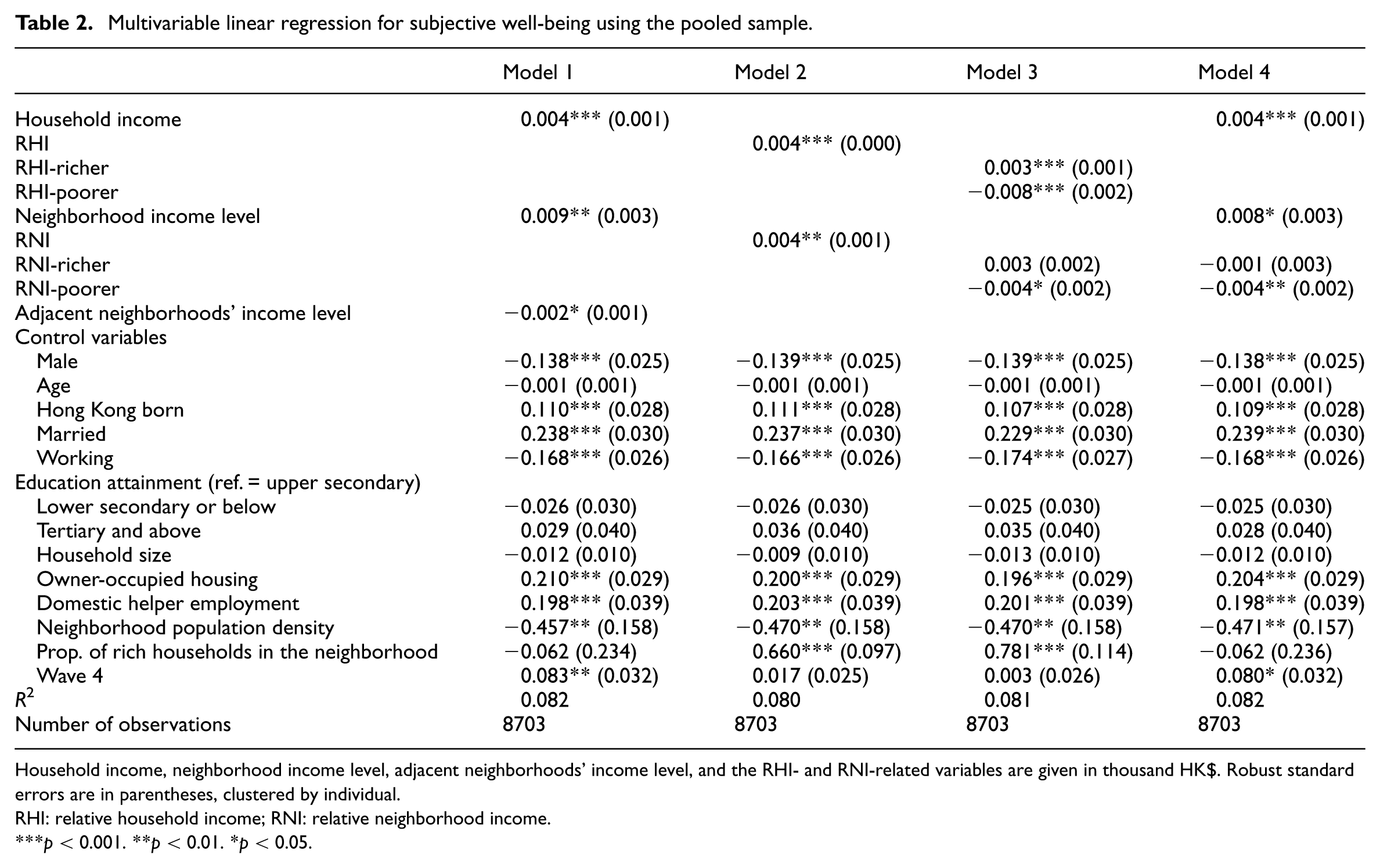
Household income, neighborhood income level, adjacent neighborhoods’ income level, and the RHI- and RNI-related variables are given in thousand HK$. Robust standard errors are in parentheses, clustered by individual.

RHI: relative household income; RNI: relative neighborhood income.

***

p < 0.001. **p < 0.01. *p < 0.05.

Next, we replace RHI and RNI with the sets of richer/poorer variables to examine the (a)symmetric patterns of the effects (Model 3). The statistically significant coefficients of RHI-richer (0.003, p < 0.001) and RHI-poorer (−0.008, p < 0.001) suggest that the RHI effect has a weak symmetric pattern, with upward comparison more pronounced in terms of magnitude. Specifically, compared with people with a household income less than or equal to the neighborhood’s income level (RHI-richer = 0, i.e. RHI ≤ 0), people with a household income that is HK$1000 higher (RHI-richer = 1) tend to have a 0.003 higher SWB score; compared with people with a household income higher than the neighborhood’s income level (RHI-poorer = 0, i.e. RHI > 0), people with a household income that is HK$1000 lower (RHI-poorer = 1) tend to have a 0.008 lower SWB score.

For RNI, we observe a positive but nonsignificant coefficient of RNI-richer (0.003) and a statistically significant negative coefficient of RNI-poorer (−0.004, p < 0.05) in Model 3. Because the focus of this study is on RNI, we further estimate the lower bounds of the pure RNI effects that separate the positive externalities of neighborhood income level. In Model 4, we keep the RNI variables but replace the RHI variables with household income and neighborhood income level. The coefficient of neighborhood income level in this specification absorbs the positive externalities of the neighborhood. As a result, the RNI coefficient, combining the pure RNI effects and the positive externalities of adjacent neighborhoods, is the lower bound of the pure RNI effects on SWB. For RNI-richer, the lower bound is a non-significant estimate of −0.001, while for RNI-poorer, it is a significant estimate of −0.004 (p < 0.01). This suggests that the RNI effect shows an asymmetric pattern in terms of statistical significance, with only upward comparisons related to significantly lower SWB. Specifically, compared with people living in a neighborhood with an income context that is richer than the adjacent neighborhoods (RNI-poorer = 0, i.e. RNI > 0), people living in a neighborhood with an income context that is HK$1000 lower (RNI-poorer = 1) tend to have a 0.004 lower SWB score.

The coefficients of the income-related variables in Table 2 are small in magnitude, a finding further confirmed by their corresponding elasticity estimates calculated at the mean. For example, in Table 2, for Model 3, the elasticity estimates are 0.006 for RHI-richer, −0.010 for RHI-poorer, 0.002 for RNI-richer, and −0.005 for RNI-poorer. The pooled OLS estimators are derived from both within- and between-individual variations. Therefore, the small magnitudes of the effects are probably due to the confounded influence of unobserved, time-invariant individual characteristics—such as personality traits and genetic factors—that are correlated with both the income-related factors and SWB.

The results in Table 2 also show that SWB is higher for married respondents, Hong Kong-born respondents, and respondents from a household that owns the residential house and employs a domestic helper, but it is lower among male respondents and working respondents. The findings for sex, marital status, and employment status are consistent with those of previous studies in Hong Kong (Miao and Wu, 2022; Wang et al., 2019). The positive effect of homeownership echoes a study of the Hong Kong Ownership Scheme (Miao and Wu, 2022). The finding of higher SWB among Hong Kong natives aligns with the study of Zeng and Zhang (2022), suggesting that migrants in Hong Kong are disadvantaged in terms of both objective (Zhang and Wu, 2011; Zhang and Ye, 2018) and subjective outcomes. The SWB of Hong Kong residents does not significantly differ by educational attainment, which is consistent with the findings of Zeng and Zhang (2022).

Neighborhood population density is negatively associated with individual SWB. As shown in Table 2, for Model 2 and Model 3, which do not include any of the income variables in absolute terms, the proportion of rich households in a neighborhood has a significant positive coefficient, reflecting the positive effect of the neighborhood’s income level. In Models 1 and 4, the proportion of rich households controls the extreme income structure within the neighborhood and yields negative and nonsignificant coefficients.

Temporal changes in geospatial relative income and individual SWB

Table 3 reports the first-difference estimators of four model specifications using the balanced panel data.⁵ Model 1 shows that for increases of HK$1000 in household income and the neighborhood income level from W1 to W4, individuals’ SWB score increases significantly, by 0.003 (p < 0.05) and 0.018 (p < 0.05), respectively, and a change in extra-local neighborhoods’ income level exerts an overall SWB effect that is negative and statistically nonsignificant (−0.006). In Model 2, the absolute income variables are replaced with RHI and RNI, and positive and statistically significant coefficients are found for both RHI (0.003, p < 0.01) and RNI (0.012, p < 0.05). The coefficient of RHI in Model 2 suggests that for the same individual, a HK$1000 change in RHI over time is associated with a change in SWB of 0.003 in the same direction. However, we find that the symmetric pattern is weak: when RHI is replaced with the RHI-positive/negative change variables (Model 3), we obtain coefficients of RHI-positive change and RHI-negative change that point in opposing directions but lack statistical significance.

Table 3.

First-difference estimators of the impact of temporal change in geospatial relative income on subjective well-being using the balanced panel data.

	Model 1	Model 2	Model 3	Model 4
Household income	0.003* (0.001)			0.003** (0.001)
RHI		0.003** (0.001)
RHI-positive change			0.003 (0.002)
RHI-negative change			−0.002 (0.001)
Neighborhood income level	0.018* (0.008)			0.023* (0.011)
RNI		0.012* (0.006)
RNI-positive change			0.024** (0.009)	0.021* (0.009)
RNI-negative change			0.002 (0.009)	0.021 (0.012)
Adjacent neighborhoods’ income level	−0.006 (0.007)
Control variables	Yes	Yes	Yes	Yes
R ²	0.013	0.012	0.014	0.017
Number of waves	2	2	2	2
Number of individuals	1797	1797	1797	1797
Number of observations	3594	3594	3594	3594

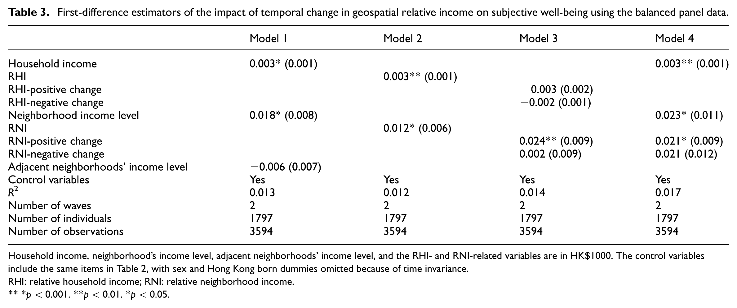
Household income, neighborhood’s income level, adjacent neighborhoods’ income level, and the RHI- and RNI-related variables are in HK$1000. The control variables include the same items in Table 2, with sex and Hong Kong born dummies omitted because of time invariance.

RHI: relative household income; RNI: relative neighborhood income.

***

p < 0.001. **p < 0.01. *p < 0.05.

For RNI, we find an asymmetric pattern that individual SWB is more affected by positive RNI changes and less sensitive to negative RNI changes. Model 3 shows that an increase in RNI from W1 to W4 by HK$1000 relates to a 0.024 (p < 0.01) increase in SWB, while a decrease does not bring a significant SWB change (0.002). We further test the RNI effects by estimating the lower bounds for the pure effects of RNI temporal changes in Model 4. When controlling for the temporal changes in household income and neighborhood income level from W1 to W4, the coefficients of RNI-positive/negative change are the lower-bound estimations that incorporate the externalities of adjacent neighborhoods. We obtain a statistically significant lower-bound estimation of 0.021 (p < 0.05) for the pure effect of a positive RNI change by HK$1000 and a nonsignificant estimate for a negative RNI change. This confirms the finding that from a temporal perspective, RNI affects individual SWB mainly through upward changes. The nonsignificant effects of RNI-negative change and its positive coefficients in Models 3 and 4 imply that the positive externalities of adjacent neighborhoods may play a role in offsetting the negative effect of a decrease in RNI.

The first-difference estimators of the income-related variables based on the balanced panel (Table 3) are larger than the pooled OLS estimators in Table 2. This is confirmed by the elasticities estimated at the mean. For example, Table 3 Model 3 yields elasticity estimates of 0.800 for RHI-positive change, −0.350 for RHI-negative change, 1.447 for RNI-positive change, and 0.099 for RNI-negative change. Focusing on within-individual variation over time, the first-difference estimators suggest that for a given individual, SWB changes with the temporal changes in RHI and RNI and is particularly sensitive to RNI-positive change, where a 1% increase over time is associated with a 1.447% rise in SWB.

Conclusion and discussion

SWB is a complex and comprehensive indicator of people’s subjective evaluation of their lives based on their material standard of living (Diener et al., 2013; Jebb et al., 2018; Kahneman and Deaton, 2010; Killingsworth, 2021; Stevenson and Wolfers, 2013), working status (Kamerāde and Richardson, 2018; Zhang et al., 2023), life course experiences (Buecker et al., 2023; Gurven et al., 2024), and other factors (Helliwell et al., 2012, 2017). Income level largely determines people’s living conditions and social standing, contributing to SWB both directly and indirectly through social comparison with others. This study focuses on the SWB effects of geographical relative income at the neighborhood level and extends the literature by accounting for the spatiotemporal influences of the income context of extra-local neighborhoods.

Using two waves of geocoded survey data in Hong Kong linked with official neighborhood-level statistics, we find that household income and the income contexts of residential neighborhood and the adjacent neighborhoods matter for individual SWB, and both the RHI (the household’s relative income position within the residential neighborhood) and the RNI (the residential neighborhood’s relative income position compared with its adjacent neighborhoods) have positive SWB effects. Empirically, we observe positive overall effects for household income and neighborhood income level and a negative overall effect for the income level of the adjacent neighborhoods. These findings suggest that a higher-income context of adjacent neighborhoods induces a negative SWB effect by lowering RNI, which outweighs the positive externalities it generates. This finding provides consistent empirical evidence of a positive overall effect of the local neighborhood and a negative overall effect of other more distant neighborhoods (Crowder and South, 2011; Kingdon and Knight, 2007; South and Crowder, 2010). We also find that the magnitudes of these SWB effects are consistently larger for the geospatial relative income measures than for the absolute income measures, and the most substantial SWB effects are observed for positive temporal changes in RNI.

We observe weak symmetric patterns for the SWB effects of RHI. The upward comparison effect (i.e. the household being poorer within the residential neighborhood is associated with a lower SWB) is more pronounced than the downward comparison effect (i.e. a household being richer within the residential neighborhood is associated with a higher SWB). This provides empirical evidence supporting Dusenberry’s idea that comparisons are mostly upward (Distante, 2013; Ferrer-i-Carbonell, 2005). However, from a temporal perspective, we find that neither a positive nor a negative temporal change in RHI is significantly related to changes in SWB.

For RNI, we observe asymmetric patterns in the SWB effects that upward comparisons and positive temporal changes are more pronounced. Specifically, upward comparisons with richer neighborhoods adjacent to the residential neighborhood (i.e. the residential neighborhood is relatively poorer than the adjacent neighborhoods) are associated with significantly lower SWB, while the relationship between downward comparisons (i.e. the residential neighborhood is relatively richer than the adjacent neighborhoods) and SWB is positive but not statistically significant. From a temporal perspective, an improvement in the residential neighborhood’s relative income position is linked with a significant increase in SWB, whereas a decline in the relative position does not correspond to a significant difference in SWB.

The local and extra-local contexts of residency, around which everyday life is structured and organized, form a sense of belonging that can shape perceptions of subjective socioeconomic status (Roy et al., 2016). Therefore, a residential neighborhood with a higher income level than its adjacent neighborhoods can reinforce residents’ perceptions of relative advantage, exerting positive effects on their SWB. Although a negative temporal change in RNI is not linked to significant decreases in SWB, possibly because of the offsetting effects of the positive externalities generated by richer adjacent neighborhoods, our findings also imply that people living in neighborhoods with relatively poorer income positions will continue to have relatively low SWB if their residential neighborhoods experience no improvement in relative income position over time. In light of these, we recommend policymakers monitor the evolution of neighborhood income contexts and pay attention to the social comparisons generated from spatially structured disadvantages at microgeographical levels. It is important to invest in public services and infrastructure and to implement urban renewal plans for disadvantaged neighborhoods, with special attention paid to those experiencing further deterioration in the extra-local context during the process of urban development. By improving the physical environment of relatively disadvantaged neighborhoods, these efforts can enhance residents’ well-being and attract residents with higher socioeconomic status, fostering social mixing and reducing inter-neighborhood income inequality.

We acknowledge several limitations of this study that should be addressed in future research. One limitation is sample attrition. Additional analysis shows that although there is no significant difference in absolute household income or the two dimensions of geospatial relative income, the retained respondents have higher SWB than the respondents who dropped out, and they differ in some sociodemographic factors. This suggests that our estimation may be subject to bias. We hope that future social panel surveys will use enhanced tracking methods to mitigate attrition and improve the representativeness of longitudinal data. Another data limitation stems from our inability to obtain the W4 residential addresses of respondents who moved. Our analysis, focused on non-movers, does not capture the well-being changes associated with strategic residential self-selection. We recommend that future work collect more comprehensive data to study this selection process directly. In addition, the contextual influences of the dynamic activity spaces (e.g. places that people visit daily for work, school, shopping, and leisure) merit further investigation, which will entail the collection of data on individuals’ daily activities and mobility.

Despite these limitations, this study has theoretical implications that highlight the importance of the wider sociospatial contexts beyond residential neighborhoods and their interactions with residential neighborhoods in neighborhood effect studies. It also provides empirical evidence to discuss the UGCoP and SPACEs that can inform both conceptual development and planning practices concerning the interplay between people, space, and time.

Footnotes

Acknowledgements

We are grateful to the discussants at the KUIGE Forum (2024, Yunnan University), the editors, and the anonymous referees for their helpful comments and suggestions. The authors would like to thank the Center for Applied Social and Economic Research at the Hong Kong University of Science and Technology for granting access to data from the Hong Kong Panel Study of Social Dynamics.

ORCID iDs

Chi Zhang

Zhuoni Zhang

Funding

The authors disclosed receipt of the following financial support for the research, authorship, and/or publication of this article: This study is supported by the AI Research and Learning Base of Urban Culture (project 2023WZJD008), the Guangzhou Municipal Science and Technology Project (Guangzhou Basic and Applied Basic Research Scheme, nos. 2024A04J6375 and 2025A03J3490, principal investigator: Zhuoni Zhang), the High-End Foreign Experts Introduction Program of the State Administration of Foreign Experts Affairs, Ministry of Science and Technology, China (no. G2023030045L, principal investigator: Zhuoni Zhang), and a Key Project, “Research on Population Structure and Mobility Pattern in the Great Bay Area,” from the China Ministry of Education, Research Base in Humanities and Social Science (22JJD 840013).

Declaration of conflicting interests

The authors declared no potential conflicts of interest with respect to the research, authorship, and/or publication of this article.

Notes

References

Asadullah

Xiao

Yeoh

(2018) Subjective well-being in China, 2005–2010: The role of relative income, gender, and location. China Economic Review 48: 83–101.

Brown

Gray

Roberts

(2015) The relative income hypothesis: A comparison of methods. Economics Letters 130: 47–50.

Buecker

Luhmann

Haehner

, et al. (2023) The development of subjective well-being across the life span: A meta-analytic review of longitudinal studies. Psychological Bulletin 149(7–8): 418–446.

Cheung

Lucas

(2016) Income inequality is associated with stronger social comparison effects: The effect of relative income on life satisfaction. Journal of Personality and Social Psychology 110(2): 332–341.

Clark

Senik

(2010) Who compares to whom? The anatomy of income comparisons in Europe. Economic Journal 120(544): 573–594.

Clark

Frijters

Shields

(2008) Relative income, happiness, and utility: An explanation for the Easterlin paradox and other puzzles. Journal of Economic Literature 46(1): 95–144.

Clark

Kristensen

Westergård-Nielsen

(2009) Economic satisfaction and income rank in small neighbourhoods. Journal of the European Economic Association 7(2–3): 519–527.

Crowder

South

(2011) Spatial and temporal dimensions of neighborhood effects on high school graduation. Social Science Research 40(1): 87–106.

Deaton

Stone

(2013) Two happiness puzzles. American Economic Review 103(3): 591–597.

10.

Diener

Suh

Lucas

, et al. (1999) Subjective well-being: Three decades of progress. Psychological Bulletin 125(2): 276–302.

11.

Diener

Tay

Oishi

(2013) Rising income and the subjective well-being of nations. Journal of Personality and Social Psychology 104(2): 267–276.

12.

Dietz

(2002) The estimation of neighborhood effects in the social sciences: An interdisciplinary approach. Social Science Research 31(4): 539–575.

13.

Distante

(2013) Subjective well-being, income and relative concerns in the UK. Social Indicators Research 113(1): 81–105.

14.

Easterlin

(1974) Does economic growth improve the human lot? Some empirical evidence. In: David

Reder

(eds) Nations and Households in Economic Growth. Elsevier, pp.89–125.

15.

Easterlin

(1995) Will raising the incomes of all increase the happiness of all? Journal of Economic Behavior & Organization 27(1): 35–47.

16.

Easterlin

(2003) Explaining happiness. Proceedings of the National Academy of Sciences of the United States of America 100(19): 11176–11183.

17.

Easterlin

(2013) Happiness, growth, and public policy. Economic Inquiry 51(1): 1–15.

18.

Easterlin

Sawangfa

(2010) Happiness and economic growth: Does the cross section predict time trends? Evidence from developing countries. In: Diener

Kahneman

Helliwell

(eds) International Differences in Well-Being. Oxford University Press, pp.166–216.

19.

Ferrer-i-Carbonell

(2005) Income and well-being: An empirical analysis of the comparison income effect. Journal of Public Economics 89(5–6): 997–1019.

20.

Festinger

(1954) A theory of social comparison processes. Human Relations 7(2): 117–140.

21.

Graif

Arcaya

Diez Roux

(2016) Moving to opportunity and mental health: Exploring the spatial context of neighborhood effects. Social Science and Medicine 162: 50–58.

22.

Gurven

Buoro

Rodriguez

, et al. (2024) Subjective well-being across the life course among non-industrialized populations. Science Advances 10(43): eado0952.

23.

Helliwell

Layard

Sachs

(2012) World Happiness Report. UN Sustainable Development Solutions Network.

24.

Helliwell

Layard

Sachs

(2017) World Happiness Report 2017. Sustainable Development Solutions Network.

25.

Howell

(2008) The relation of economic status to subjective well-being in developing countries: A meta-analysis. Psychological Bulletin 134(4): 536–560.

26.

Huang

Deng

(2016) Relative income, relative assets, and happiness in urban China. Social Indicators Research 126(3): 971–985.

27.

Inagami

Cohen

Finch

(2007) Non-residential neighborhood exposures suppress neighborhood effects on self-rated health. Social Science and Medicine 65(8): 1779–1791.

28.

Jebb

Tay

Diener

, et al. (2018) Happiness, income satiation and turning points around the world. Nature Human Behaviour 2(1): 33–38.

29.

Kahneman

Deaton

(2010) High income improves evaluation of life but not emotional well-being. Proceedings of the National Academy of Sciences of the United States of America 107(38): 16489–16493.

30.

Kamerāde

Richardson

(2018) Gender segregation, underemployment and subjective well-being in the UK labour market. Human Relations 71(2): 285–309.

31.

Killingsworth

(2021) Experienced well-being rises with income, even above $75,000 per year. Proceedings of the National Academy of Sciences of the United States of America 118(4): 1–6.

32.

Kingdon

Knight

(2007) Community, comparisons and subjective well-being in a divided society. Journal of Economic Behavior & Organization 64(1): 69–90.

33.

Kwan

(2012) The uncertain geographic context problem. Annals of the Association of American Geographers 102(5): 958–968.

34.

Kwan

(2018) The limits of the neighborhood effect: Contextual uncertainties in geographic, environmental health, and social science research. Annals of the American Association of Geographers 108(6): 1482–1490.

35.

Latif

(2016) Happiness and comparison income: Evidence from Canada. Social Indicators Research 128(1): 161–177.

36.

Luttmer

EFP

(2005) Neighbors as negatives: Relative earnings and well-being. Quarterly Journal of Economics 120(3): 963–1002.

37.

McBride

(2001) Relative-income effects on subjective well-being in the cross-section. Journal of Economic Behavior & Organization 45(3): 251–278.

38.

Matthews

Yang

(2013) Spatial Polygamy and Contextual Exposures (SPACEs): Promoting activity space approaches in research on place and health. American Behavioral Scientist 57(8): 1057–1081.

39.

Metz

Burdina

(2018) Neighbourhood income inequality and property crime. Urban Studies 55(1): 133–150.

40.

Miao

(2024) Socio-spatial differentiation and residential inequalities in Chinese cities. Sociology Compass 18(2): e13174.

41.

Miao

(2022) Social consequences of homeownership: Evidence from the home ownership scheme in Hong Kong. Social Forces 101(3): 1460–1484.

42.

Petrović

Manley

Van Ham

(2020) Freedom from the tyranny of neighbourhood: Rethinking sociospatial context effects. Progress in Human Geography 44(6): 1103–1123.

43.

Piketty

Yang

(2022) Income and wealth inequality in Hong Kong, 1981–2020: The rise of Pluto-Communism? World Bank Economic Review 36(4): 803–834.

44.

Roy

Godfrey

Rarick

JRD

(2016) Do we know where we stand? Neighborhood relative income, subjective social status, and health. American Journal of Community Psychology 57(3–4): 448–458.

45.

Schwanen

Wang

(2014) Well-being, context, and everyday activities in space and time. Annals of the Association of American Geographers 104(4): 833–851.

46.

Sharkey

Faber

(2014) Where, when, why, and for whom do residential contexts matter? Moving away from the dichotomous understanding of neighborhood effects. Annual Review of Sociology 40: 559–579.

47.

South

Crowder

(2010) Neighborhood poverty and nonmarital fertility: Spatial and temporal dimensions. Journal of Marriage and Family 72: 89–104.

48.

Stevenson

Wolfers

(2008) Economic growth and subjective well-being: Reassessing the Easterlin paradox. Brookings Papers on Economic Activity 39: 1–87.

49.

Stevenson

Wolfers

(2013) Subjective well-being and income: Is there any evidence of satiation? American Economic Review 103(3): 598–604.

50.

Tsurumi

Imauji

Managi

(2019) Relative income, community attachment and subjective well–being: Evidence from Japan. Kyklos 72(1): 152–182.

51.

Veenhoven

Hagerty

(2006) Rising happiness in nations 1946–2004: A reply to Easterlin. Social Indicators Research 79(3): 421–436.

52.

Wang

Schwanen

Mao

(2019) Does exposure to richer and poorer neighborhoods influence wellbeing? Cities 95: 102408.

53.

Wang

Arnold

(2008) Localized income inequality, concentrated disadvantage and homicide. Applied Geography 28(4): 259–270.

54.

(2016) Hong Kong Panel Study of Social Dynamics (HKPSSD): Research designs and data overview. Chinese Sociological Review 48(2): 162–184.

55.

Zeng

Zhang

(2022) Neighborhood socioeconomic status, relative household income, and life satisfaction of Chinese mainland migrants in Hong Kong. Chinese Journal of Sociology 8(2): 165–186.

56.

Zhang

Piao

Managi

(2023) Work Hour Mismatch on Life Evaluation: Full Heterogeneity and Individual- and Country-Level Characteristics of the Most and Least Affected Workers. Springer Netherlands.

57.

Zhang

Miao

(2025) From disorder to distress: Investigating neighborhood change and mental health with Streetview and longitudinal survey data. Social Science and Medicine 384: 118589.

58.

Zhang

(2026) Public housing and neighborhood composition in Hong Kong, 1981–2016. Social Science Research 133: 103276.

59.

Zhang

(2011) Social change, cohort quality and economic adaptation of Chinese immigrants in Hong Kong, 1991–2006. Asian and Pacific Migration Journal 20(1): 1–29.

60.

Zhang

(2018) Mode of migration, age at arrival, and occupational attainment of immigrants from Mainland China to Hong Kong. Chinese Sociological Review 50(1): 83–112.

61.

Zhang

Zeng

, et al. (2025) Does distance make the heart grow fonder? Social contact and attitudes toward Mainland Chinese in Hong Kong. Chinese Sociological Review 57(5): 627–655.

Geospatial relative income and subjective well-being in Hong Kong: A spatiotemporal perspective concerning adjacent neighborhoods

Abstract

Keywords

Introduction

Literature review

Research framework

Method

Study area: Hong Kong

Data

Measures and analytical approach

Subjective well-being

Household income

Income contexts of residential neighborhood and adjacent neighborhoods

Relative household income

Relative neighborhood income

Temporal changes in RHI and RNI

Control variables

Analytical approach

Results

Descriptive statistics

Geospatial relative income and individual SWB

Temporal changes in geospatial relative income and individual SWB

Conclusion and discussion

Footnotes

Acknowledgements

ORCID iDs

Funding

Declaration of conflicting interests

Notes

References