Sage Journals: Discover world-class research

Abstract

Chinese

We develop an expectations-based measure of gentrification. Property values today incorporate market participants’ expectations of the neighbourhood’s future. We contrast this with present-oriented variables like demographics. To operationalise the signal implicit in property values, we contrast the percentile rank of a neighbourhood’s average house price to that of its average income, relative to its metropolitan area. We take as our signal of gentrification the rise of a neighbourhood’s house value percentile above its income percentile. We show that a gap between the house value and income percentiles predicts future income growth. We further validate our metric against existing approaches to identify gentrification, finding that it aligns meaningfully with qualitative analyses built on local insight. Compared to existing quantitative approaches, we obtain similar results but usually observe them in earlier years and with more parsimonious data. Our approach has several advantages: conceptual simplicity, communicative flexibility with graphical and map forms and availability for small geographies on an annual basis with minimal lag.

Keywords

gentrification measurement neighbourhood change urban economic theory

Introduction

Gentrification scholarship is characterised by debate on its definition, causes, consequences – and measurement (Brown-Saracino, 2013). Davidson and Lees (2005) argue that gentrification consists of capital reinvestment, ‘social upgrading’ as high earners arrive, landscape change and displacement of low-income groups. Even with this conceptual clarity, Finio reports over 100 quantitative measures of gentrification in the literature, collectively utilising over three dozen variables in combinations that are ‘often vague or arbitrary’ (Finio, 2021: 261). Finio follows a common dichotomy by classifying input variables as pertaining to either demand (e.g., income) or supply (e.g., tenure), and argues that measures should include both. Nevertheless, theoretically-grounded measures composed of similar variables have been shown empirically to produce very different classifications when applied to the same city in the same time period (Preis et al., 2020).

We intervene in these debates by proposing a classification of candidate measurement variables based on whether they reflect expectations of a neighbourhood future, or if they instead reflect its present conditions. Present-oriented variables are tethered to the current status of the neighbourhood: for example, incomes do not rise today because of expectations the rich will arrive tomorrow. Conversely, expectations-based variables respond to anticipated changes. For example, property values this year reflect anticipated changes next year: a future influx of the wealthy will raise resale values, and property purchasers who expect this will raise their willingness to pay now. Expectations-based variables include physical capital investment and city plans; along with property values, they are all generated through processes incorporating actors’ assessments of the neighbourhood’s future.

We construct an expectations-based signal of gentrification by contrasting variables that do reflect expectations to variables that do not. Using insights from asset valuation theory (Fisher, 1906), we show that property values are expectations-based: prices are generated by transactions involving market participants who make and apply assessments of the neighbourhood’s future when transacting. Accordingly, property values may rise in response to expectations of the four components of gentrification identified by Davidson and Lees (2005)– even before those components take hold. We operationalise property values using house prices, and we use income as our present-oriented variable. These choices are contextual and practical: in the US, house value and income data are annually available for small geographies. We convert each neighbourhood’s house value and income level into percentile-ranks relative to its metropolitan statistical area (MSA). The most expensive and high-income neighbourhoods of a given city will take values just under 1.0, while low-price and -income neighbourhoods will take values close to 0. A sizeable gap between a neighbourhood’s house value and income percentiles is our empirical signal of gentrification.¹

To test the strength of this signal, we study its relationship to income growth in gentrifiable US neighbourhoods. The opening of a 25-percentile gap is associated with rising incomes within three years, and a 5% faster increase in neighbourhood real income 10 years later, after controlling for baseline socio-economic and geographic characteristics. The effect is larger in neighbourhoods with more Black residents, those closer to downtown, and those that gained more housing units.

We validate the signal using qualitative and quantitative understandings of gentrification developed by researchers across four cities. We compare the house value and income percentile-ranks for Boston and Chicago neighbourhoods to findings from qualitative studies. Next, we compare the percentile-ranks for Portland neighbourhoods to a quantitative approach that uses a broader base of measurement inputs, and to a prospective approach implemented by Los Angeles planners to detect displacement threats. Our approach maps well onto the qualitative research while capturing many of the same patterns as existing quantitative approaches – in many cases, before alternative approaches, emphasising the value of an expectations-based approach. Across these comparisons, we visualise our signal in three ways: charting percentile-ranks over time, mapping the gap across space and mapping the year a gap first crossed a threshold, illustrating how policymakers and researchers can use the signal in their work.

Understanding competing conceptions of gentrification

Our paper contributes to several conversations in the gentrification literature. In line with our empirical setting, we concentrate our discussion on US-based literature. First, we contribute to a long-running literature on quantitative measurement of gentrification spanning disciplines including geography (Hammel and Wyly, 1996), planning (Freeman, 2005) economics (Ellen and O’Regan, 2011) and sociology (Rucks-Ahidiana, 2021). Researchers in these traditions typically study gentrification by (1) identifying gentrifiable neighbourhoods and (2) diagnosing a treated subset as gentrifying using changes in demographic and housing market characteristics, often using census data. However, minor differences in variable selection can lead to substantial differences in the set of neighbourhoods identified as gentrifying. A parallel literature – channelling Beauregard (1986) and Galster and Peacock (1986)– has troubled these approaches (Barton, 2016; Finio, 2021; Preis et al., 2020).² Academically, this diagnostic instability amounts to uncertainty in whether a neighbourhood should be in the treatment or the control group. Practically, it limits planners’ ability to tailor anti-gentrification policies, as well as their ability to learn from academic research.

We contribute to this literature by conceptualising some variables as expectations-based and contrasting these with present-oriented variables to construct an expectations-based signal of gentrification. We use insights from asset valuation theory (Fisher, 1906) to argue property values are expectations-based: they are generated by actors with knowledge of (or plans for) a neighbourhood’s future. Present-oriented variables reflect current conditions. We focus on house prices and incomes, which are widely available at high temporal frequency for small geographic areas in the US. Our signal is intuitive and enables easy communication between academics, planners and other city residents. These features address several of Finio’s (2021) criteria for better metrics. We term our measure a signal because we do not seek to overturn existing definitions of gentrification as such; instead, we offer an indicator the process is occurring.

Second, we address a literature investigating quantitative and qualitative assessments of gentrification (Brown-Saracino, 2017) and connecting these insights (Easton et al., 2020; Goetz et al., 2019). Our expectations-based approach to measurement incorporates some of the insights from this strand of the literature by distinguishing variables grounded in the practices and beliefs of gentrifiers, sellers and locally-informed market participants. By identifying how property values encode local knowledge into housing transactions, we are able to incorporate some local knowledge from essentially every neighbourhood. In line with Brown-Saracino (2016) and Goetz et al. (2019), we validate our measure against the findings of qualitative research in Boston and Chicago.

More recent literature has developed novel approaches to gentrification identification. One thread uses data from technology platforms to identify (‘nowcast’) gentrification (Chapple et al., 2022; Glaeser et al., 2018; Jain et al., 2021). An overlapping thread applies machine learning and other statistical methods to both traditional and novel data, often training or baselining the models using traditional data (Jain et al., 2021; Liu et al., 2019; Reades et al., 2019). Our approach likewise uses data published frequently in near real time. Our signal does not depend on specific technology platforms and user behaviours, nor on machine learning that may not capture evolving (and out-of-sample) modes of gentrification. It has intuitive graphical representations, an aid for academic and practical communication.

An expectations-based signal of gentrification

Property values are expectations-based. Asset valuation theory, formalised by Fisher (1906), identifies the value of an asset with the appropriately-discounted stream of future income it produces.³ Referring to the net income – or returns – earned in period $t + n$ as $r_{t + n}$ , and the discount factor as $δ < 1$ , the net present value of an asset today is $NP V_{t} = r_{t} + \sum_{n = 1}^{\infty} δ^{n} r_{t + n}$ , where the second term is the (potentially) infinite sum of future income generated by the asset. For predictable assets – like annuities, where the pay-outs are known in advance – the price of the asset, $p_{t}$ , should approximate $NP V_{t}$ . Because returns to property are not known with certainty, we write $E [r_{t + n}]$ to denote expected returns. Returns may take different forms. For landlords, returns are rent minus costs. For an owner-occupier, the returns may constitute the use-value of the property, including access to local services and amenities. Our key theoretical equation is:

p_{t} = r_{t} + \sum_{n = 1}^{\infty} δ^{n} E [r_{t + n}]

(1)

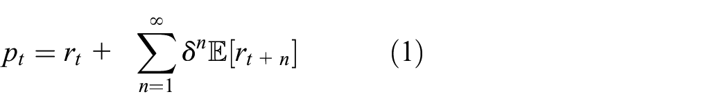
This equation captures the key insight we pull from asset valuation theory. If market participants begin expecting gentrification in several years, then landlords will anticipate being able to raise future asking rents by more than otherwise, while owner-occupiers anticipate an increase in their resale value.⁴ They will incorporate this into their willingness to pay, causing expectations of gentrification to directly increase the value of property today, and the price at which informed market participants expect it to transact.

This insight rests on a few features of market participants. First, participants must have (some, imperfect) knowledge about the gentrification status and trajectory of the neighbourhood. Qualitative studies identify the quite detailed insights residents have about change within their neighbourhood. This knowledge may take a spatial form, with a tacit understanding of which neighbourhood is next based on proximity to past gentrification and proximity to natural amenities or transportation infrastructure (e.g. Brown-Saracino, 2009: 58). Second, participant knowledge, however imperfect, needs to inform their actions (again, Brown-Saracino, 2009: 58). Third, it is not necessary that gentrification expectations be the key determinant of property values, only that they are sufficient to alter the value of property, all else equal.⁵

Given the US context, we use neighbourhood-level house values as our expectations-based variable and income as our present-oriented variable; both are available annually for small geographies. The signal could be improved by incorporating additional expectations-based variables beyond house values, or it could be modified to adapt to data availability in other countries – such as multifamily property values, physical investment, property tax valuation or comprehensive plans – and additional present-oriented measures like race or housing conditions.

To compare these variables, we convert neighbourhood-level average house values and incomes into relative percentile-ranks within a metropolitan area: the neighbourhood with the highest house prices will be around 1, and that with the lowest will be around 0. In general, the percentile-ranks of house prices and income are highly correlated, with the most expensive places also among the richest. For gentrifying neighbourhoods, we expect the house price percentile to be greater than the income percentile.

Figure 1 presents a stylised version of house value (solid) and income (dashed) percentile-ranks across three hypothetical neighbourhoods: one rich (dark/blue), one poor (light/green), and one that gentrifies during the period (medium/orange). The dark/blue lines cluster at the top of the city’s distribution for both house value and income percentiles while the light/green lines cluster near the bottom. The medium/orange lines begin near the bottom but, over time, market participants begin to expect gentrification. House values rise first, with the newly-opened gap between them signalling expectations of future gentrification.⁶ After several years, expectations become reality, and incomes rise too. Eventually, house values level off at a high level, while income growth continues.

Figure 1.

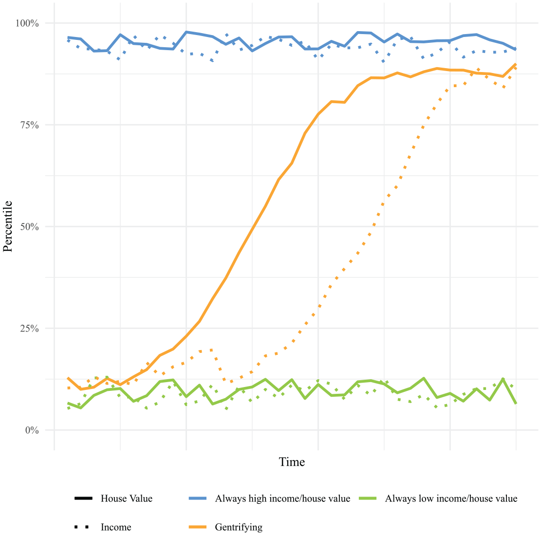
Conceptual example of house value and income percentiles in gentrifying and non-gentrifying neighbourhoods.

Measuring gentrification: Relative income and house prices

In this section, we summarise construction of our signal and the dynamic difference-in-difference regression model.⁷ For the signal, we use the smallest geographies – the census tract and ZIP code – with relatively frequent data releases. We use home price data from the Federal Housing Finance Agency (FHFA) House Price Index and income data from the Internal Revenue Service (IRS) Statistics of Income. Given limitations of the FHFA, we also construct our measure using the Zillow Home Value Index (ZHVI). We rely on census and American Community Survey (ACS) data, provided by the National Historical Geographic Information System (NHGIS) database (Manson et al., 2021). We examine historical gentrification using reweighted census data from Lee and Lin (2018) for census years from 1940 onwards, harmonised to 2010 census tract boundaries.

FHFA provides an annual estimate of changes to single-family house values relative to the prior year – it does not provide absolute values. At the tract and ZIP level, we reconstruct values for each geography in each year by multiplying the relative changes from FHFA by the median house value from the 2000 Census. In some contexts, it is more appropriate to use Zillow’s HVI at the ZIP level. The ZHVI provides black-box estimates of ‘typical’ house prices at the ZIP level, inclusive of single-family, condo and co-op typologies. We observe house prices from 1990 to 2020.

The IRS reports average income for each ZIP annually for 1998–2018. When doing an analysis at the spatial geography of the ZIP, we use the average household income constructed directly from the IRS data. At the tract level, we take the rate of year-over-year income change from the IRS for the ZIP in which the tract is located and multiply it by the median household income from the 2000 Census to estimate tract-level income for 1998–2018.

Next, we calculate the percentile-rank of each neighbourhood’s income and house values vis-à-vis the distribution of income and house values within its MSA. For every tract and ZIP within an MSA, we calculate the percentile rank of the house value, weighted by housing unit counts. For income, we weight by population.

To conduct statistical analyses, we construct a binary measure of gentrification for 1998–2018. Gentrifiable neighbourhoods are those in the inner third of an MSA based on distance to the central business district (CBD) with an initial income below the 25th percentile. These thresholds follow the gentrification literature in defining ‘gentrifiable’ areas (Finio, 2021). A neighbourhood is classified as gentrifying when a 25-percentile gap opens between the house values and incomes. This threshold balances competing risks: a low threshold could be triggered by short-term fluctuations; a high threshold may never be triggered – especially in neighbourhoods with little rental or social housing, where rising prices directly exclude new low-income buyers. In the qualitative comparison section, we highlight these trade-offs by exploring alternative thresholds.

To test whether a gap predicts future income growth in a neighbourhood, we use a dynamic difference-in-difference design (Sun and Abraham, 2021).⁸ We ask whether a house price/income gap in central low-income neighbourhoods is associated with future income growth, and how income growth depends on neighbourhood characteristics. Because we wish to include neighbourhoods with few single-family homes, we use ZHVI data at the ZIP code level. Out of 3329 centrally-located ZIPs, we identify 213 newly-gentrifying ZIPs between 1999 and 2018, and 97 already-gentrifying ZIPs. Our baseline estimating equation is:

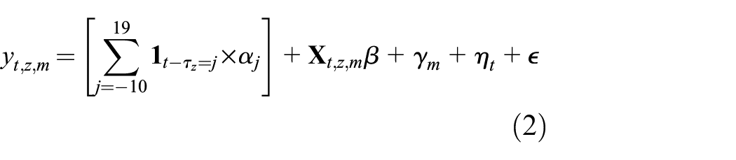
y_{t, z, m} = [\sum_{j = - 10}^{19} 1_{t - τ_{z} = j} \times α_{j}] + X_{t, z, m} β + γ_{m} + η_{t} + ϵ

(2)

Our dependent variable of interest, $y_{t, z, m}$ , is the log of the average income of ZIP z in year t in MSA m. The variable $τ_{z}$ is the year the ZIP first has a 25-percentile gap between house values and incomes. The variable [ $1_{t - τ_{z} = j}]$ is an indicator variable that equals 1 if a neighbourhood in year t is j years away from $τ_{z}$ , and 0 otherwise. All non-gentrifying neighbourhoods take a value of 0, as do already-gentrifying neighbourhoods for which a gap opened before the start of our data. Our main coefficient of interest is $α_{j}$ , which represents the relative income growth, in log-points, before or after gentrification onset in gentrifying neighbourhoods. We include a vector of control variables, $X_{t, z, m}$ : the log of neighbourhood income in 1998, pre-1998 gentrification status, neighbourhood socio-economic variables (from NHGIS), natural amenities (from Lee and Lin, 2018) and employment characteristics (from Manduca, 2020). The variables $γ_{m}$ and $η_{t}$ are MSA and year fixed effects, respectively.

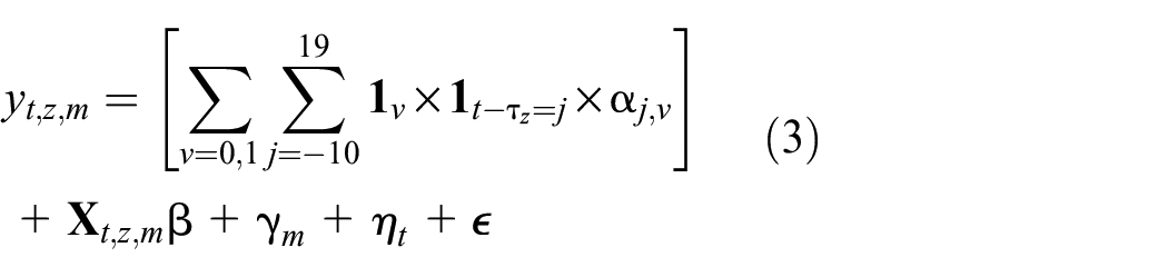
To test whether gentrifying neighbourhoods experience income growth differently depending on neighbourhood characteristics, we run additional regressions using equation (3). We interact gentrification status [ $1_{t - τ_{z} = j}]$ with another binary variable, $1_{v}$ , where a neighbourhood is either above (1) or below (0) a threshold for the variable of interest. The variables of interest selected for comparison are: share of the neighbourhood that is Black; the relative change in units in the neighbourhood between 2017 and 2000; and the distance to the CBD. For example, $1_{v} = 1$ if the neighbourhood is in the inner sixth of the MSA. These variables were chosen because of their relevance to threads in the literature: how gentrification is shaped by racialisation, new construction and centrality (Davidson and Lees, 2005; Rucks-Ahidiana, 2021; Smith, 1979).

\begin{matrix} y_{t, z, m} = [\sum_{v = 0, 1} \sum_{j = - 10}^{19} 1_{v} \times 1_{t - τ_{z} = j} \times α_{j, v}] \\ + X_{t, z, m} β + γ_{m} + η_{t} + ϵ \end{matrix}

(3)

Gentrification, neighbourhood context and income growth

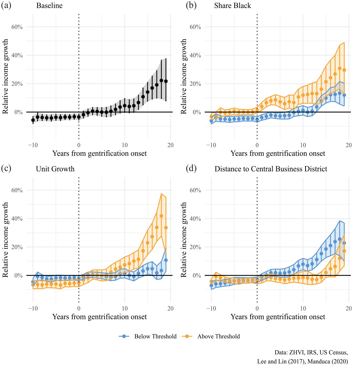
Figure 2 plots the estimates for $α$ , obtained from our regression models, and re-expressed as percentage growth in average neighbourhood income in the years before (to the left of 0) and after (to the right) a 25-percentile gap opens. These models control for the covariates described in the previous section. The shaded areas show the confidence intervals in the estimated income changes over time.

Figure 2.

Effect of a 25-percentile gap between house values and incomes.

Panel (a) of Figure 2 shows the baseline results of equation (2). Fifteen years after a gap opening, average income growth is 14% higher than would have been expected without a gap opening. This reflects rapid changes in neighbourhood composition in the years following gap opening – for comparison, US median household income grew 5% from 1998 to 2018 (U.S. Census Bureau, 2022). In contrast, panel (a) shows relatively little change in income prior to gap opening: income growth is slightly negative, but the estimates are stable rather than trending upward – which would indicate our measure is ‘too late’.⁹

The other panels present estimates of equation (3), comparing income trajectories among gentrifying neighbourhoods with different characteristics. Panel (b) shows that majority-Black neighbourhoods see rapid and sustained income growth after gentrification onset, while others see slower income growth. Prior to gentrification onset, majority non-Black neighbourhoods experience relatively low average income growth, matching the baseline figure but distinct from the experience of majority-Black neighbourhoods. These dynamics contrast somewhat with the findings of Rucks-Ahidiana (2021), who finds increases in higher-educated and White residents – but not high earners – in majority-Black gentrifying neighbourhoods. The different findings may be accounted for by differences in the time period under study, the gentrification measure or the measure of income changes.

Panel (c) shows that neighbourhoods with more housing growth experience greater income growth in the years following gentrification onset. This may reflect a few possible channels, among which our approach cannot distinguish: new construction may attract high earners, an influx of high earners may attract new construction, and the poor may be displaced through the construction process. This finding connects to Leguizamon and Christafore (2021), who show that neighbourhoods in development-constrained cities are somewhat less likely to gentrify. Because panel (c) shows income growth among neighbourhoods that do gentrify, our finding is compatible with theirs.

Panel (d) reveals that gentrifying neighbourhoods close to the CBD saw faster income growth, while neighbourhoods further out saw no faster growth upon gentrification onset. Fifteen years after a gap opens, neighbourhoods close to the CBD saw nearly 20% faster income growth, compared to essentially flat income growth in gentrifying neighbourhoods further from downtown. Centrality helps shape gentrification (Smith, 1979).

Collectively, these findings validate using house prices as an expectations-based signal for evaluating the onset of gentrification. The relationship between gap opening and income growth is mediated by other neighbourhood attributes: income growth follows more quickly among neighbourhoods that are closer to downtown, adding homes faster, and (initially) majority Black.

Validation: Qualitative and quantitative comparisons

In this section, we apply the signal to Boston and Chicago and compare our measure with extant qualitative studies in these cities using (variously) participatory, archival, ethnographic and interview methods to establish gentrification status. We view systematic qualitative investigation as the most appropriate benchmark for validating a gentrification measure. While we do not conduct our own qualitative work, our investigation of ‘neighbourhoods that qualitative researchers often highlight’ responds to calls to ‘bridge methodological divides’ (Brown-Saracino, 2016) by benchmarking our quantitative signal against qualitative insights. We also compare our measure to two established quantitative measures, both of which were focused on planning applications: Bates (2013), whose work was used in Portland’s comprehensive planning process (Bureau of Planning and Sustainability, 2018), and Los Angeles’s Index of Displacement Pressure, created by the Office of the Mayor’s Innovation Team (Pudlin, 2018).

Boston region

Binet (2021) uses survey and longitudinal interview methodologies within a participatory action research (PAR) process to study how gentrification affects caregiving relationships for residents in nine Boston-area neighbourhoods. Binet collaborated with resident researchers from these neighbourhoods to jointly develop hypotheses, research instruments and analyses of the resulting data. The study selected sites based on four criteria: having a walkable urban centre, a need for economic growth, early/mid-stage transformation and significant population health challenges (Binet, 2021: 48). After identifying three such sites with major health equity-oriented development projects planned, each was paired with two comparable sites without such plans. These criteria ruled out the South End, a traditional site of gentrification research in Boston, instead targeting neighbourhoods that began gentrifying more recently (e.g. Roxbury) as well as those that are experiencing other modalities of development (e.g. Brockton). We view the multi-site comparative nature of the study – including neighbourhoods in Boston proper, immediately adjacent communities, and more outlying places – as very useful for establishing a contemporaneous baseline of comparison to our quantitative signal.

In some neighbourhoods – Roxbury, Dorchester, especially, as well as Mattapan and the nearby small cities of Chelsea and Everett – residents described strong community ties and social support coupled with threats to stability from new development priced beyond their reach and new businesses that did not serve their needs. In contrast, residents of Brockton were as likely to describe the lack of investment, services and social connections as major challenges – features common in other outlying places in the study. Based on their analyses, we expect to see strong signals of gentrification in the core neighbourhoods of Roxbury and Dorchester as well as Mattapan, Chelsea and Everett, but not in Brockton.

Figure 3 applies our signal to these neighbourhoods using our ZIP dataset. Brockton is the clear outlier: house prices and incomes remain among the lowest in the MSA. By contrast, gaps have opened in every neighbourhood in which residents describe development pressures as a threat to caregiving responsibilities, with larger (and earlier) gaps in Roxbury and Dorchester. Our method provides a quantitative signal of the local knowledge Binet captures through PAR-based surveys and interviews. Using contemporaneous data, we see what is happening on the ground shortly after it takes place.¹⁰ However, our MSA-based operationalisation misses two places in Binet’s study that lie in southern Massachusetts, beyond the borders of the Boston MSA. Those places could be included by recalculating the percentiles inclusive of this area, reflecting the necessity of accounting for boundary effects.

Figure 3.

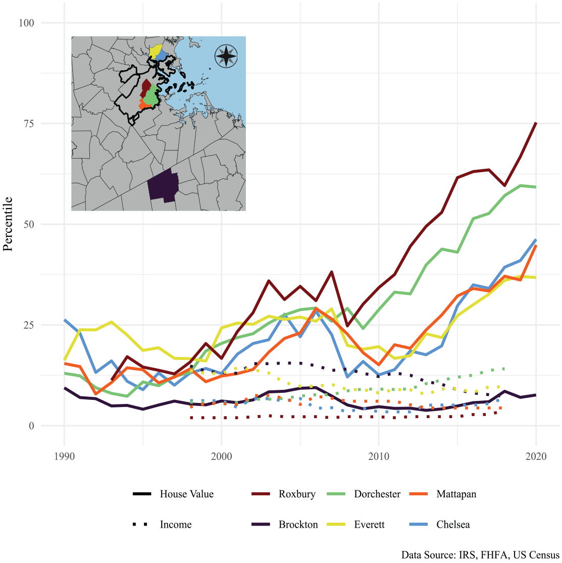
Greater Boston gentrification.

Chicago

In this subsection, we apply a threshold-based signal to study the history of gentrification in Chicago and compare our findings to the qualitative work of Perez (2004), Pattillo (2008), Hyra (2008), Brown-Saracino (2009) and Hertz (2018). Figure 4 maps the first year a gap opens between house value and income percentiles, using data from 1940 to 2019. To show the flexibility of our measure, we present two binary thresholds: a 20-percentile gap on the left panel and a 30-percentile gap on the right. We use two alternative neighbourhood definitions: the top panels use census tracts while the bottom panels aggregate tracts into city-defined community areas. Some tracts are missing price/income data in some years. For community areas, we only show results in years where data is reported for over three-quarters of the population.

Figure 4.

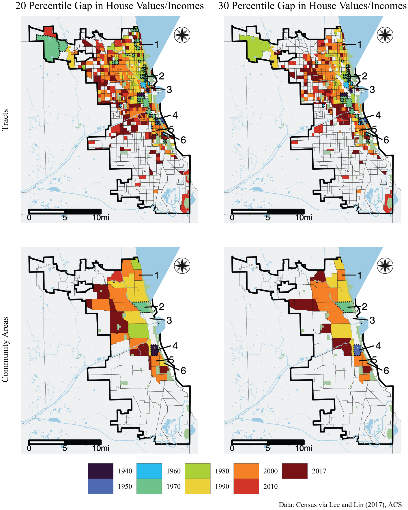
Gentrification in Chicago since 1940.

Figure 4 enables a cartographic reading of Chicago’s history of gentrification. Old Town was an early exemplar of gentrification (Hertz, 2018). The neighbourhood at its commercial heart saw gentrification as early as 1960. By the early 1970s, rising rents had pushed the bohemians north towards Lincoln Park where extensive gentrification throughout the community area is recorded as of 1970. Parts of Lincoln Park still had gaps open in recent decades despite having incomes well above the median, suggesting advanced gentrification.

Farther north, Edgewater is shown as gentrifying by 2000. Looking to its constituent census tracts, we can see substantial heterogeneity. Gaps opened in the sub-neighbourhoods of Andersonville during the 1980s and 1990s and Argyle by 1990 or 2000, in line with Brown-Saracino (2009). West and southwest of Lincoln Park, Puerto Rican and Ukrainian neighbourhoods show as gentrifying by 1990 or 2000, consistent with Perez (2004).

Pattillo (2008) and Hyra (2008) document gentrification in 1990s Kenwood/Oakland and Bronzeville, respectively. Unlike the north and northwest-side neighbourhoods discussed above, these Southside neighbourhoods were home to mostly Black residents at the onset of the processes, and Pattillo’s book documents a process of Black gentrification. In the context of racialised housing markets, gentrification may not generate expectations of rapid house price appreciation in Black neighbourhoods. In our maps, a single tract of Kenwood is gentrifying by 1990, and the community areas cross the 20-percentile threshold by 2000. Two Bronzeville tracts are shown as gentrifying by 1990, and more cross the threshold by 2000. Despite the different nature of gentrification in Black neighbourhoods, the signal works: the house price/income gap is significant in several tracts and opens in line with the processes described in their work.

However, the Douglas community area – overlapping Bronzeville – registers as gentrifying by 1940 or 1950. Douglas was not gentrifying in the 1940s; it was the core of the intensively segregated Black South Side. Why was there a gap? Intense segregation may have been directly responsible: the limited supply of housing available to Black families pushed prices up while labour-market segregation held down Black workers’ earnings (Boustan, 2016). The Douglas example emphasises the importance of combining any metric with local knowledge, and the simplicity of doing so with our metric.

Comparing across panels reveals trade-offs of using different neighbourhood boundaries and gap thresholds. Community areas are larger than the neighbourhoods qualitative researchers generally study, and mask substantial variation across tracts. At the same time, some spatial variation is statistical noise, which aggregating smooths. The 20-percentile threshold results in a very advanced gentrification frontier in recent years. By contrast, the larger threshold misses some places with rising incomes and house prices that never see a 30-percentile gap – including many surrounded by gentrifying places. These tensions are inherent to quantitative measurement, and our signal cannot avoid them. Our use of a 25-percentile threshold elsewhere in the paper aims to balance these competing risks.

Portland

Bates (2013) studies gentrification in Portland, Oregon, between 1990 and 2010. She draws definitional characteristics from Freeman (2005), and her approach has been taken up since, for example, by Chapple et al. (2022), thus offering a practice-engaged and academically-representative example of quantitative gentrification measurement. Bates classifies tracts based on the presence of a ‘vulnerable’ population, housing market factors, and demographic change. (Most tracts lack these features and were coded NA.)

Figure 5 presents our measure for Portland tracts during the period 1998–2018, with separate panels for each of Bates’s tract types. For clarity, we bold low-income tracts after a 25-percentile gap has opened. Our measures largely agree. Many tracts undergoing ‘early’ gentrification see sizeable house value/income gaps open, and tracts classified as ‘Dynamic’, ‘Late’ or ‘Continued Loss’, have rapidly rising house prices with trailing, but increasing, incomes. However, our measure picks up likely gentrification Bates’s approach misses. The dark bolded tract in the ‘NA Tract, High Vulnerability’ panel appears to be experiencing post-industrial gentrification: house values increased from near the median to the top quartile by 2003, while incomes increased from the 3rd to the 15th percentile by 2018.

Figure 5.

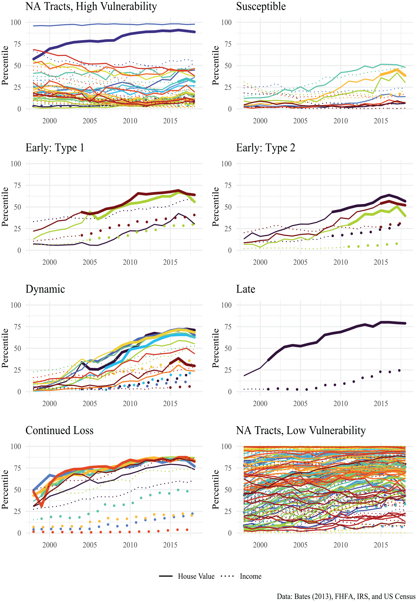
Gentrification in Portland, comparing the Bates (2013) findings to our measure.

There is overall alignment between neighbourhoods Bates classifies as undergoing gentrification, and those tracts where we see rising house values and lagging (but rising) incomes. Against a popular quantitative measure of gentrification, our measure performs similarly.

Los Angeles

The Los Angeles Innovation Team developed the Los Angeles Index of Displacement Pressure (LAIDP) to map gentrification and influence planning (Pudlin, 2018). This prospective measure identifies neighbourhoods with future displacement risks by integrating the Los Angeles Index of Neighbourhood Change (Pudlin, 2016) – a retrospective index akin to Bates (2013)– with displacement risk factors: expiring affordable housing units, transit facilities, rental market factors and a proprietary forecast of house price growth from Esri.

Figure 6 maps the LAIDP (top left) and the house value/income gap in five-year increments for 1998–2018 for LA ZIPs (other panels). The city borders are outlined with a thin black line. There is substantial concordance between the approaches. Very high- and high-risk areas in Central LA have sizeable gaps, while smaller gaps are visible in South and Northeast LA that are medium risk in the LAIDP. Areas in the distant edges of the San Fernando Valley have modest negative gaps and are largely classed as low risk by the LAIDP. Differences arise in the large gaps of late-stage gentrifying neighbourhoods like Venice Beach and in college-adjacent areas like University Park, labelled low risk in the LAIDP. Further, the LAIDP shows higher risks in other parts of downtown than our measure. This reflects extremely rapid income growth downtown, surpassing the median and closing the gap by 2010. The displacement risk warned of by the LAIDP was already visible in the rearview mirror.

Figure 6.

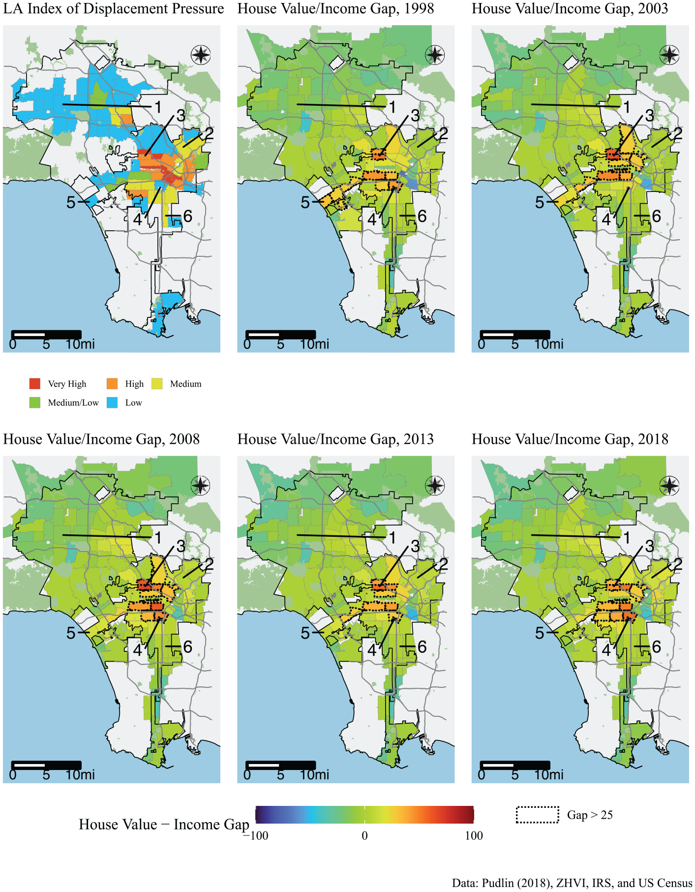
Los Angeles index of displacement pressure and house value/income gap over time.

Mapping the gap over time offers some unique insights. Changes across panels are subtle – and for much of the city, the panels are nearly identical (and the gaps are near zero). These subtleties reveal variation in how far in advance house values anticipate future projected displacement risk: Central LA has large gaps open by 1998, while Northeast LA only sees a gap open more recently. Relative to the maps of Chicago, this approach reveals gaps closing, as in Venice Beach, a (now) wealthy coastal enclave. For gentrifying places, a constant gap does not imply stasis in the neighbourhood measured; instead it could reflect rising house values and incomes.

An expectations-based signal improves understanding

In this paper, we developed an expectations-based measure of gentrification. Asset valuation theory shows that property values incorporate the expectations of market participants. We use this theory to interpret property values as incorporating local market participant knowledge about a neighbourhood’s future. If their expectations are correct, the future holds rising incomes, capital investment, landscape change, displacement and other changes characterising gentrification.

We operationalise this insight by comparing the percentile-rank of a neighbourhood’s house prices and incomes. In the US, these components are released on at least an annual basis, enabling rapid identification of expected gentrification. We interpret a sizeable gap between the two as a signal of gentrification. Using annual data and a dynamic difference-in-difference framework, we demonstrate that incomes rise rapidly following the opening of a substantial gap. Our signal overlaps empirically with existing measures of gentrification and improves upon them by offering easy application to time-series, cross-sectional and panel contexts. The signal can be plotted over time (as we demonstrate for Boston and Portland) and mapped cross-sectionally (as for Los Angeles) or by mapping gentrification’s path through a city over time (as for Chicago).

We note several limitations. Our emphasis on the convenience of house prices and incomes costs us nuance. House prices may proxy poorly for property values in areas with mostly rental or social housing. We may miss marginal gentrification that does not translate immediately into house prices, as well as interventions like state-led gentrification. In these cases, house prices may be a lagging indicator. Other variables incorporating expectations of the future include multifamily property values, investment decisions and city plans. Income does not fully characterise vulnerability to gentrification, and without including (e.g.) a direct racial component, we may misstate risks. Our percentile-based measure may flatten meaningful differences. Brooklyn Heights, in the period Lees (2003) studies, has a small house value/income gap, but the fractal nature of top income inequality means ‘super-gentrification’ may nevertheless push house prices beyond the reach of the merely rich. In the analysis shown in Figure 2, we only test income growth, not other relevant outcomes. Empirically, we identify some neighbourhoods as gentrifying that do not have established records of research, raising the possibility of false positives.

Set against these limitations are the significant benefits of a timely, well-understood and readily-available measure of gentrification. Our approach can be used by practitioners and researchers alike to track gentrification at the local level. Practitioners implementing policies to mitigate negative effects of gentrification can only do so if they have accurate, timely measures of on-the-ground changes. Our signal meets those needs, while providing interpretability and flexibility allowing for its deployment in planning contexts. For researchers, the annual signal and difference-in-difference implementation offer a new way of studying diverse outcomes in gentrifying places (e.g. Kavanagh-Smith, 2021). Beyond the gap, plotting house price and income percentiles over time offers insight into gentrification by revealing how a gentrifying neighbourhood has moved through its city’s socio-economic hierarchies – even in cases where a gap does not open. Our conceptual distinction of expectations-based variables offers a new approach to identifying gentrification, and we hope further variables can be brought into this framework.

Supplemental Material

sj-docx-1-usj-10.1177_00420980231173846 – Supplemental material for Re-measuring gentrification

Supplemental material, sj-docx-1-usj-10.1177_00420980231173846 for Re-measuring gentrification by devin michelle bunten, Benjamin Preis and Shifrah Aron-Dine in Urban Studies

Footnotes

Acknowledgements

We are deeply indebted to the research assistance of Madeleine Daepp (for her exceedingly thorough and diligent data analysis) and Emily Moss (for her support in tracking the literature and copy editing). We are grateful to insightful comments from an array of readers, including Vicki Been, Japonica Brown-Saracino, Mike Lens, Paavo Monkkonen and Justin Steil. We are also grateful to countless seminar and conference attendees for thoughtful questions and comments, as well as to many readers of earlier iterations of this paper.

Declaration of conflicting interests

The author(s) declared no potential conflicts of interest with respect to the research, authorship, and/or publication of this article.

Funding

The author(s) disclosed receipt of the following financial support for the research, authorship, and/or publication of this article: This paper draws in part on work supported by the National Science Foundation Graduate Research Fellowship under Grant No. DGE-1745302. Any opinions, findings and conclusions or recommendations expressed in this material are those of the authors and do not necessarily reflect the views of the National Science Foundation.

ORCID iDs

devin michelle bunten

Benjamin Preis

Supplemental material

Supplemental material for this article is available online.

Notes

References

Barton

(2016) An exploration of the importance of the strategy used to identify gentrification. Urban Studies 53(1): 92–111.

Bates

(2013) Gentrification and displacement study: Implementing an equitable inclusive development strategy in the context of gentrification. Working Paper, Urban Studies and Planning Faculty Publications and Presentations, Portland State University.

Beauregard

(1986) The chaos and complexity of gentrification. In: Smith

Williams

(eds) Gentrification of the City. London: Routledge, pp.35–55.

Binet

(2021) Making the city livable: Caregiving and health in gentrifying Boston. Dissertation, Massachusetts Institute of Technology. Available at: https://hdl.handle.net/1721.1/140051 (accessed 20 February 2023).

Boustan

(2016) Competition in the Promised Land: Black Migrants in Northern Cities and Labor Markets. Princeton University Press. Available at: https://www.nber.org/books-and-chapters/competition-promised-land-black-migrants-northern-cities-and-labor-markets (accessed 18 December 2021).

Brown-Saracino

(2009) A Neighborhood That Never Changes. Fieldwork Encounters and Discoveries. Chicago, IL: The University of Chicago Press.

Brown-Saracino

(2013) The Gentrification Debates. London: Routledge.

Brown-Saracino

(2016) An agenda for the next decade of gentrification scholarship. City and Community 15(3): 220–225.

Brown-Saracino

(2017) Explicating divided approaches to gentrification and growing income inequality. Annual Review of Sociology 43(1): 515–539.

10.

Bureau of Planning and Sustainability (2018) 2035 Comprehensive Plan. December. City of Portland. Available at: https://www.portlandoregon.gov/bps/2035-comp-plan.pdf (accessed 18 December 2022)

11.

Chapple

Poorthuis

Zook

, et al. (2022) Monitoring streets through tweets: Using user-generated geographic information to predict gentrification and displacement. Environment and Planning B: Urban Analytics and City Science 49: 704–721.

12.

Davidson

Lees

(2005) New-build ‘gentrification’ and London’s riverside renaissance. Environment and Planning A: Economy and Space 37(7): 1165–1190.

13.

Department of Neighborhood Development (2021) Income Restricted Housing in Boston 2020. City of Boston. Available at: https://www.boston.gov/sites/default/files/file/2021/03/Income%20Restricted%20Housing%202020_0.pdf (accessed 19 January 2023).

14.

Easton

Lees

Hubbard

, et al. (2020) Measuring and mapping displacement: The problem of quantification in the battle against gentrification. Urban Studies 57(2): 286–306.

15.

Ellen

O’Regan

(2011) How low income neighborhoods change: Entry, exit, and enhancement. Regional Science and Urban Economics 41(2): 89–97.

16.

Finio

(2021) Measurement and definition of gentrification in urban studies and planning. Journal of Planning Literature 37: 249–264.

17.

Fisher

(1906) The Nature of Capital and Income. New York, NY: The Macmillan Company.

18.

Fonner

Izón

Feist

, et al. (2022) Capitalization of reduced flood risk into housing values following a floodplain restoration investment. Journal of Environmental Economics and Policy. Epub ahead of print 3 November 2022. DOI: 10.1080/21606544.2022.2136765.

19.

Freeman

(2005) Displacement or succession?: Residential mobility in gentrifying neighborhoods. Urban Affairs Review 40(4): 463–491.

20.

Galster

Peacock

(1986) Urban gentrification: Evaluating alternative indicators. Social Indicators Research 18(3): 321–337.

21.

Glaeser

Kim

Luca

(2018) Nowcasting gentrification: Using yelp data to quantify neighborhood change. AEA Papers and Proceedings 108: 77–82.

22.

Glickman

(2014) Property valuation. In: An Introduction to Real Estate Finance. Amsterdam: Elsevier, pp.129–151.

23.

Goetz

Lewis

Damiano

, et al. (2019) The diversity of gentrification: Multiple forms of gentrification in Minneapolis and St. Paul. Center for Urban and Regional Affairs, University of Minnesota. Available at: https://gentrification.umn.edu/sites/gentrification.umn.edu/files/files/media/diversity-of-gentrification-012519.pdf (accessed 13 February 2022).

24.

Golub

Guhathakurta

Sollapuram

(2012) Spatial and temporal capitalization effects of light rail in Phoenix: From conception, planning, and construction to operation. Journal of Planning Education and Research 32(4): 415–429.

25.

Hammel

Wyly

(1996) A model for identifying gentrified areas with census data. Urban Geography 17(3): 248–268.

26.

Hertz

(2018) The Battle of Lincoln Park: Urban Renewal and Gentrification in Chicago. Cleveland, OH: Belt Publishing.

27.

Hwang

Shrimali

(2021) Constrained choices: Gentrification, housing affordability, and residential instability in the San Francisco Bay Area. Community Development Research Brief 2021–2, Federal Reserve Bank of San Francisco. Available at: https://www.doi.org/10.24148/cdrb2021-02 (accessed 13 February 2022).

28.

Hyra

(2008) The New Urban Renewal: The Economic Transformation of Harlem and Bronzeville. Chicago, IL: University of Chicago Press.

29.

Jain

Proserpio

Quattrone

, et al. (2021) Nowcasting gentrification using Airbnb Data. Proceedings of the ACM on Human-Computer Interaction 5(CSCW1): 1–21.

30.

Kaplan

Mitman

Violante

(2020) The housing boom and bust: Model meets evidence. Journal of Political Economy 128(9): 3285–3345.

31.

Kavanagh-Smith

(2021) Does gentrification contribute to homelessness? A study of family shelter entry across New York City, 2005–2015. Dissertation, The New School, New York. Available at: https://www.proquest.com/pagepdf/2557509612?accountid=12492 (accessed 26 January 2023).

32.

Lee

Lin

(2018) Natural amenities, neighbourhood dynamics, and persistence in the spatial distribution of income. The Review of Economic Studies 85(1): 663–694.

33.

Lees

(2003) Super-gentrification: The case of Brooklyn Heights, New York City. Urban Studies 40(12): 2487–2509.

34.

Leguizamon

Christafore

(2021) The influence of land use regulation on the probability that low-income neighbourhoods will gentrify. Urban Studies 58(5): 993–1013.

35.

Liu

Deng

Song

, et al. (2019) A comparison of the approaches for gentrification identification. Cities 95: 102482.

36.

Manduca

(2020) The spatial structure of US metropolitan employment: New insights from administrative data. Environment and Planning B: Urban Analytics and City Science 48(5): 1357–1372.

37.

Manson

Schroeder

Van Riper

, et al. (2021) National Historical Geographic Information System: Version 16.0. Minneapolis, MN: IPUMS.

38.

Pattillo

(2008) Black on the Block: The Politics of Race and Class in the City. Chicago, IL: University of Chicago Press.

39.

Perez

(2004) The Near Northwest Side Story: Migration, Displacement, and Puerto Rican Families. Berkeley, CA: University of California Press.

40.

Preis

Janakiraman

Bob

, et al. (2020) Mapping gentrification and displacement pressure: An exploration of four distinct methodologies. Urban Studies 58(2): 405–424.

41.

Pudlin

(2016) Los Angeles index of neighborhood change. City of Los Angeles Open Data. Available at: http://geohub.lacity.org/datasets/57e9231c3bd34d44ae49b309b0cb440e_1 (accessed 21 May 2019).

42.

Pudlin

(2018) Los Angeles index of displacement pressure. City of Los Angeles Open Data. Available at: http://geohub.lacity.org/datasets/70ed646893f642ddbca858c381471fa2_0 (accessed 21 May 2019).

43.

Reades

De Souza

Hubbard

(2019) Understanding urban gentrification through machine learning. Urban Studies 56: 922–942.

44.

Rucks-Ahidiana

(2021) Racial composition and trajectories of gentrification in the United States. Urban Studies 58(13): 2721–2741.

45.

Smith

(1979) Toward a theory of gentrification A back to the city movement by capital, not people. Journal of the American Planning Association 45(4): 538–548.

46.

Sun

Abraham

(2021) Estimating dynamic treatment effects in event studies with heterogeneous treatment effects. Journal of Econometrics 225(2): 175–199.

47.

U.S. Census Bureau (2022) Real median household income in the United States. FRED, Federal Reserve Bank of St. Louis. Available at: https://fred.stlouisfed.org/series/MEHOINUSA672N (accessed 13 February 2022).

48.

Zapatka

Beck

(2021) Does demand lead supply? Gentrifiers and developers in the sequence of gentrification, New York City 2009–2016. Urban Studies 58(11): 2348–2368.

Supplementary Material

Please find the following supplemental material available below.

For Open Access articles published under a Creative Commons License, all supplemental material carries the same license as the article it is associated with.

For non-Open Access articles published, all supplemental material carries a non-exclusive license, and permission requests for re-use of supplemental material or any part of supplemental material shall be sent directly to the copyright owner as specified in the copyright notice associated with the article.

0.00 MB

0.03 MB