
Abstract
The generation of ever-bigger data sets pertaining to the distribution of activities in cities is paralleled by massive increases in computer power and memory that are enabling very large-scale urban models to be constructed. Here we present an effort to extend traditional land use–transport interaction (LUTI) models to extensive spatial systems so that they are able to track increasingly wide repercussions on the location of population, employment and related distributions of spatial interactions. The prototype model framework we propose and implement called QUANT is available anywhere, at any time, at any place, and is open to any user. It is characterised as a set of web-based services within which simulation, visualisation and scenario generation are configured. We begin by presenting the core spatial interaction model built around the journey to work, and extend this to deal with many sectors. We detail the computational environment, with a focus on the size of the problem which is an application to a 8436 zone system comprising England, Scotland and Wales generating matrices of around 71 million cells. We detail the data and spatial system, showing how we extend the model to visualise spatial interactions as vector fields and accessibility indicators. We briefly demonstrate the implementation of the model and outline how we can generate the impact of changes in employment and changes in travel costs that enable transport modes to compete for travellers. We conclude by indicating that the power of the new framework consists of running hundreds of ‘what if?’ scenarios which let the user immediately evaluate their impacts and then evolve new and better ones.
Defining big, defining scale
Big data and computable urban models
The digital computer was invented in several places in the decade spanning the Second World War, and as soon as it emerged from its scientific and philosophical origins, it was applied to large-scale problems involving predicting human futures as well as accounting and transactions processing in business. The focus was on both solving problems that involved large-scale data as well as fast computation, and these foci have remained at the heart of computing ever since. ‘Big data’ and ‘big computation’ have gone hand in hand, and although big data tends to be in the ascendency today, large-scale computation is in fact equally important in that computation generates more data that becomes ever bigger. The data manipulated by Google in its search functions, for example, is far larger than the raw data itself, as every search initiated reuses and transforms raw data over and over again. It is thus the number of users and their continued interrogation of data that is big, not necessarily the data per se.
Urban models were first constructed in the late 1950s as simulations of land-use location and transportation flows. In this journal, Wilson (1968) reviewed the early experience of using these models in strategic planning, and four years later Batty (1972) followed this with a review of the nascent British experience. Computer models have always been problematic in terms of their development and use, up against the limits posed by inadequate theory, poor quality and missing data and computational memories that have constrained the size of the urban system represented. But limits posed by computation have massively relaxed as miniaturisation has continued apace, and it is now possible to operate quite big models on personal devices. Indeed, the modelling framework which is the focus of this article can be run on a smartphone, and in essence this means that computation is no longer a severe problem. The use of models as a key instrument of planning support has not changed much either during these years, for the notion of using them to evaluate strategic land-use and transportation policies in a ‘what if?’ manner still remains the goal of using them to inform predictions and explore scenarios for future cities.
The model framework proposed here is in fact different from most other previous applications in that the focus is on building spatially extensive urban land-use transportation models that can be run almost immediately, thus providing the user with rapid feedback with respect to the evaluation of scenarios. The reason for this rapidity is that the potential solution space for urban futures is enormous and has rarely been charted. We are moving to an era where hundreds if not thousands of solutions might be explored in much the same way as online search systems operate, enabling massive numbers of queries to be handled which can only be absorbed by users in real time. Although our model’s application is to spatially extensive ‘big’ data based on many spatial zones and detailed interaction patterns and networks, it is the operation of the model over and over again with the user evaluating alternative after alternative in ‘real time’, not waiting for hours or days to retrieve model runs and evaluate them in a more leisurely fashion, that is the innovation in the big data emphasised here. We do not have the space to explore the new methods of scenario generation in detail here which depend on structured learning in the solution space of possible futures; all we will attempt is to outline our new framework, making clear the way in which a user can interact with big data and big computation across a variety of dimensions. This will take the big data argument well beyond most of the discussions about big data per se which usually emanate from real-time streaming based on embedded sensor technologies.
The framework we will propose is essentially geared to gravitational-discrete choice models which are static simulations of urban structure at a single point in time. Other models reflecting agent-based representations could easily be slotted into this framework, but aggregate models of the kind proposed are much more suitable in that they perform far better than more disaggregate and temporally dynamic variants. These newer agent-based models take much longer to run, their data is more problematic and, in practice, they have a much poorer track record in terms of their validation, with the authors having a long experience in working with this entire variety of models as well as their embedding in the planning process (Batty, 2005, 2013).
The renaissance of large-scale modelling
The earliest urban models stretched the limits of computing and data in terms of the volume and type of data required and the computational resources available. Data in cities is spatially extensive, and can never be detailed enough in terms of how many different types of sector and population are characterised. Processing time is a function of the speed at which computation takes place, which in turn is a function of chip technology and the memory available for randomly accessing data. Yet despite these limits, computational speed and memory have increased exponentially, doubling every 18 months according to Moore’s Law. Many of the earliest critiques (see Lee, 1973) were devoted to how these computational problems limited the effectiveness of these early models, and although our theories of how cities work have remained quite rudimentary, our ability to construct such models and push them towards conditional prediction has improved immeasurably (Harris, 1994; Te Brömmelstroet et al., 2014). The models of yesteryear took months to construct and often days to run, while the same sized models today can be built in a matter of hours and run in minutes or, as we will see in this article, in a matter of seconds.
The quest to build larger urban models has thus revolved around disaggregation of activities, spatial units and temporal intervals to the finest categories possible, but the models that have emerged are no better, if not worse, in their applicability to planning. New models reflecting spatial units at the level of cells (cellular automata – CA models), individuals as agents (agent-based models – ABM) and microsimulation have emerged. Although there are an increasing variety of urban models, big data, much of it captured in real time, is not easy to link to LUTI, ABM, CA and microsimulation models. Social media data is a case in point, detecting behaviours that are not included in the kinds of urban model that have been developed over the last half century, and although such data may be rich in detail, it is usually unrepresentative, non-comprehensive and not easy to use as a proxy for the data required in urban simulation models. In the framework we develop in the rest of this article, we will outline the model first, extend it to a general form, describe how we develop it as a set of web services and then discuss its computational requirements. We outline the data required and then present ways in which it can be used for impact analysis through ‘what if?’ scenarios. We then just outline two typical scenarios from the hundreds that we could test, and conclude by emphasising once again that the power of the model lies in its potential to evaluate an unlimited number of urban futures that bound the solution space. First, however, we introduce the model’s notation.
Notational representation, extensive scale and intensive computation
All our variables are urban activities defined by their location, the time at which they are observed and the sector to which they belong. A generic activity is defined as
Without interactions, this might just be considered as ‘big data’, and there are plenty of examples where this number can be generated from data collected in traditional ways such as from Population Censuses. But the volume of data associated with this way of representing the urban system only begins to explode when interactions between urban activities are defined. We will define the interaction between urban activities with respect to their location in space and time as follows. Typically, we define a flow between activity at
Our models in this article will not focus on urban dynamics which explode these problems even further, but are models of urban flows at a cross section in time, and this means that we can drop the index
The generic urban equilibrium model
The core spatial interaction model
The large-scale urban model that we will introduce here has at its core the flow or interaction between different activities in different locations. The generic model predicts these flows as
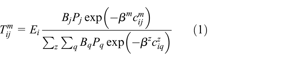
where
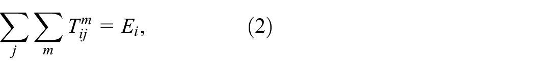
This model is constrained so that the trips over all modes sum to the employment at the origin
from which it is also clear that the modal split between any two modes
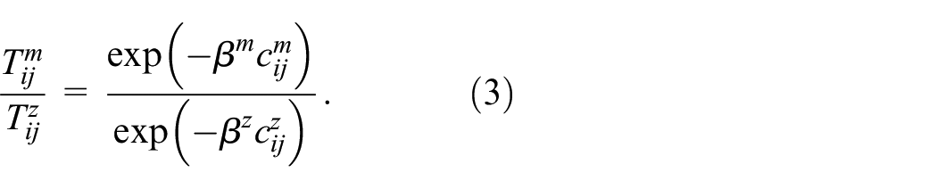
Equation (3) shows that the model simulates competition between the modes, enabling modal shifts to be predicted, which is an essential and rather innovative focus of the model.
If there are capacity constraints

where

The parameters
The simultaneity of activity allocation
So far, we have only introduced a single spatial interaction which can be interpreted as simulating the process where the demand by the working population at their place of employment is supplied at their place of residence. We can also consider the supply of residential population from their place of residence as generating a demand for employment at their place of employment. In short, we need to model demand from workplaces for residences and demand from residences for workplaces. This is the simultaneous nature of demand and supply of the working population where we need to simulate how the location of employment determines population and vice versa.
We will begin by stating the residential location model again from equation (1) above but now noting that we introduce a ‘temporal’ index
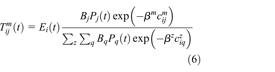
where
from which we can now generate a new estimate of employment
where
We are now in a position to start the iteration using
The advantage of this sequence is that the starting point can either be the observed data or it can be a prediction. In fact, a variant of this method is to collapse demand into supply and predict origin employment
Implementation of the model system
The model interface
There are many very large-scale urban models that have big data requirements, as well as computational processing times that make them highly unsuitable for any kind of interactive use. There has been a trend in this field to build ever more disaggregate models which require iterative balancing procedures that can take days to run on even the most powerful computers, although these limits are continually being extended. For example, the move from LUTI and four-stage transport model structures to ABM, as for example in UrbanSim (Waddell, 2002) and MATSim (Horni et al., 2016), makes their data requirements formidable, the time to perform one run of the model often prohibitive and the effort needed to support plan-making activities well beyond the resources of most agencies (Moeckel, 2018).
In the model proposed here, we set very strict limits on the extent of the spatial systems for which the model is to be built, the data required, the turnaround time for a model run and the accessibility of the system to many users. The model we are building is essentially a sketch planning tool to enable ‘what if?’ type impacts on the location of employment, population and transportation infrastructure to be evaluated. These impacts are spatially extensive, well beyond the local level, to regional and national scales and thus the relevant spatial system must capture as many of these spatial effects as possible. In this context, the model is to be applied to an entire country, that is, the island of Great Britain (England, Scotland and Wales), and this means that it is available to any municipality or regional or local authority for various kinds of physical planning. In short, the model needs to be able to trace the impacts of infrastructure changes such as national and regional high-speed rail lines, new motorway systems, airports, national parks policies, green belts, large-scale housing developments and so on.
The model also needs to be available to any user for any place within the country, at any location where the user is based and at any time. This implies that it should be free at the point of use and available in a medium that makes it immediately accessible, and this implies that it should have an open web interface. Moreover, it should be available on as many devices as possible, from a smartphone to a supercomputer, although generically our aim is to make it most robust for desktop/laptop use and the current version when viewed on a smartphone is not ideal. Although the model has been financed through research agencies making it free at the point of use, this does not mean that the model is open source as it has not (yet) been funded or designed to make this possible. As the model is highly user focused through its web interface, it needs to run rapidly and although the user might be engaged in other tasks, a single run beyond 30 seconds on any hardware which is based on GPU servers is not acceptable. Users require almost immediate feedback numerically and graphically and, to an extent, this will dictate the size of the model, the data and the methods of programming. Another criterion relates to the number of users. Currently, each user generates their own thread once they activate the model, and this means that we have to pay special attention to the relationship between the user’s client and the server side so that unacceptable queues composed of many users accessing the servers do not build up. Currently the model is a prototype and we do not anticipate there being more than a handful of users at any one time. Last but not least, the model interface needs to be user-friendly and its graphics meaningful, rich and visually attractive, so that users are drawn into using the system most effectively.
Although it is possible to make the model and data available as a downloadable package which an individual user might run on their own system, the size of data and the speed of processing are such that more powerful systems that take account of memories and computational processing power in server environments are necessary for the applications developed here. Moreover, the distribution of data and model is more easily accomplished through continual interaction between servers and clients, and because the type of the client is under the control of the user, it is not possible to ensure that the user always has a powerful enough client to run the entire application locally for the size of spatial system envisaged (such as England, Scotland and Wales). In fact, the system is articulated in three parts – a website, a mapping system reflecting the data and the model – with these resources distributed between server and client, in the ways we will indicate in the next section where we detail how the interface has been developed.
Urban modelling as a web service
Figure 1 shows the various computational processes involved in constructing the model, with a distinction made between web-based services and model computation largely constituting server-side functions, and visualisation focusing on client-side services. This is consistent with a system where we never know in advance what client the user has available to operate the framework.
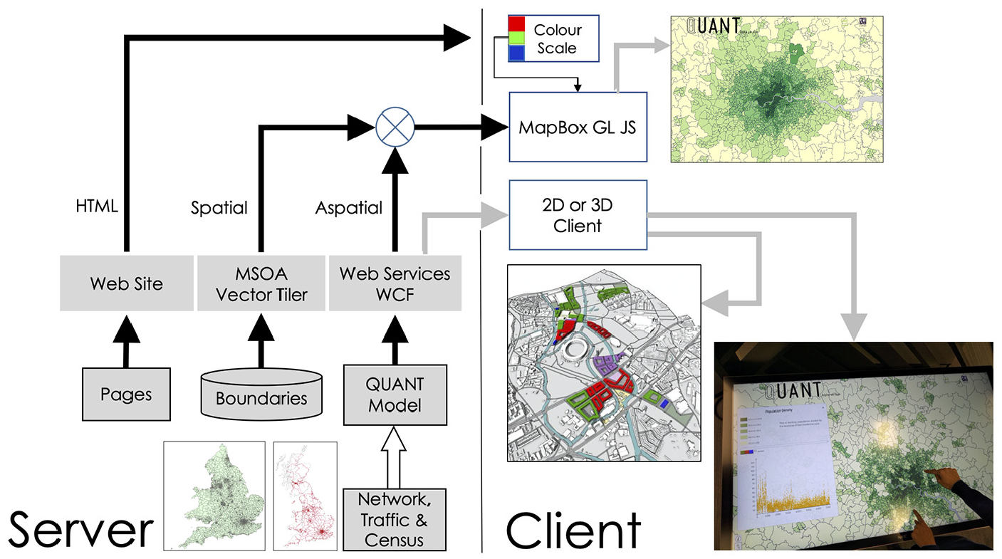
The computational environment: Organisation of the client–server environment, web services, data input, simulation and visualisation.
The model is called QUANT, which stands for Quantitative Urban ANalytics forecasTing or some variant thereof, and its underlying architecture is based on Microsoft.Net Core 3. This allows portability to other platforms, with the server-side web mapping (MSOA Vector Tiler) and the QUANT model being developed in C#. The website and its user interface use Angular 8 with NodeJS on the server side. The combination of .Net Core with NodeJS and Angular is a common design pattern which is geared towards developing complex Single Page Applications (SPA) such as those required to provide a web-based GIS with the capability to visualise the model outputs of QUANT immediately. If we take the model in equations (1) to (4), then each trip and cost matrix
Computational processing
Before we note the computational structure relevant to the model itself and its visualisation, we must note that by far the biggest computational burden involved in this type of model involves determining the matrix of shortest path costs that are essentially built from very detailed network representations of the three modes – road, bus and rail. The road network consists of some 8.401 million line segments and 3.527 million nodes, the bus network of some 1.980 million segments and 332,720 nodes and the rail network, which is by far the sparsest, of some 9254 segments and 2595 nodes. We need to define zone centroids and compute the shortest paths using these networks which link all pairs of the 8436 zones, and this generates the relevant cost matrices, each of dimension 71 million cells, which are basic inputs to the models shown above. Now, as the framework is designed to enable users to build scenarios on the fly within the model interface and to run the model and evaluate impacts of the scenario on the entire spatial system in real time, these shortest route problems need to be solved within the model framework itself. In fact, so far this is only possible for the rail network, so to operate the model in the first instance the shortest paths must be pre-processed and fed into the model as input data.
Running an All Pairs Shortest Path (APSP) algorithm for all pairs of street nodes takes over two hours for a full calculation of the road costs, but this comes down to only one minute for the rail network, due to relative sparsity of edges and nodes. This is still too slow, and at present the framework only offers rail network modification on the website using an approximate method to further improve the speed of the travel time matrix calculations. We are currently investigating a variety of approximations to compute these shortest paths in real time, that is, as the user is running the model, but this requires several new methods that are currently under development, notwithstanding that fast solutions to the shortest route problem as originally posed and solved by Dijkstra (1959) have been very slow in forthcoming.
Various elements of the model computation can be speeded up, and if we examine equation (1) again it is clear that it can be written in matrix terms as
Before we examine the data and the spatial system that the model is designed to simulate, we need to detail the client-side operations that pertain to visualisation. The model front end relies on Angular 8 and a NodeJS server running in parallel with ASP.net MVC and .Net Core 3.0. This allows the client side to act as a model view controller, where the model is being controlled by the Javascript Angular 8 front end on the web page. Aside from the navigation pages on the website, two of the pages display maps and data to the user, with the scenario page additionally allowing the QUANT model to be re-run with user-specified scenario data. We will show some of these operations in the implementation and applications below, but the basic maps page and the scenario page are actually the same Angular component, just with the addition of the scenario controller component on the scenario page. The underlying map uses MapBox GL JS to display a choropleth map of England, Scotland and Wales at the resolution of the middle layer superoutput area (MSOA), which is one of the standard small-area UK geographies for spatial analysis at the level of city regions. The ASP.net server acts as the tile server, delivering MapBox tiles to the client when requested. This runs outside of the NodeJS and Angular framework, with the requests going directly to the IIS (Internet Information Server). These tiles are served blank, without any data bound to them, as every user on the system is viewing a different map or a different scenario, and this architecture allows maximum use of tile caching. Users viewing maps, or scenario runs, in the web interface request data specific to them via the model’s web services framework, which delivers a set of key/value pairs where the key is the area code for the MSOA region and the value might be population density, or results from a scenario run. This data is bound to the map on the web page using MapBox GJ JS, thereby decoupling the spatial part of the GIS system from the aspatial. This is a performance boost for the mapping system, as every user has the same boundary tiles, while the aspatial data is small, lightweight and user specific.
In addition to the map interface, a graph showing the distribution of data is displayed using the D3 library for the visualisation. This makes an important point about the architecture of the client and server. The aspatial data containing the values for each map zone is required for the graph, the calculation of the map colour scale and the MapBox style applied to the map, along with the need to be bound to the map itself. The user interface also requires additional information about zones which allows the user to change the number of jobs and residential totals in the scenario construction. Finally, the scenario interface and general maps interface allow a number of different interpretations of the data, for example residential totals or changes, as either raw or ranked data. All of this data management is handled on the client, with the server employing a scheme similar to edge caching in order to speed up the calculation of data. It is recognised that the majority of data that can be displayed on the map is ultimately derived from the row or column sums of the model, that is, either the
The spatial system
The single biggest problem in urban model applications is drawing the line between what is modelled inside the system and its wider environment, and this problem is at its most severe when it comes to spatial definition. As the world has become global, it is increasingly difficult to identify such lines between what is important to model within any particular city and what can remain as a passive input from the wider environment, from the ‘rest of the world’ as it is termed in input-output economics. In this context, because the scenarios that are envisaged are strongly dependent on national and regional transport of various kinds, it is impossible to assess their impact unless the whole country is represented as the spatial system, and this is only made possible here by the fact that Great Britain is an island and that almost all spatial impacts in a direct sense take place on the island itself. We thus ignore entirely those places that are not linked by road or rail, such as those linked by air and sea, and in this sense the island of Ireland is excluded as well as the Channel Islands and Isle of Man. Arguably, there are many distant links across the globe that are very important to the economy of the country linking to transport and to the location of employment and population but, as in most other models, these are largely ignored other than functioning in the model as exogenous inputs.
As we noted above, the most appropriate level of granularity is based on the 7201 MSOA Census zones in England and Wales, and the 1235 Intermediate Zones in Scotland which exclude some 44 remote Scottish islands with very little population or employment. The total number of zones is thus 8436, with the average population size of an MSOA as 7791 and of an intermediate zone as 4276; these are consistent with a total population in England and Wales of 56.1 million in 2011 and in Scotland of 5.28 million, some 61.38 million in total. This is of course dependent on the number of zones, not their area, and thus it is not possible from this data to infer that population densities are lower in Scotland (which in fact they are because of the physical topography). The population of the three countries had grown to 65 million by 2019 but the database that we are using is largely tagged to 2011 Census data. Some versions of the model are using pro-rata scaling to bring the totals up to 2019 values.
The locational data comes from two main sources: Population Census data is from the Office for National Statistics (ONS) and the Scottish Registrar General’s Office, while employment data is taken from NOMIS, the National Online Management Information System. The interaction data in terms of the journey to work disaggregated by mode is available from the Census workplace tables (for both England and Wales, and Scotland), and in aggregate terms this provides observed data for
Other aggregate data is input to the model. The land area of each zone, the definition of the amount of greenbelt land within each zone measured by the proportion that cannot be developed and floorspace in the residential housing sector are input, and these data are available as options for measuring residential attraction. National Parks and Areas of Outstanding Natural Beauty have been added to ensure that scenarios for development take account of the strict planning policies that such areas impose. All this data is relevant to the basic spatial interaction model as specified in equations (1) to (4). Of course, the model can be disaggregated into
First applications
Representing and visualising the spatial system
As we have already noted, the major application of the new framework is to three of the countries comprising the UK, namely England, Scotland and Wales, with their spatial representation being based on MSOAs and Intermediate Zones. As we have noted already, some 44 Scottish islands which have minimal population and very poor accessibility to the mainland have been excluded, making 8436 zones in total. This zoning is illustrated in Figure 2(a), and is used in all default applications of the QUANT model. The average population size of the MSOAs is almost twice that of the Intermediate Zones, that is 7791 compared to 4276, while the population density of the MSOAs in England is 1111 persons per square mile and in Wales is 383 persons per square mile, compared to 176 persons per square mile in the Intermediate Zones in Scotland. Scotland and Wales have very much lower population densities than England, as is clearly revealed in the map of population in Figure 2(c).
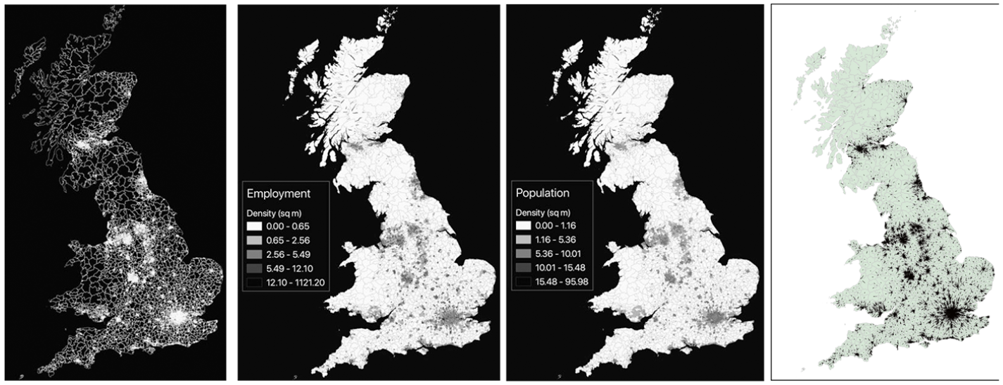
Spatial representation of the space economy: (a) MSOAs and Intermediate Zones; (b) employment density (persons/sq. mile); (c) population density (persons/sq. mile); (d) the journey to work vector field.
Figure 2 contains all the rudiments of the spatial system, the zoning system, maps of employment
There is no visualisation that can represent the flow matrices
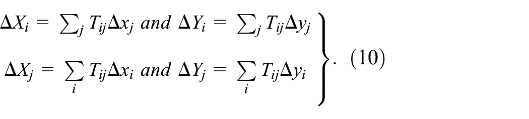
These then have to be scaled across the whole system so that they are adjusted to provide a picture of flows that are compatible with the geometry of the entire map, in other words so that these are readable and comparable.
These are but one measure of flow based on one measure of vector calculation. Others are measures of accessibility that sum over all interactions which are related to measures of potential, such as that defined originally by Stewart (1941) and first applied by Hansen (1959). We can define these too either in terms of origins or destinations from the competition terms in the basic model. From equation (1), origin accessibility for employment is defined as
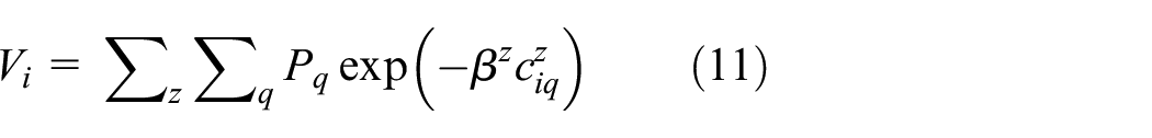
and destination accessibility for population as

We show these measures for England and Wales in Figures 3(a) and (b) for the more limited variant of the QUANT model. A comparison with employment and population densities and with the vector field in Figure 2 shows strong correlations with accessibilities, but accessibility here is a measure of ‘potential energy’ in the spirit first articulated by Stewart. However, before we demonstrate these ideas, we must introduce the kinds of impacts that are generated from the model in terms of key indicators of employment, population and change in the system of transport flows.
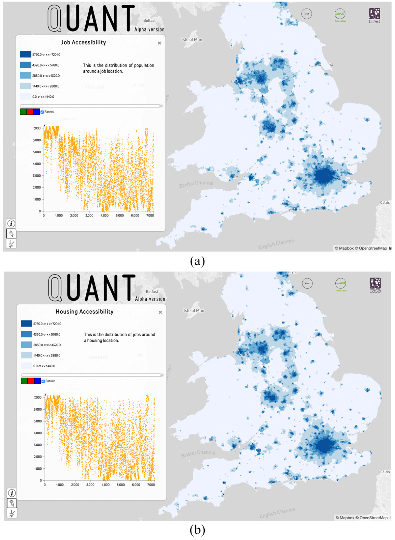
Ranked accessibility indicators: (a) employment (jobs); (b) population (housing).
Measuring and computing impacts
In the model we are able to manipulate employment, population and trips through transport costs to generate different scenarios. Changes in employment and/or population do not involve any changes in the cost matrices or their parameters, and the evaluation of scenarios based on change in the volume of activities at different locations simply involves a scaling up or down of the volume of trips dependent on these quantities. If we only alter employment say in one location, then the changes are distributed to population in proportion to the existing transport costs which produce a simple scaling up or down of the trip pattern. If many employment locations change, then the ultimate pattern of population is scaled with respect to the linear scaling associated with each employment origin. To clarify this, let us write the model in separable probability form as

where
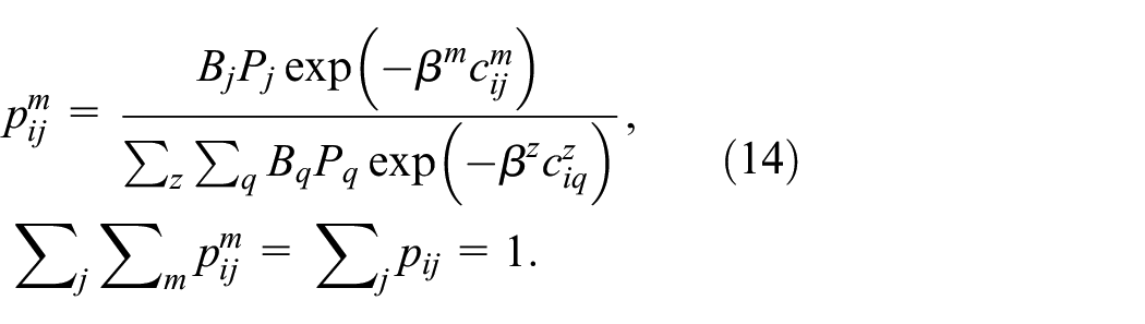
Changes in employment defined as
and noting that we assume that there is no constraint on population, that is, that

The change in employment can be positive and/or negative but as
Now more complex impacts emerge when travel costs are changed. Whereas when employment is changed the total activity varies but the distribution does not, when travel costs are changed in response to new infrastructure the repercussions can be complex and are less easy to anticipate prior to the model being run. Of course, in a fully-fledged scenario, employment, population constraints and different modal networks might all be changed and the resultant impacts are likely to be very hard to anticipate without running the model. To show how we might introduce new transport infrastructure, we will demonstrate the model equations for changes in one of the modes, consistent with introducing a lower cost route where we note that the probability in equation (13) is changed. As this is a more detailed elaboration of the impacts, we discuss these extensions in Appendix 2 but they are integral to the model scenarios introduced below.
Case studies: The impact of new employment and new rail lines
We will simply give a hint of what the model is able to predict here, focusing first on the impacts of a growth and decline in employment in a metropolitan area in North West England and then illustrating the impact of the new fast subway line across London called Crossrail. We have already used the model extensively to explore different rail and road infrastructure scenarios, such as the impact on urban development of High Speed 2, of the East West rail link in the CAMCOX corridor and of a fast rail line between Glasgow and Edinburgh. However, we will report these elsewhere as we do with the model’s full calibration (Milton et al., 2020). We will simply state the calibration here in terms of the values of the three modal parameters
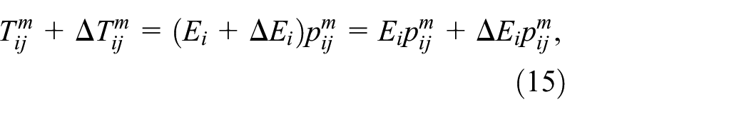
In Figure 4, we show the pattern of population in Merseyside (Liverpool and its hinterland), where we evaluate the impact of two major changes in employment – a loss of 10,000 jobs from Liverpool city centre and an inward investment of some 20,000 jobs into the Knowsley area on the eastern edge of Liverpool, the locations of which are shown in Figure 4(a). These locations are in areas where there have been substantial problems of decline in employment, although the predictions are straightforward. We show the new pattern of jobs in Figure 4(b), which is the same as the existing pattern but with those job changes shown in 4(a) determining the new pattern of working population in 4(c). These changes are generated using the model equations (13) to (16). The difference between the observed and predicted working population is shown in Figure 4(d), where it is clear how the loss and gain in jobs is distributed in terms of the working population, as predicted from equation (16). If we were to include many more changes in jobs in different zones, which would be a much more realistic scenario, then the predicted patterns would be much more complex additions and subtractions of populations, but in this simplest scenario with only two changes the predicted patterns are easy to trace. Essentially, job loss in central Liverpool leads to population loss around the central zone, while job gain in Knowsley leads to job gain around that zone – with some conjunction of these patterns due to the fact that every location is related to every other.
Job loss in central Liverpool and inward investment in East Liverpool: (a) scenario data input; (b) distribution of employment; (c) distribution of working population; (d) predicted job loss and gain in the entire region (country).
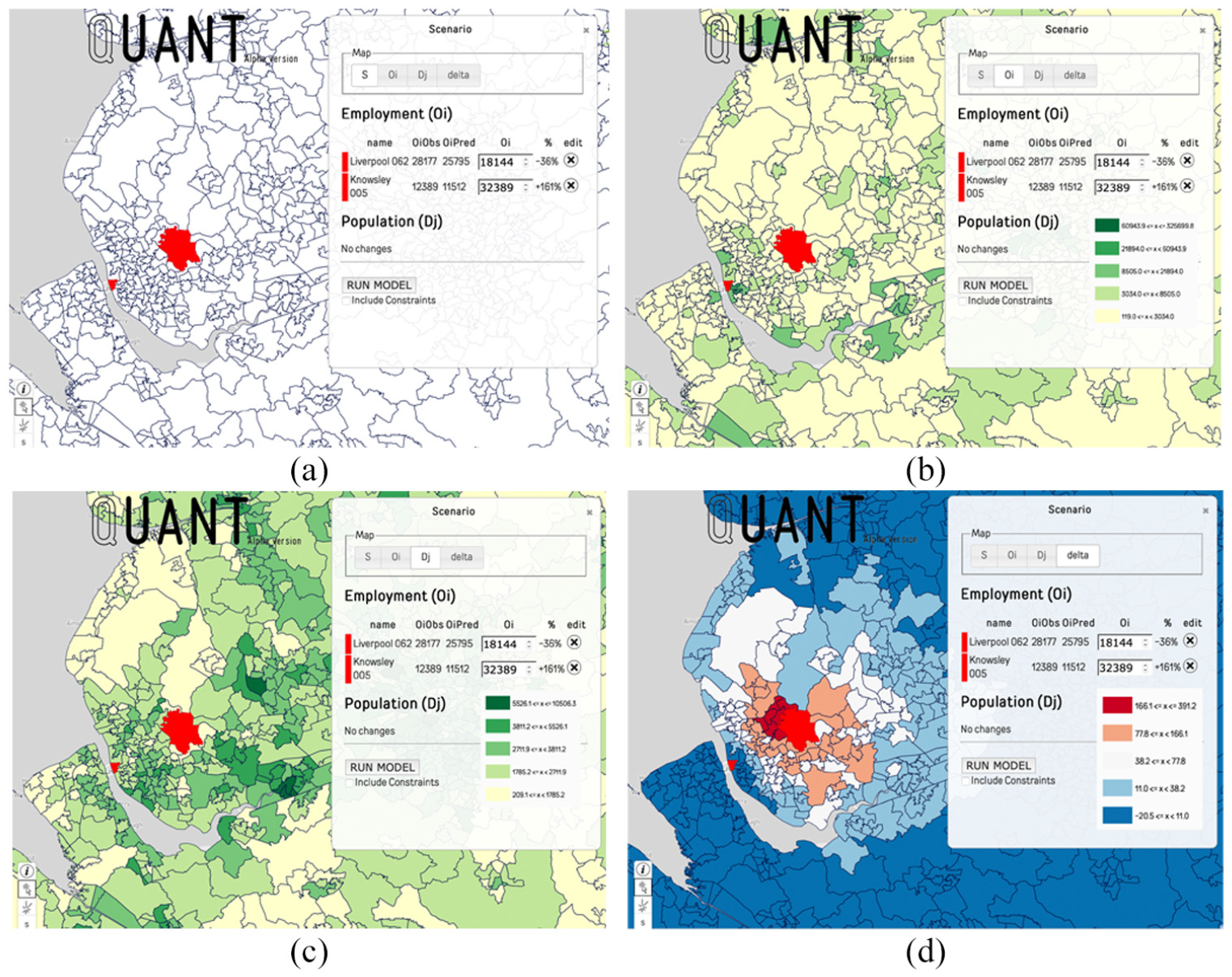
To illustrate the wider impact of interrelated changes in transportation in the model, we will briefly sketch the impact of a new high speed subway line across London. This is the Crossrail 1, a project many years in the making that links Reading in the West to Shenfield and Abbey Wood in the east of the metropolitan area, through the mainline stations north of the Thames in central London, and Heathrow airport. We show the line in Figure 5(a). The new rail line is grafted onto the existing rail network, with some additional sections constructed anew, and this is reflected in the reduced travel costs which are factored into the overall national network through running the shortest routes algorithm for rail only. The model then predicts changes in the modal split using equations (2.1) to (2.6) in Appendix 2, where there are no changes in any of the other modes so the shift in population is due to the increased attraction of the new rail line to travellers on any other mode. In short, the line attracts travellers from other modes and in Figure 5(b) we show the numbers of travellers from other modes, summing these over origins to generate the total additional population in each zone that comes from the impact of Crossrail. We can then also show the redistribution of the total population from all modes using equations (2.7) to (2.10), and these show the gains and losses in population which sum to zero in equation (2.10). We show these in Figure 5(c).
The impact of Crossrail: (a) the line as under construction; (b) shifts from all modes to rail measured by total population; (c) redistribution of the population; (d) number of improved journeys due to Crossrail.
There are many measures of impact, and in subsequent articles we will detail these and employ them as part of our scenario generator, which is yet to be constructed but is a crucial component in the use of this model for exploring urban futures. But a simple measure of impact is a count of the number of improved journeys by travel time from every station on the entire network. These are journeys that will use Crossrail, i.e. journeys that from any station to any other will improve their travel times due to the use of Crossrail, and their impact is of course very wide. In fact, all stations will produce some improvement in that the network is strongly connected and every node is linked to every other node directly or indirectly. Thus, there will be at least a connection from any station to a Crossrail station. Figure 5 provides a good visual justification for the development of models like this for an entire country.
Next steps
The framework introduced here exploits the power of modern computation in ways that enable us to handle compute-intensive models, and big data which is big because of its spatial extent, the relationships between its elements and its continued use and reuse. As the modelling framework is available to anyone at any place at any time, it can generate very large numbers of users, each spawning the application separately from one another and hence blowing up the bigness of these models by using the same data and model in parallel. Scale and size are thus compounded through many applications, hence the focus here has been to demonstrate how such problems can be tackled and made manageable for many potential users. Our model runs as a web service, and in this sense it can be nested within other systems that engage other kinds of user. A prototype is available for England and Wales at http://quant.casa.ucl.ac.uk/ and it can be run on many different devices, from a smartphone through to any kind of desktop computer, which of course have access to the internet. In fact, the model can be run from within any web-based conferencing system such as Zoom in that many participants in a Zoom session can see the model being run by one of these participants or even by all of them if they are all logged on and sharing their screens. Given the current limits on such conferencing technology, only one screen can be shared but it is only a matter of time before many will be able to share and run the same model in parallel from their own devices. The universality of computing is being continually demonstrated by such interactions and recursions.
As this is the first article to outline this new framework, there are several directions which we are exploring and which will be reported in time, four of which we will use to focus this discussion on future work. First, the full model is still under rapid development and, as we reported earlier, this will increase the time linearly with respect to the number of classes associated with any disaggregation of the employment and population variables, and nonlinearly in terms of any disaggregation of the trips by the same categories. As we add sectors, this will increase the model run time, and very soon with only a modest number of additional categories and sectors the model will take too long for the kinds of immediacy we require here. Much depends on access to fast computation and we are already experimenting with running the model on a Microsoft Azure Cloud server using the Turing Institute’s resources, thus reducing the running time by an order of magnitude. Second, we need to speed up shortest routes calculations and it is very likely that we will have to introduce approximations to enable us to handle the kind of extensive networks from which our own networks of interactions between zones are built. This relates to a third problem, and that is that this model needs to link to models built by different users at different scales, such as the LUISA family of models and its variants developed by Echenique et al. (2013) and Wan and Jin (2017). We explore this in more detail in the sister article by Milton et al. (2020).
The fourth direction is to develop a scenario generator based on the idea that the solution space of these models is massive and some means of systematically searching it is required. We can only generate hundreds of alternatives within an evolutionary design process that continually improves the search for ever-better urban futures if we have ever-faster models which enable us to proceed in this way. There have been many speculations in the past about ways this might be done (see Harris, 1967, 1971), but there are now new techniques for exploring such spaces in that if the models can be run fast enough, then many solutions can be developed to define the configuration of such spaces. The fifth area of future research and application involves improvements to the human computer interface, and this is a continuing area where the model and its usage can be made more user friendly. For many years, this has been an urgent need for the application of formal methods in planning practice, but so far the recognition and the resources necessary for developing and testing widespread applications have not been forthcoming. We estimate that the amount of resource required to enable these kinds of models to be more widely used in practice will require a tenfold increase, and most of this requires the resource to be used in educating a wide variety of researchers, planners and policy makers into the best ways of using such tools. However, to pursue all these directions, these kinds of model must be embraced by users who have enough skill and awareness to be able to use them in planning support, to generate plans and to test ‘what if?’ style predictions. This remains one of the greatest challenges in using big data and large-scale models in a way that links good theory to good practice.
Footnotes
Appendix 1
Appendix 2
Declaration of conflicting interests
The authors declared no potential conflicts of interest with respect to the research, authorship and/or publication of this article.
Funding
The authors disclosed receipt of the following financial support for the research, authorship and/or publication of this article: The Future Cities Catapult funded the early stage of this research (2016–2018) and the QUANT model is now supported by the Alan Turing Institute under QUANT2–Contract–CID–3815811. Partial support has also come from the UK Regions Digital Research Facility (UK RDRF) EP/M023583/1 through EPSRC.