Sage Journals: Discover world-class research

Abstract

Chinese

The effective, efficient and equitable policing of urban areas rests on an appreciation of the qualities and scale of, as well as the factors shaping, demand. It also requires an appreciation of the factors shaping the resources deployed in their address. To this end, this article probes the extent to which policing demand (crime, anti-social behaviour, public safety and welfare) and deployment (front-line resource) are similarly conditioned by the social and physical urban environment, and by incident complexity. The prospect of exploring policing demand, deployment and their interplay is opened through the utilisation of big data and artificial intelligence and their integration with administrative and open data sources in a generalised method of moments (GMM) multilevel model. The research finds that policing demand and deployment hold varying and time-sensitive association with features of the urban environment. Moreover, we find that the complexities embedded in policing demands serve to shape both the cumulative and marginal resources expended in their address. Beyond their substantive policy relevance, these findings serve to open new avenues for urban criminological research centred on the consideration of the interplay between policing demand and deployment.

Keywords

anti-social behaviour big data crime policing public welfare and safety

Introduction

The nature of the calls-for-service to police forces, which constitute one measure of public demand for policing, is changing. In addition to crime and anti-social behaviour (ASB), increasingly calls-for-service relate to public safety and welfare (PSW) (Boulton et al., 2016; Charman, 2018; College of Policing, 2015; Wuschke et al., 2018). Calls-for-service classified as relating to crime include all incidents that may result in a notifiable offence, whereas those classified as ASB include incidents relating to unacceptable behaviours that cause alarm or distress, and those classified as PSW include incidents relating to civil disputes, concerns for safety, domestic incidents, missing persons and suspicious circumstances (Home Office, 2011). An assessment of the calls-for-service that police forces in England and Wales responded to in 2016/2017 found that only 24% were crime related, 12% anti-social behaviour related, whilst 64% were non-crime related (inclusive of PSW) (National Audit Office (NAO), 2018). This being said, an in-depth study of calls-for-service across six police force areas found that in 90% of incidents a crime took place or held the potential to take place (Her Majesty’s Inspectorate of Constabulary (HMIC), 2012: 6). This growth and shift in demand has been attributed to the austerity agenda, which has resulted in a substantial reduction in the non-policing public services provided by the state (Crawford et al., 2019), leaving the police as a ‘service of first resort, rather than last resort’ for dealing with vulnerable people (Winsor, quoted in Her Majesty’s Inspectorate of Constabulary and Fire & Rescue Services (HMICFRS), 2018). Set against this context, there has been a limited endeavour to account for this broader palette of demand for police services (Boulton et al., 2016; Hope et al., 2001; NAO, 2018), partly attributable to the lack of reliable data (College of Policing, 2015). The requirement to advance such a project is pressing, particularly as the police in England and Wales have been subject to a significant reduction in funding (19% in real terms; NAO, 2018) over the last decade, resulting in 20,000 fewer police officers (Home Office, 2019), and reduced capacity to supply front-line resource in response to demand. Whilst the modelling of demand for and supply of policing services has tended to take place as separate exercises (Laufs et al., 2020), it is surely the case that the effective, efficient and equitable policing of urban areas rests on the interplay between the demand for and supply of police services, while evaluating the extent to which effectiveness, efficiency and fairness are achieved. Therefore, due attention should be paid to the complex social (demographic and economic), physical and policy factors underlying both. In this article, we consider these issues, using calls to the police for assistance as our measure of demand and subsequent police resource deployment as our measure of supply.

There has been longstanding recognition that crime (at least) concentrates in particular areas of cities (Sherman et al., 1989; Weisburd et al., 2012) and at certain moments in time (Brunsdon et al., 2007; Newton, 2015). Whilst the criminological endeavour to explain the where, when, why and whom of crime has often been fragmented (Bannister et al., 2019), each strand has typically considered the social (economic and demographic profile) and physical characteristics of the city, as well as the volume and recurrent mobility of its citizenry, to be important explanatory variables. These insights provoke the following research questions: Do recorded policing demands (as these relate to crime, anti-social behaviour and public safety and welfare situations) exhibit comparable spatial and temporal clustering? If they do, how are such policing demands being conditioned by the urban environment?

Previously, police forces in England and Wales used an Activity-Based Costing approach to account for the resources they committed to particular activities, but this ceased in 2008 due to the administrative and methodological (data) challenges it posed (Wain and Ariel, 2014). Here, we renew attention to this task. In this context, it is obviously the case that police deployments to a call-for-service can result in widely varying resource consequences and simple counts of calls-for-service, therefore, will fail to capture the resources committed in their address. To attend to this issue, the research utilises a big data resource, namely Airwave/GPS data, to analyse deployment patterns including resource effects. Moreover, and through the text mining of a further big data resource, namely the unstructured narratives that are attached to each call-for-service, we are able to begin to assess the complexities embedded in individual calls-for service and the marginal resource they consume. Cumulatively, these data enable us to address a further research question: To what extent is policing deployment, inclusive of both cumulative and marginal front-line policing resource, conditioned by the social and physical urban environment, and by individual incident complexity?

Policing demand and deployment, and big data

Explaining crime in the city

The spatial concentration of crime and anti-social behaviour (well reflected in policing demand as measured by calls-for-service), most prominent at small spatial units of analysis (Sherman et al., 1989), is suggestive of a ‘…“tight coupling” of crime with the places where crime occurs’ (Weisburd et al., 2012: 10). Criminological literatures, interpreted through a specific and explicit urban filter, collectively imply that crime and anti-social behaviour (and plausibly activities relating to public safety and welfare, noting that in the vast majority of such incidents a crime holds the potential to take place (HMIC, 2012: 6)), are a complex spatial and temporal consequence of the social and physical characteristics of the urban environment. Specifically, of the interplay between neighbourhood characteristics, land use features and recurrent population flows (Bannister and O’Sullivan, forthcoming). Neighbourhood characteristics can serve to influence the capacity of a community to inhibit crime and offending through the exercise of informal social control (Sampson, 2006; Shaw and McKay, 1942). A multitude of factors have been evidenced to influence informal social control at the neighbourhood level, in particular the presence/severity of poverty or deprivation (Higgins et al., 2010; Hipp, 2007), housing tenure (Livingston et al., 2014), demographic structure (Morenoff et al., 2001), family disruption (Sampson and Groves, 1989), residential stability (Sampson et al., 1997) and the level of ethnic diversity (Sampson et al., 1997). More deprived and segregated neighbourhoods tend to have worse crime outcomes due to a combination of negative socialisation, limited social networks, stigmatisation and limited access to effective institutions and resources (Livingston et al., 2014), cumulatively serving to inhibit informal social control and (potentially) attract offenders.

Land use features can influence the type(s) and volume of crime and anti-social behaviour that take place in an area (Brantingham and Brantingham, 1993; Taylor and Gottfredson, 1986; Wo, 2019), through acting as either crime generators (drawing in population groups) or crime attractors (drawing in offenders) or both (Brantingham and Brantingham, 1995). For example, areas comprised of risky facilities (Bowers, 2014), such as alcohol outlets, serve as magnetic places (Boivin and D’Elia, 2017), attracting pools of potential offenders and victims.

Recurrent population flows, the space–time geography (Hägerstraand, 1970; Miller, 2005) of the citizenry, also serve to shape the scale and mix of motivated offenders, victims and guardians (Cohen and Felson, 1979) drawn to a given setting in a given period of time. Such flows are framed by physical limitations to movement (capability constraints), the requirement to undertake mandatory societal roles (e.g. work, education) in specific locations and at particular times (coupling constraints) and the accessibility of specific locations or facilities (authority constraints). The quantification and qualification of recurrent population flows pose a significant challenge, however. Although multiple approaches have been explored, including the use of mobile phone and travel survey data (Haleem et al., 2020; Lee et al., 2020), such measures have proved unable to fully capture the dynamism of urban populations or their varied propensity to perform the roles of motivated offender, target (victim) or guardian (Hipp, 2016). Nevertheless, it remains important to recognise that both the scale and characteristics of the population present in a given setting at a given time can influence the volume and type of crime and anti-social behaviour that take place. In this regard, it is plausible that both neighbourhood and land-use characteristics, when assessed with reference to capability, coupling and authority constraints, are indicative of population flows if not their exact volume.

Explaining supply in the face of demand: Determinants of police deployment and resourcing

To date, scant scholarly attention has been afforded to the assessment of the patterning and drivers of the supply of reactive policing, that is, the deployment of front-line resources. The current UK Government police funding allocation formula is founded on a cumulative assessment of the factors driving demand at police-force level and assumptions about consequent responses. Yet, and in part as a consequence of Activity-Based Costing ceasing in 2008, the funding formula has been determined as outdated and unfit for purpose (House of Commons Home Affairs Committee, 2015). In its stead, a simplified funding model has been proposed, based on an assessment of the factors that correlate strongly with ‘long term patterns of crime and overall policing demand’ (House of Commons Home Affairs Committee, 2015: 6). Five key factors are incorporated in this model, which have resonance with the neighbourhood or social characteristics (households with no adults employed; ‘hard-pressed’ population;¹ council tax band D equivalent properties),² landuse or physical characteristics (licensed bar density) and recurrent population flows (population size) of the city (Home Office, 2015). The revised formula has yet to be implemented, as the model attracted substantial criticism from police forces during a consultation period (House of Commons Home Affairs Committee, 2017) for its alleged failure to fully encompass the factors shaping demand and the situational factors or complexities that impact on the resources consumed in addressing that demand. These are issues that remain to be investigated.

If the supply of reactive policing, that is, the deployment of front-line resources, matches or is proportionate to the patterns of overall demand, then we should expect it to be similarly tempered by the same urban characteristics. Constrained by limited resources, police forces determine whether and how quickly to deploy to a call-for-service based on an initial assessment of its severity, that is, the threat, harm and risk that the incident poses to the public or to property (NPCC Performance Management Coordination Committee, 2017). The higher the assessment of incident severity, which may vary according to its nature, the more likely and quicker the deployment response. In contrast, those calls-for-service assessed to be of low severity tend to be resolved through a telephone call or via a referral to another organisation and to be actioned over a longer time period. Calls-for-service may vary not only in their severity, but also in their complexity (College of Policing, 2015). Situational factors relating to the present or previous circumstances or vulnerabilities of the individuals involved, as well as to the nature of the incident itself, impact upon the time required to resolve it. Typically, the more complex an incident, the greater resource required in its address (College of Policing, 2020).

Aside from neighbourhood social characteristics, which can be understood as area-based measures of vulnerability, two specifically personal attributes in the form of the mental health status and/or recent alcohol consumption activity of incident participants are known to contribute to incident complexity. Moreover, individuals with mental health disorders are more likely to have contact with the police, as either a victim or an offender (McManus et al., 2016). For example, it has been estimated that between 2% and 20% of suspects passing through police stations have a mental health disorder (Bradley, 2009). Likewise, the Crime Survey of England and Wales (CSEW) reports that over half of violent incidents involving adults were perceived to be alcohol related (Flatley, 2015). Similarly, a study in the North East of England found that 93% of officers perceived that alcohol played a large contributory role in domestic abuse, whilst 60% of officers stated that alcohol-related crime and disorder took up at least half of their time (Balance – The North East Alcohol Office, 2013).

Summarising the above, both theoretical considerations and prior empirical analysis lead us to expect that patterns of police deployment and resource commitment to calls-for-service are conditioned by the same factors underpinning the demand for these services, but these patterns will also be affected by the personal characteristics and circumstances of participants within incidents further mediated by the total resources made available to the police for the purpose of dispensing their responsibilities.

The role of big data in the measurement of demand for and supply of police services

Police forces are ‘data-rich’ organisations, capturing real-time information that can be exploited via big data methods to deliver and/or confirm efficient, effective and equitable service delivery in an age of austerity, broadening demands and a heightened call for public accountability (Murphy et al., 2017). In these terms, routinely captured data on operational IT systems present new opportunities to quantify and qualify reactive policing deployment. Two particular data sources are noteworthy. Firstly, and in line with advances in mobile technologies, police forces now routinely use Geographical Positioning Satellites (GPS) (Walker and Archbold, 2018). Police officers now leave a passive and precise spatial and temporal footprint through digital radios and patrol vehicles, providing real-time volunteered geographic information (Goodchild, 2007). GPS data have begun to be used to understand the consequences of police deployment, such as the relationship between the ‘dosage’ of police patrols and the level of crime and disorder (Ariel et al., 2016). Thus, GPS data allow quantification (scale and duration) of the policing resources deployed to incidents, enabling an assessment of the complexities embodied in incidents as measured by the front-line resources they command. Secondly, police forces record the narrative of an incident in a text log. Assessment of these data, via the utilisation of text-mining algorithms, has begun to show promise in providing detail of the qualities of incidents and the characteristics of those people involved (Haleem et al., 2019). Below, we combine these data to partially rectify the limitations of previous research in the field.

Data and analytical strategy

The research study area is that of Greater Manchester (GM), a large metropolitan region located in the North West of England. GM consists of 10 local authorities with a population of 2.5 million (Office for National Statistics (ONS), 2019). Manchester city centre is the dominant employment, retail and leisure centre in the region, though there are multiple other town/city centres. This study utilises the Lower Layer Super Output Area (LSOA) geography, which is part of the UK Census geography and for which a standard set of socio-demographic and land use data sets are regularly published. There are 1673 LSOAs across GM, with each containing approximately 1600 persons (ONS, 2019). LSOAs differ in geographical size, varying between 0.05 and 25.68 km² with a median of 0.39 km², depending on residential population density.

Dependent variables

The research utilises data sets provided by Greater Manchester Police (October 2016 – September 2017), specifically calls-for-service and Airwave/GPS data, to create measures of policing demand and deployment. A call-for-service is created by the public (a 999 or 111 call), another agency (e.g. the ambulance service) or the police, and is classified in line with national standards for incident recording (Home Office, 2011). Each incident has a unique date, time, location (geocoded) stamp and response grade. The response grade serves to denote the policing judgement of the severity of the incident, that is, the decision whether to deploy front-line resource to that incident or to seek an alternative means of resolution such as a telephone call. The research only uses incidents classified as crime, anti-social behaviour (ASB) and public safety and welfare (PSW). GPS data collected by means of digital Airwave radios capture police officer resources deployed to incidents, undertaking routine patrols or investigative duties, as well as the duration of these activities. These data also possess fine-grained spatial (geocoded) and temporal (timestamp to seconds) characteristics.

Using the above data, four continuous dependent variables were generated: D1, a count of all calls-for-service or incidents classified as being crime, ASB or PSW; D2, a count of all incidents deployed to following an assessment of their severity (threat, harm and risk), but excluding those incidents to which deployment time was less than one minute; D3, a count of the cumulative time of officer deployment to an incident, recognising that an incident may have multiple officers deployed to it (this task is made possible by the GPS data, which record a unique incident reference number and the officers deployed to it); and D4, the marginal or variance around the mean resource deployed to an incident.

Independent variables

The research uses data sourced from the 2011 census (ONS, 2019), as well as Ordnance Survey Points of Interest® (POI) data, to generate a range of social and physical variables reflective of the urban environment. Census data are used to generate measures of family structure, age structure, ethnicity, income deprivation, population turnover, tenure mix, housing type and population (residential and workplace) for each LSOA. CACI ‘ACORN’ (A Classification of Residential Neighbourhoods) data are used to generate a measure of hard-pressed neighbourhoods, in line with the proposed funding formula, for each LSOA. POI data are used to determine the land use (work, education, shopping, recreation and leisure) of non-residential LSOAs, in line with the approach adopted by Lee et al. (2020). Utilising Shannon’s dissimilarity index (Shannon, 1948), these data are combined with a count of residential properties to calculate a mixed land-use variable, a measure of the abundance or evenness of land-use types across space (Dong et al., 2018). Town centre loci (capturing 52 LSOAs) were identified using the Ministry of Housing Communities and Local Government (2004) data set and used to calculate the distance between each residential LSOA centroid and a city/town centre in the GM area (monocentric and polycentric variables). Finally, police incident logs were used to assess the presence of a mental health and/or an alcohol consumption qualifier in any given incident.

Analytical strategy

The analytical strategy comprised three phases, the first being data processing. The Airwave/GPS data were transformed to enable calculation of police personnel deployment. The sheer scale of the GPS data (270 GB) made conventional processing methods impossible. Therefore, we used Hadoop clusters to maintain, manage and process the data (Yuan et al., 2015). Hadoop clusters enable big data to be managed via a distributed file system, which facilitates processing across clusters of computers using simple data models, significantly accelerating data processing time. Thereafter, the data were processed to create dependent variables, as defined in the preceding section, at LSOA level across GM. The dependent variables were then partitioned into specific time bins, reflecting the daily patterns of policing demand, according to the time at which the incident was first recorded, namely: T1, night-time (00.00–05.59); T2, morning (06.00–11.59); T3, afternoon (12.00–17.59); and T4, evening (18.00–23.59).

Unstructured text incident narratives were processed using an automated deep-learning-based text-mining approach to identify the presence or not of alcohol and/or a mental health qualifier at an incident; these are coded as a binary representing their presence (1) or absence (0). Specifically, we developed a Convolutional Neural Network (CNN)-based deep learning methodology capable of flagging incident text narratives with an affirmative reference to mental ill health and/or alcohol, whilst ignoring a negative reference to the same (Haleem et al., 2019). The CNN was designed with reference to a training data set in which incidents were classified manually by an experienced police officer and civilian researchers, with the final classification based on mutual consensus. The second phase of the analytical strategy involved an assessment of the spatial association between demand types, and across demand (D1) and deployment (D2–D4) measures in the periods T1–T4. This entailed both descriptive and correlation analysis as well as an evaluation of the spatial autocorrelation of demand (incident counts) and deployment, for which we used a Global Moran’s I test (Moran, 1950).

The third phase of the analytical strategy centred on the assessment of whether policing demand (D1) and deployment (D2–D4) are similarly conditioned by the social and physical urban environment, and by incident complexity. To this end, a two-level random intercept model accounting for the nested random effects of the spatial unit of analysis is deployed. It encompasses both time-variant (level 1) incident complexity qualifiers and time-invariant (level 2) social and physical urban environment indicators (level 2). As a first step, a multilevel model without a random intercept was deployed in order to identify significant independent variables and to test for the multicollinearity of time-invariant indicators. This reference model specification can be expressed as follows:

\log (Y_{it}) = β_{0} + β_{1 t} Q_{it} + ε_{it}

Where, $Y_{it}$ represents the dependent variables (D1, D2, D3 or D4) for each area $i$ in a particular time period (T1–T4) over the course of the day. $Q$ represents the fixed effects of the time-variant incident complexity qualifiers (alcohol and mental ill health). $ε$ is the residual error term. The random intercept $β_{0}$ represents a latent variable, the base level of the variance in policing demand across spatial units. This model is then expanded as follows:

\begin{matrix} β_{0} = γ_{00} + γ_{01} X_{1 i} + γ_{02} X_{2 i} + \dots + γ_{0 k} X_{ki} \\ + μ_{0 i} \end{matrix}

Where, $k$ is the number of time-invariant indicators $X$ by each regression coefficient $γ_{01}$ to $γ_{0 k}$ with an overall regression intercept $γ_{00}$ . The unexplained random effect $μ_{0}$ refers to the random error component, which allows for different levels of intercept with the spatial unit. These two components can then be incorporated from the random intercept model as a fixed component of the multilevel model.

The analysis addresses the issue of potential endogeneity in the social and physical urban environment indicators by assessing the extent to which explanatory variables are correlated with the error term in the multilevel model. By adopting this approach, the % income deprived population is determined, via the Hausman test, to serve as an internal instrumental variable (IV) regression estimator for level 2 regressors. Here, we follow the approach of Kim and Frees (2007) who propose adoption of a Generalised Method of Moments (GMM) estimation in multilevel modelling as an extension of instrumental variable estimators. This can be formally specified as:

\log (Y_{it}) = Z_{it} β_{0} + β_{1 t} Q_{it} + ε_{it}

Where, $Z$ denotes the instrumental variable estimators for area $i$ at a given time $t$ , in terms of the percentage of income-deprived population. By employing a GMM estimation to address endogeneity, both the between and within variations of the exogenous variables are assessed, but only the within variation of the variables is assumed to be endogenous (Kim and Frees, 2007). In other words, this approach acts to set the one or multiple regressors assumed as endogenous and to return updated parameters from random effects thereafter. This research used REndo (Gui et al., 2020) in R software to fit the model and demonstrate the bias in the random effects estimator.

Results

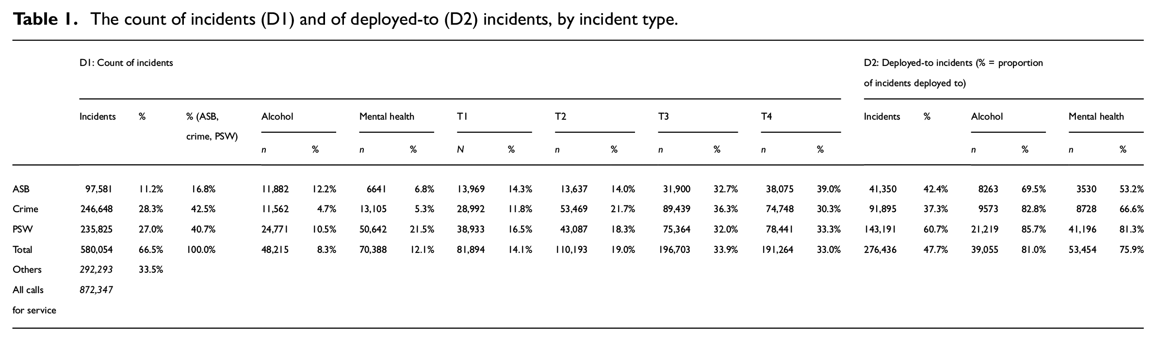
During the period October 2016 to September 2017, GMP received 872,347 calls-for-service, of which 580,054 (66.5%) were classified as ASB (n = 97,581; 11.2%), crime (n = 246,648; 28.3%) or PSW (235,825; 27.0 %). Table 1 presents the overall count of incidents (D1), and both the number and proportion of these that policing resources were deployed to (D2). In overview, less than half of all incidents (n = 276,436; 47.7%) were determined as being of sufficient severity to merit front-line officer deployment to them (i.e. they held a corresponding GPS deployment record). Of these, the text-mining approach identified that 14.1% held an alcohol marker and 19.3% a mental ill health marker. The volume of (ASB, crime and PSW) incidents varied by time of day, with the largest proportion occurring during the afternoon (T3 = 33.9%) and evening (T4 = 33%). On closer inspection, examining the hourly distribution of incidents, crime and PSW rise sharply at 07:00 and then steadily increase until 16:00. Thereafter, the level of PSW plateaus until 00:00, prior to falling sharply, whereas the level of crime falls slowly prior to dropping off from 19:00. ASB steadily rises until 18:00, and plateaus until 20:00 before falling away. For modelling purposes (D2–D4), we utilise 276,436 (47.7%) incidents with a cumulative deployment time of greater than one minute, which exhibit a mean deployment time of 163 minutes and a median deployment time of 83 minutes.

Table 1.

The count of incidents (D1) and of deployed-to (D2) incidents, by incident type.

	D1: Count of incidents															D2: Deployed-to incidents (% = proportion of incidents deployed to)
	Incidents	%	% (ASB, crime, PSW)	Alcohol		Mental health		T1		T2		T3		T4		Incidents	%	Alcohol		Mental health
	Incidents	%	% (ASB, crime, PSW)	n	%	n	%	N	%	n	%	n	%	n	%	Incidents	%	n	%	n	%
ASB	97,581	11.2%	16.8%	11,882	12.2%	6641	6.8%	13,969	14.3%	13,637	14.0%	31,900	32.7%	38,075	39.0%	41,350	42.4%	8263	69.5%	3530	53.2%
Crime	246,648	28.3%	42.5%	11,562	4.7%	13,105	5.3%	28,992	11.8%	53,469	21.7%	89,439	36.3%	74,748	30.3%	91,895	37.3%	9573	82.8%	8728	66.6%
PSW	235,825	27.0%	40.7%	24,771	10.5%	50,642	21.5%	38,933	16.5%	43,087	18.3%	75,364	32.0%	78,441	33.3%	143,191	60.7%	21,219	85.7%	41,196	81.3%
Total	580,054	66.5%	100.0%	48,215	8.3%	70,388	12.1%	81,894	14.1%	110,193	19.0%	196,703	33.9%	191,264	33.0%	276,436	47.7%	39,055	81.0%	53,454	75.9%
Others	292,293	33.5%
All calls for service	872,347

The spatial clustering of demand types, across demand and deployment measures, in different time periods for ASB, crime and PSW calls-for-service hold a strong spatial correlation as we progress from an incident count (D1: crime and ASB, rho = 0.876; crime and PSW, rho = 0.883; and ASB and PSW, rho = 0.842) via deployed-to incidents (D2: crime and ASB, rho = 0.869; crime and PSW, rho = 0.904; and ASB and PSW, rho = 0.847) to cumulative deployment time (D3: crime and ASB, rho = 0.786; crime and PSW, rho = 0.822; and ASB and PSW, rho = 0.784). The spatial correlation between the mean deployment time to ASB, crime and PSW incidents shows little relation (D4: crime and ASB, rho = 0.188; crime and PSW, rho = 0.183; and ASB and PSW, rho = 0.127). The temporal (hourly) correlations between demand types and across the measures of demand and deployment (D1–4) exhibit significant variation across the day. For example, examining count (D1) data, the correlation between crime and PSW rises from 06:00 (rho = 0.219) and peaks at 18:00 (rho = 0.678) prior to falling through the night to 06:00. The correlations between ASB and crime, and ASB and PSW, though lower, follow a similar patterning. Once again, D4 exhibits lower correlations and no distinct diurnal patterning. Further, there is evidence of positive, though moderate, spatial autocorrelation of demand (crime, ASB and PSW) as assessed via a global Moran’s I test of incident counts (D1, Z = 0.293), deployed-to incidents (D2, Z = 0.255), cumulative resources deployed to incidents (D3, Z = 0.282) and the mean deployment time to incidents (D4, Z = 0.139). Town and city centres comprise the dominant focal points of both demand (D1) and deployment (D2, D3), which is suggestive of their similar framing by the social and physical characteristics of the city. In contrast, town and city centres hold limited expression in the patterning of mean deployment time (D4).

Policing demand and deployment, and the city

Turning now to the regression analysis. Table 2 presents our evidence of how various features of the social and physical urban environment are associated with demand and deployment (D1–D4) in each time period (T1–T4). It displays, for each model and time period, the coefficient estimates and significance of each of the covariates. It is evident that the measures of demand (D1) and deployment (D2, D3) hold strong and significant association with factors representative of the social and physical characteristics of the city, but that these associations vary across different periods of the day (T1–T4).

Table 2.

Coefficients for the four multilevel GMM model estimation results.

Variables	Regressors	D1: Count of incidents				D2: Deployed-to incidents				D3: Cumulative time deployed-to incidents				D4: Mean time for each incident
		T1	T2	T3	T4	T1	T2	T3	T4	T1	T2	T3	T4	T1	T2	T3	T4
		Coeff (SD)	Coeff (SD)	Coeff (SD)	Coeff (SD)	Coeff (SD)	Coeff (SD)	Coeff (SD)	Coeff (SD)	Coeff (SD)	Coeff (SD)	Coeff (SD)	Coeff (SD)	Coeff (SD)	Coeff (SD)	Coeff (SD)	Coeff (SD)
Intercept		1.528*** (0.368)	1.522*** (0.263)	−1.129 (1.653)	1.273*** (0.482)	0.913* (0.48)	1.904*** (0.35)	1.927*** (0.542)	2.767*** (0.857)	3.887*** (0.739)	3.973*** (0.575)	4.596*** (0.778)	4.312*** (0.943)	2.431*** (0.591)	1.363** (0.543)	0.207 (2.242)	1.994*** (0.585)
Incident qualifiers	Alcohol	−1.663*** (0.019)	−2.307*** (0.018)	−3.295*** (0.018)	−2.451*** (0.017)	−1.212*** (0.02)	−2.163*** (0.021)	−2.464*** (0.02)	−1.793*** (0.018)	−1.457*** (0.033)	−2.381*** (0.037)	−2.633*** (0.032)	−1.911*** (0.028)	0.029 (0.039)	0.208*** (0.046)	0.216*** (0.04)	0.382*** (0.031)
	Mental health	−1.993*** (0.019)	−3.066*** (0.019)	−2.169*** (0.017)	−2.13*** (0.017)	−1.584*** (0.02)	−1.504*** (0.019)	−1.428*** (0.018)	−1.536*** (0.018)	−1.724*** (0.034)	−1.509*** (0.033)	−1.309*** (0.029)	−1.459*** (0.028)	−0.039 (0.04)	0.572*** (0.042)	0.754*** (0.038)	0.565*** (0.031)
	Both	−2.709*** (0.022)	−3.653*** (0.023)	−3.846*** (0.02)	−3.43*** (0.019)	−2.174*** (0.022)	−2.663*** (0.025)	−2.874*** (0.022)	−2.649*** (0.02)	−2.361*** (0.038)	−2.829*** (0.044)	−2.885*** (0.035)	−2.65*** (0.031)	0.051 (0.044)	0.413*** (0.055)	0.534*** (0.045)	0.534*** (0.034)
Geographiccovariates	%Aged over 65	−2.035*** (0.369)	−0.471*** (0.081)	−0.353*** (0.092)	−2.427*** (0.27)	−1.704*** (0.339)	−0.483*** (0.126)	−0.661*** (0.129)	−0.361 (1.516)	−1.655*** (0.511)	−0.862*** (0.201)	−1.02*** (0.2)	−0.054 (2.06)	0.321 (0.579)	−0.313** (0.159)	−1.118 (1.138)	0.274 (0.456)
	%Lone parents	0.233*** (0.009)	0.183*** (0.071)	1.658*** (0.588)	0.617*** (0.041)	0.03 (0.053)	0.337*** (0.044)	0.328*** (0.038)	0.248 (0.368)	0.203** (0.086)	0.603*** (0.065)	0.591*** (0.051)	0.246 (0.527)	0.181*** (0.016)	0.179 (0.136)	0.828 (0.672)	0.134* (0.075)
	%People incomedeprived	−0.425 (0.332)	0.441 (0.357)	−0.303 (0.945)	0.892*** (0.141)	−0.993* (0.512)	1.007*** (0.387)	0.374 (0.577)	0.501 (1.098)	−0.236 (0.794)	1.522** (0.617)	0.853 (0.822)	0.402 (1.815)	1.15** (0.52)	0.48 (0.681)	−1.519 (2.743)	1.075*** (0.13)
	%Social renting	4.635*** (0.544)	2.057*** (0.438)	−0.155 (0.469)	4.332*** (0.498)	4.694*** (0.681)	1.536*** (0.433)	2.212*** (0.436)	2.311* (1.315)	6.193*** (1.023)	3.14*** (0.684)	3.896*** (0.651)	3.023* (1.634)	0.648 (0.828)	1.441* (0.842)	2.65 (1.919)	0.229 (0.734)
	%Hard-pressedpopulation	3.391*** (0.358)	2.583*** (0.377)	3.833*** (0.951)	2.728*** (0.236)	3.765*** (0.555)	1.792*** (0.448)	2.86*** (0.637)	2.431*** (0.742)	3.967*** (0.857)	2.671*** (0.72)	3.167*** (0.897)	3.864*** (1.37)	0.581 (0.562)	1.639** (0.736)	2.868 (2.374)	0.426 (0.272)
	Bar density	0.951*** (0.13)	0.521*** (0.131)	−3.849** (1.75)	0.911*** (0.115)	1.276*** (0.236)	0.4*** (0.113)	0.463*** (0.123)	0.461** (0.184)	1.464*** (0.368)	0.868*** (0.177)	0.8*** (0.188)	0.637*** (0.198)	0.041 (0.208)	0.353 (0.249)	−1.582 (1.85)	−0.106 (0.181)
	Total businesspremises (z-score)	0.2** (0.081)	0.227* (0.123)	−0.982** (0.419)	−0.252** (0.123)	0.264** (0.115)	−0.064 (0.14)	−0.135 (0.109)	−0.387 (0.236)	0.102 (0.178)	−0.111 (0.218)	−0.365** (0.153)	−0.389 (0.297)	−0.077 (0.133)	0.134 (0.228)	−0.461 (0.394)	−0.025 (0.161)
	Total educationalpremises (z-score)	0.07** (0.032)	0.132*** (0.035)	0.065** (0.033)	−0.035 (0.025)	0.048* (0.027)	0.042 (0.043)	0.042 (0.044)	−0.157*** (0.061)	0.03 (0.04)	0.096 (0.067)	−0.007 (0.063)	−0.09 (0.063)	0.077 (0.047)	0.124* (0.066)	−0.032 (0.066)	−0.067** (0.033)
	Total service premises (z-score)	−0.054 (0.036)	0.029 (0.037)	0.072** (0.032)	−0.158*** (0.026)	−0.109*** (0.042)	0.028 (0.043)	0.024 (0.045)	−0.152*** (0.03)	−0.183*** (0.065)	−0.069 (0.068)	−0.138** (0.068)	−0.21*** (0.038)	0.019 (0.058)	−0.095 (0.072)	−0.212 (0.166)	−0.133*** (0.031)
	Total recreationalpremises(z-score)	0.13*** (0.027)	0.121*** (0.028)	−0.166 (0.113)	0.005 (0.027)	0.106*** (0.023)	0.088*** (0.033)	0.071*** (0.027)	−0.082 (0.079)	0.05 (0.034)	0.073 (0.052)	0.009 (0.039)	−0.146 (0.092)	0.042 (0.041)	0.011 (0.051)	−0.132 (0.133)	−0.169*** (0.036)
	Land-use mix	−0.066 (0.309)	0.189 (0.553)	8.907*** (3.318)	2.758*** (0.468)	−0.333 (0.433)	1.182** (0.591)	1.724*** (0.343)	2.83** (1.322)	1.405** (0.67)	2.645*** (0.924)	3.918*** (0.488)	4.506** (1.796)	1.417*** (0.516)	0.562 (1.017)	4.445 (3.344)	1.19* (0.655)
	Distance to city centre (as monocentric city centre)	−0.044 (0.057)	−0.104*** (0.038)	−0.102*** (0.039)	0.076 (0.096)	0.035 (0.062)	−0.159*** (0.043)	−0.135*** (0.046)	0.196** (0.08)	0.024 (0.096)	−0.188*** (0.067)	−0.069 (0.07)	0.207* (0.107)	−0.198** (0.091)	−0.029 (0.073)	0.165 (0.207)	0.317** (0.135)
	Distance to town city centre(as polycentric city centres)	0.444* (0.26)	0.859*** (0.22)	0.718*** (0.209)	−0.074 (0.242)	0.188 (0.184)	0.448 (0.274)	0.417 (0.306)	−1.299*** (0.483)	0.527* (0.28)	1.207*** (0.424)	0.503 (0.442)	−0.533 (0.464)	1.062*** (0.398)	0.746* (0.411)	−0.119 (0.57)	−0.819** (0.382)

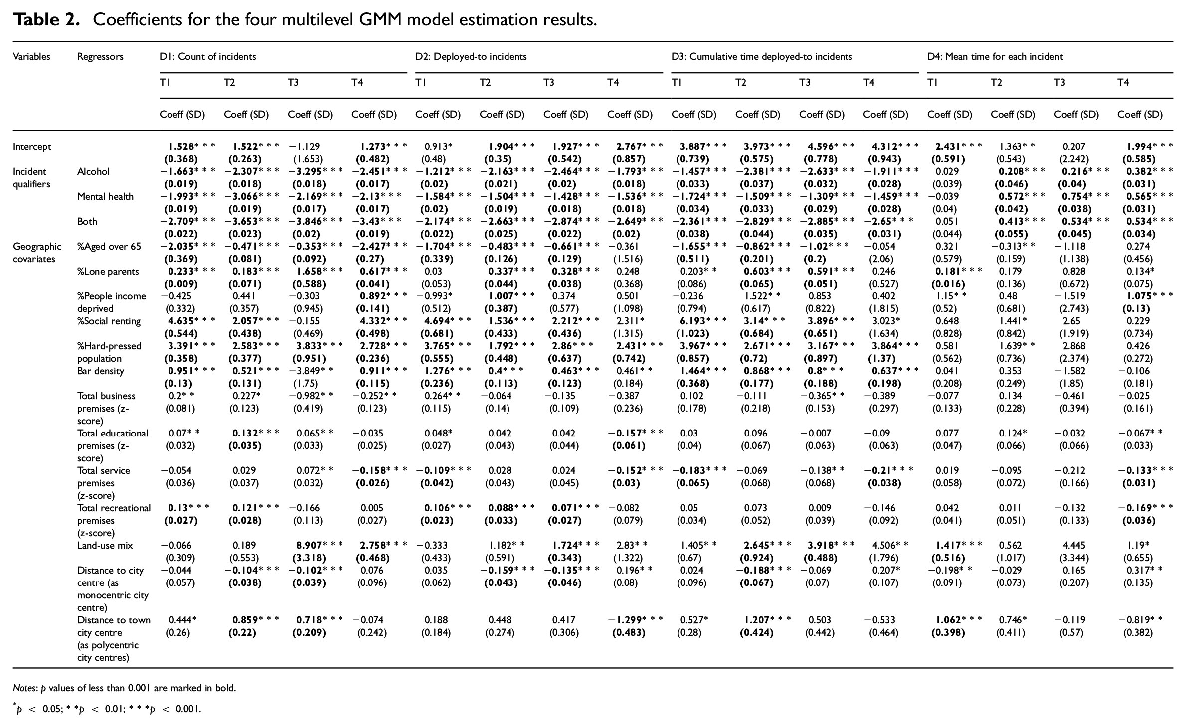
Notes: p values of less than 0.001 are marked in bold.

p < 0.05; **p < 0.01; ***p < 0.001.

Examining the count of incidents (D1), neighbourhood-based socio-economic and demographic factors (i.e. % hard-pressed population, % social renting and % lone parents as positive coefficients, and % aged over 65 as a negative coefficient), representative of the collective vulnerability of a residential population to crime, hold substantive effect. Land use-based factors, (i.e. land-use mix, bar density, business premises, recreational premises, educational premises and distance to monocentric and polycentric centres), and physical factors of the urban environment that can be understood to act as crime generators and population attractors, also hold substantive effect. Amongst both social and physical factors, there exists variation in their influence over the course of the day (T1–T4). Thus, % lone parents is particularly influential in T4, land use mix in T3 and T4 and bar density in T1 and T4. Further, some factors (i.e. bar density and business premises) exhibit both significant positive and negative effects depending on the time period under investigation.

Comparing and contrasting the influence of the social and physical features of the urban environment on the count of incidents (D1), our benchmark model, with their influence on the count of deployed-to incidents (D2), there are several noteworthy observations to make. Firstly, where similarities exist between D1, D2 and D3, they are suggestive of deployment to incidents and the cumulative time deployed to incidents being proportionate to the volume of demand generated by these factors. Secondly, and this being said, some substantive differences exist. These are particularly evident when specific time periods are taken into consideration. Thus, whereas % aged over 65 and % lone parents are significant neighbourhood-based socio-economic and demographic factors in D1 T4 (18:00 to 23.59), they are no longer significant in D2 T4. Similarly, features of the physical urban environment lose significance in D2, such as business premises (in T3 and T4), educational premises (in T2 and T3) and service premises (in T3). In other words, though influencing the volume of demand, these variables appear to hold limited influence on deployment in these time periods. Finally, distance to town and city centres (i.e. polycentric centres) in T1–T3 loses significance for D2, whereas it becomes significant and negative in T4. This finding is suggestive of deployment being focused in and around town and city centres, and the night-time economy, in T4.

Progressing to model D3, the count of cumulative time deployed to incidents, it is striking that the coefficient estimates relating to neighbourhoods with a higher percentage of hard-pressed populations and social renting rise markedly in comparison with D2. This is indicative of a greater proportion of front-line resources being required to meet deployed-to incidents in these areas, of the vulnerability of these populations and/or of the complexities of the incidents themselves. Again, there are marked differences across the course of the day. It is noteworthy, for example, that neighbourhoods with a higher percentage of social renting hold a greater influence on both deployment to incidents and cumulative time deployed to incidents during the afternoon (T3, 12:00–17:59) than they do on demand in this period. Of the physical features of the urban environment, bar density and land-use mix hold a stronger influence on cumulative time deployed to incidents than they do on deployed-to incidents per se. Once more, these findings are suggestive of the complexities embedded in these incidents, requiring greater resources to resolve. Finally, the type of premises has a lesser or insignificant effect, as does distance from city and town centres (monocentric and polycentric centres), which is now only significant in T3.

In D4, the marginal or mean variance of resources deployed to incidents, a remarkably distinct picture emerges. Here, very few of the social characteristics of the urban environment, i.e. % income deprived (T1 and T4), % hard-pressed population (T3), % lone parents (T1) and % aged over 65, retain significance, though their influence is less robust. Of the physical characteristics of the urban environment, educational, service and recreational premises have a significant negative effect, but only in T4. Land-use mix and distance from polycentric town and city centres have a significant and positive effect, but only in T1. In sharp contrast to D1–D3 (where the low count of incidents with these markers and their uneven spatial patterning lead to significant and substantial negative associations), measures of individual incident complexity, namely the presence of alcohol and mental ill health markers, hold significant and strong positive associations with the mean resource deployed to incidents in T2–T4.

Discussion

Interpreting findings

Our research findings both confirm and extend existing literatures on policing demand (HMIC, 2012) and the spatial and temporal patterning of crime (Weisburd et al., 2012). Using calls-for-service data, the results corroborate the view that the volume of non-crime (ASB and PSW) demand exceeds that of crime demand in GM. Further, and following the integration of these variables into a single demand measure, based on their strong spatial and temporal correlation, significant evidence of the clustering of demand emerged. Having established that policing demand exhibits distinct spatial and temporal patterning, we then explored the extent to which it is conditioned by the social and physical urban environment. In line with existing criminological literatures, we found clear positive (and negative) associations between a spectrum of neighbourhood social characteristics, physical land-use characteristics and the spatial and temporal patterning of policing demand.

Of these factors, neighbourhood social characteristics indicative of deprivation (% hard-pressed population, % social renting), and both family (% lone parents) and demographic (% aged over 65) structure, appear to heighten the demand for policing service and/or reduce the capacity of communities to exercise informal social control or collective efficacy (Sampson, 2006). Similarly, land-use mix, particular types of premises and city centre areas, understood as shaping the timing and volume of population flows, and thereby bringing together a pool of motivated offenders and victims (Cohen and Felson, 1979), stand out as demonstrating the greatest (positive and negative) associations with the spatial patterning of demand across different periods of the day. Whilst the literatures informing our independent variable selection and interpretation of the results were developed in an endeavour to explain the spatial and temporal patterning of crime and ASB, it is noteworthy, given that the volume of PSW calls-for-service exceeds that for crime and ASB, that they serve to substantively account for this broader measure of policing demand. In stating this, it is important to recognise that the majority of calls-for-service hold the potential to result in a crime (HMIC, 2012). In overview, the results confirm, at least to an extent, that the factors embedded in UK police funding formulas (Home Office, 2015) are reflective of the generators of policing demand.

Our research breaks new ground in assessing whether policing deployment is similarly conditioned by the social and physical urban environment. This task is vital given that the police are allocated resources based on an assessment of the factors driving demand. The analysis was enabled through the utilisation of Airwave GPS data that allow the identification of deployed-to calls-for-service (D2), and the calculation of both the cumulative (D3) and marginal (D4) resources deployed to these incidents. We find similarity and distinction between the factors associated with demand (D1; our baseline model), policing deployment (D2) and the cumulative front-line policing resource deployed to incidents (D3).

Whilst the social characteristics of the urban environment, understood as measures of neighbourhood vulnerability, retain significance (T1–T3) in the model of deployment (D2), their influence clearly weakens in comparison with the model of demand (D1). Moreover, and in T4, only the % of hard-pressed population retains significance. These findings imply that the spatial and temporal patterning of policing deployment is not closely reflected in the volume of demand associated with the social characteristics of the urban environment, particularly in the evening. However, the social characteristics of the urban environment evidence stronger association when the cumulative resource deployed to incidents (D3) is considered. In other words, those incidents deployed to in vulnerable neighbourhoods require greater front-line resource to manage, implying that they encompass greater complexity (threat, harm and/or risk).

The land-use characteristics of the urban environment, understood as time-sensitive population attractors and crime generators (Haleem et al., 2020; Lee et al., 2020), also exhibit varying influence and significance across D1–D3. It is particularly noteworthy that the influence of land-use mix and bar density appears to lessen, moving between demand (D1) and deployment (D2), but to then increase when the cumulative deployment of front-line policing resource is considered (D3). This is particularly so in T1, the early hours of the morning, a period associated with the night-time economy (Haleem et al., 2020). In a similar vein, therefore, whilst deployment holds more limited association than demand with the land-use characteristics of the urban environment, those incidents deployed to in these areas consume greater front-line deployed resource, implying that they encompass greater complexity (threat, harm and/or risk). Beyond this key finding, a number of more subtle insights can be drawn from the analysis of land-use characteristics. For example, educational premises are seen to increase demand in T1–T3, yet they are not a significant determinant of deployment or of cumulative front-line resources deployed to incidents. Here, it is plausible that, acting in a risk-averse manner, educational establishments move to report all incidents to the police but that the majority are deemed to be of insufficient severity to merit deployment or that they are resolved by other means.

In overview, this interpretation of the interplay between demand, deployment and the cumulative front-line resource deployed to incidents points to the need for deeper assessment of incident complexity. Our research begins to address this by showing how alcohol and mental ill health markers, identified through the text mining of incident narratives (logs), serve to shape the marginal or mean variance in resources deployed to incidents (D4). Both these factors are found to be significant and strong, particularly in T4. In other words, incidents involving alcohol and/or mental ill health take considerably longer to resolve by front-line policing. It is in this period that the night-time economy begins to hold sway, and that concern about vulnerable population groups is heightened (or that they become more visible).

Developing the research agenda

Given the novelty and scope of our research, proceeding from and linking the analysis of policing demand to that of deployment, our analysis is far from exhaustive and supports a call for further work in which big data is set to loom large. A number of considerations help shape the nature and form of a new research agenda. Firstly, deployment decisions no doubt reflect efforts to attain a range of institutional and personal managerial objectives on the part of police forces and officers in addition to satisfying demand, and this needs to be taken into account. Secondly, and relatedly, the decision to deploy to an incident is likely constrained by the varied capacity and capability of policing resource, across space and through time. Moreover, across (crime, ASB, PSW) and within incident categories, not all demands are equal. In these terms, deployment is always prioritised based on the assessment of the threat, harm and risk to the public (NPCC Performance Management Coordination Committee, 2017). Examining individual demand categories, and the types of incident they capture, may generate quite distinct spatial and temporal associations with features of the social and physical urban environment. Relatedly, the front-line resources required to meet these demands will reflect far more diverse measures of complexity than those captured by this research. Finally, the cumulative front-line resource deployed to incidents may only capture a fraction of the policing resource required to meet demand in that it does not take account of ‘back-office’ or investigative resources. In the round, we contend our findings serve to open and validate these new lines of enquiry, while demonstrating ways in which big data and big data methodologies might usefully be employed in the process. This agenda holds promise for the advance of effective, efficient and equitable delivery of policing across diverse urban environments, and the application of big data in the pursuit of enhanced urban well-being.

Conclusion

The demands placed upon police forces, whilst varied in nature and scale, exhibit strong spatial and temporal correlations. They cluster in particular spaces and at certain periods of the day. These patterns can be explained as arising from the complex interplay of the social and physical characteristics of the city, as well as their influence on the recurrent mobility of its citizenry. Yet, the policing of these demands, shaped by its requirement to be efficient, effective and equitable, also requires analysis (HMICFRS, 2018). As a novel investigation of policing deployment, including the front-line resources expended in responding to calls-for-service, this research made use of both big data (Airwave/GPS and unstructured text narratives) and artificial intelligence analytical techniques. Through their integration with administrative and open data sources, as well as the utilisation of more established quantitative methodologies, the research found policing deployment to be conditioned by demand but also, at least in part, by the individual complexities embedded in calls-for-service, including the nature of those incidents and the characteristics of those involved. The results highlight that a promising new approach is available for the identification and assessment of the value for money and legitimacy of policing in urban areas and that big data stands to make a significant contribution in its implementation.

Footnotes

Acknowledgements

The authors wish to express our gratitude to Greater Manchester Police for providing data sets through the Data Science/Operational Analytics project.

Declaration of conflicting interests

The author(s) declared no potential conflicts of interest with respect to the research, authorship, and/or publication of this article.

Funding

The author(s) disclosed receipt of the following financial support for the research, authorship, and/or publication of this article: This work was supported by the UK Economic and Social Research Council (ESRC) under grants (ES/P009301/1) (understanding inequalities).

ORCID iDs

Mark Ellison

Won Do Lee

Muhammad Salman Haleem

Notes

References

Ariel

Weinborn

Sherman

(2016) ‘Soft’ policing at hot spots – Do police community support officers work? A randomized controlled trial. Journal of Experimental Criminology 12: 277–317.

Balance – The North East Alcohol Office (2013) The impact of alcohol on policing in the North East. Available at: http://www.ias.org.uk/uploads/pdf/News%20stories/balance-report-march2013.pdf (accessed 15 September 2020).

Bannister

O’Sullivan

(forthcoming) Towards a planetary urban criminology. Criminological Encounters.

Bannister

O’Sullivan

Bates

(2019) Place and time in the criminology of place. Theoretical Criminology 23(3): 315–332.

Boivin

D’Elia

(2017) A network of neighborhoods: Predicting crime trips in a large Canadian city. Journal of Research in Crime and Delinquency 54(6): 824–846.

Boulton

McManus

Metcalfe

, et al. (2016) Calls for police service: Understanding the demand profile and the UK police response. The Police Journal 90(1): 70–85.

Bowers

(2014) Risky facilities: Crime radiators or crime absorbers? A comparison of internal and external levels of theft. Journal of Quantitative Criminology 30: 389–414.

Bradley

KJCB

(2009) The Bradley report: Lord Bradley’s review of people with mental health problems or learning disabilities in the criminal justice system. Report. London: Department of Health.

Brantingham

(1995) Criminality of place. European Journal on Criminal Policy and Research 3: 5–26.

10.

Brantingham

(1993) Environment, routine and situation: Toward a pattern theory of crime. Advances in Criminological Theory 5: 259–294.

11.

Brunsdon

Corcoran

Higgs

(2007) Visualising space and time in crime patterns: A comparison of methods. Computers, Environment and Urban Systems 31(1): 52–75.

12.

CACI (2010) ACORN, the smarter consumer classification: User guide. Available at: https://www.businessballs.com/freespecialresources/acorn-demographics-2010.pdf (accessed 15 September 2020).

13.

Charman

(2018) From crime fighting to public protection: The shaping of police officers’ sense of role. Perspectives on Policing: Paper 3. London: The Police Foundation.

14.

Cohen

Felson

(1979) Social change and crime rate trends: A routine activity approach. American Sociological Review 44(4): 588–608.

15.

College of Policing (2015) College of policing analysis: Estimating demand on the police service. Available at: https://www.college.police.uk/News/College-news/Documents/Demand%20Report%2023_1_15_noBleed.pdf (accessed 15 September 2020).

16.

College of Policing (2020) Supporting forces in responding to vulnerability. Available at: https://www.college.police.uk/News/Blogs/Pages/Vulnerability.aspx (accessed 15 September 2020).

17.

Crawford

Johnson

Zaranko

(2019) Chancellor ends austerity for public services – But risks breaching current fiscal rules. Press release, 4 September. London: Institute for Fiscal Studies.

18.

Department for Communities and Local Government (DCLG) (2015) Council tax levels set by local authorities in England 2015–16 (revised). Available at: https://assets.publishing.service.gov.uk/government/uploads/system/uploads/attachment_data/file/445085/150714_Revised_Council_Tax_Stats_Release_July_2015.pdf (accessed 15 September 2020).

19.

Dong

Kwan

M-P

, et al. (2018) Multi-level temporal autoregressive modelling of daily activity satisfaction using GPS-integrated activity diary data. International Journal of Geographical Information Science 32(11): 2189–2208.

20.

Flatley

(2015) Violent Crime and Sexual Offences: Alcohol-Related Violence: Findings from the 2013/14 Crime Survey for England and Wales and Police Recorded Crime Over the Same Period on Violent Crime and Sexual Offences. London: Office for National Statistics.

21.

Goodchild

(2007) Citizens as sensors: The world of volunteered geography. GeoJournal 69: 211–221.

22.

Gui

Meierer

Algesheimer

, et al. (2020) REndo: Fitting linear models with endogenous regressors using latent instrumental variables. Available at: https://github.com/mmeierer/REndo (accessed 24 August 2020).

23.

Hägerstraand

(1970) What about people in regional science? Papers in Regional Science 24(1): 7–24.

24.

Haleem

Do Lee

Ellison

, et al. (2020) The ‘exposed’ population, violent crime in public space and the night-time economy in Manchester, UK. European Journal on Criminal Policy and Research. Epub ahead of print 20 June 2020. DOI: 10.1007/s10610-020-09452-5.

25.

Haleem

Han

Harding

, et al. (2019) An automated text mining approach for classifying mental-ill health incidents from police incident logs for data-driven intelligence. In: 2019 IEEE international conference on systems, man and cybernetics (SMC), Bari, Italy, 6–9 October 2019, pp. 2279–2284.

26.

Her Majesty’s Inspectorate of Constabulary (HMIC) (2012) Taking time for crime: A study of how police officers prevent crime in the field. Available at: https://www.justiceinspectorates.gov.uk/hmicfrs/media/taking-time-for-crime.pdf (accessed 15 September 2020).

27.

Her Majesty’s Inspectorate of Constabulary and Fire & Rescue Services (HMICFRS) (2018) Policing and mental health: Picking up the pieces. Available at: https://www.justiceinspectorates.gov.uk/hmicfrs/wp-content/uploads/policing-and-mental-health-picking-up-the-pieces.pdf (accessed 15 September 2020).

28.

Higgins

Robb

Binton

(2010) Geographic patterns of crime. In: Home Office Crime in England and Wales 2009/10: Findings from the British Crime Survey and Police Recorded Crime. London: Home Office, pp. 165–194.

29.

Hipp

(2007) Income inequality, race, and place: Does the distribution of race and class within neighborhoods affect crime rates? Criminology 45(3): 665–697.

30.

Hipp

(2016) General theory of spatial crime patterns. Criminology 54(4): 653–679.

31.

Home Office (2011) The national standard for incident recording. Available at: https://assets.publishing.service.gov.uk/government/uploads/system/uploads/attachment_data/file/116658/count-nsir11.pdf (accessed 15 September 2020).

32.

Home Office (2015) Consultation on reform of police funding arrangements in England and Wales. Available at: https://assets.publishing.service.gov.uk/government/uploads/system/uploads/attachment_data/file/447083/2015_07_20_Police_funding_consultation_doc.pdf (accessed 15 September 2020).

33.

Home Office (2019) Police workforce, England and Wales, 31 March 2019. Available at: https://assets.publishing.service.gov.uk/government/uploads/system/uploads/attachment_data/file/831726/police-workforce-mar19-hosb1119.pdf (accessed 15 September 2020).

34.

Hope

Karstedt

Farrall

(2001) The Relationship Between Calls and Crimes. London: Home Office.

35.

House of Commons Home Affairs Committee (2015) Reform of the police funding formula: Fourth report of session 2015–16. Available at: https://publications.parliament.uk/pa/cm201516/cmselect/cmhaff/476/476.pdf (accessed 15 September 2020).

36.

House of Commons Home Affairs Committee (2017) Reform of the police funding formula: Government response to the committee’s fourth report of session 2015–16. Eighth special report of session 2016–17. Available at: https://publications.parliament.uk/pa/cm201617/cmselect/cmhaff/1093/1093.pdf (accessed 15 September 2020).

37.

Kim

Frees

(2007) Multilevel modeling with correlated effects. Psychometrika 72(4): 505–533.

38.

Laufs

Bowers

Birks

, et al. (2020) Understanding the concept of ‘demand’ in policing: A scoping review and resulting implications for demand management. Policing and Society. Epub ahead of print 15 July 2020. DOI: 10.1080/10439463.2020.1791862.

39.

Lee

Haleem

Ellison

, et al. (2020) The influence of intra-daily activities and settings upon weekday violent crime in public spaces in Manchester, UK. European Journal on Criminal Policy and Research. Epub ahead of print 10 July 2020. DOI: 10.1007/s10610-020-09456-1.

40.

Livingston

Galster

Kearns

, et al. (2014) Criminal neighbourhoods: Does the density of prior offenders in an area encourage others to commit crime? Environment and Planning A 46(10): 2469–2488.

41.

McManus

Bebbington

Jenkins

, et al. (2016) Mental health and wellbeing in England: Adult Psychiatric Morbidity Survey 2014. A survey carried out for NHS Digital by NatCen Social Research and the Department of Health Sciences, University of Leicester. Leeds: NHS Digital.

42.

Miller

(2005) A measurement theory for time geography. Geographical Analysis 37(1): 17–45.

43.

Ministry of Housing Communities and Local Government (2004) English town centres 2004. Towns and Cities. Available at: https://data.gov.uk/dataset/ed07b21f-0a33-49e2-9578-83ccbc6a20db/english-town-centres-2004 (accessed 15 September 2020).

44.

Moran

(1950) Notes on continuous stochastic phenomena. Biometrika 37(1–2): 17–23.

45.

Morenoff

Sampson

Raudenbush

(2001) Neighborhood inequality, collective efficacy, and the spatial dynamics of urban violence. Criminology 39(3): 517–558.

46.

Murphy

Eckersley

Ferry

(2017) Accountability and transparency: Police forces in England and Wales. Public Policy and Administration 32(3): 197–213.

47.

National Audit Office (NAO) (2018) Financial Sustainability of Police Forces in England & Wales 2018. London: HMSO. Available at: https://www.nao.org.uk/wp-content/uploads/2018/09/Financial-sustainability-of-police-forces-in-England-and-Wales-2018.pdf (accessed 15 September 2020).

48.

Newton

(2015) Crime and the NTE: Multi-classification crime (MCC) hot spots in time and space. Crime Science 4: 30.

49.

NPCC Performance Management Coordination Committee (2017) Better understanding demand – Policing the future. Available at: https://www.npcc.police.uk/2017%20FOI/CO/078%2017%20CCC%20April%202017%2024%20Better%20Understanding%20Demand%20Policing%20the%20Future.pdf (accessed 15 September 2020).

50.

Office for National Statistics (ONS) (2019) Population Estimates for UK, England and Wales, Scotland and Northern Ireland. Available at: https://www.ons.gov.uk/peoplepopulationandcommunity/populationandmigration/populationestimates/bulletins/annualmidyearpopulationestimates/mid2019estimates (accessed 15 September 2020).

51.

Sampson

(2006) Collective efficacy theory: Lessons learned and directions for future inquiry. In: Cullen

Wright

Blevins

(eds) Taking Stock: The Status of Criminological Theory. London: Routledge, pp. 149–167.

52.

Sampson

Groves

(1989) Community structure and crime: Testing social-disorganization theory. American Journal of Sociology 94(4): 774–802.

53.

Sampson

Raudenbush

Earls

(1997) Neighborhoods and violent crime: A multilevel study of collective efficacy. Science 277: 918–924.

54.

Shannon

(1948) A mathematical theory of communication. Bell System Technical Journal 27: 379–423.

55.

Shaw

McKay

(1942) Juvenile Delinquency and Urban Areas. Chicago, IL: University of Chicago Press.

56.

Sherman

Gartin

Buerger

(1989) Hot spots of predatory crime: Routine activities and the criminology of place. Criminology 27(1): 27–56.

57.

Taylor

Gottfredson

(1986) Environmental design, crime, and prevention: An examination of community dynamics. Crime and Justice 8: 387–416.

58.

Wain

Ariel

(2014) Tracking of police patrol. Policing: A Journal of Policy and Practice 8(3): 274–283.

59.

Walker

Archbold

(2018) The New World of Police Accountability. Thousand Oaks, CA, and London: Sage Publications.

60.

Weisburd

Groff

Yang

S-M

(2012) The Criminology of Place: Street Segments and Our Understanding of the Crime Problem. Oxford: Oxford University Press.

61.

(2019) Understanding the differential effects of land uses on crime: An examination across Philadelphia neighbourhoods. The British Journal of Criminology 59(6): 1432–1454.

62.

Wuschke

Andresen

Brantingham

, et al. (2018) What do police do and where do they do it? International Journal of Police Science & Management 20(1): 19–27.

63.

Yuan

Deng

Yang

, et al. (2015) A smart work performance measurement system for police officers. IEEE Access 3: 1755–1764.

Understanding policing demand and deployment through the lens of the city and with the application of big data

Abstract

Keywords

Introduction

Policing demand and deployment, and big data

Explaining crime in the city

Explaining supply in the face of demand: Determinants of police deployment and resourcing

The role of big data in the measurement of demand for and supply of police services

Data and analytical strategy

Dependent variables

Independent variables

Analytical strategy

Results

Policing demand and deployment, and the city

Discussion

Interpreting findings

Developing the research agenda

Conclusion

Footnotes

Acknowledgements

Declaration of conflicting interests

Funding

ORCID iDs

Notes

References