Sage Journals: Discover world-class research

Abstract

What are the economic consequences of college noncompletion? Given escalating student debt, is “some college” still worth it? This article applies augmented inverse probability weighting to the National Longitudinal Survey of Youth 1997 to estimate the causal effect of college noncompletion on income and financial hardship. Although noncompletion yields higher income than never attending college, it also increases financial hardship among more-disadvantaged groups through the mechanism of student debt. However, noncompleters of most groups would have had greater income and experienced less financial hardship had they graduated. Such contradictions complicate equalization and reproduction theories of higher education because higher education appears to have both equalizing (in the case of completion) and reproductive (in the case of noncompletion) effects. I argue this ambiguity is substantively meaningful, suggesting future research should examine whether the production of ambiguity constitutes a key social function of higher education.

Keywords

debt higher education inequality some college stratification

College noncompletion is common, highly stratified, and expensive. In the United States, national college completion rates have nearly doubled since the 1970s, but the increase has been unequal: Completion rates grew most among college students in the top income quartile (to 69 percent) but remained staggeringly low (26 percent) among students in the bottom income quartile (Pell Institute 2020). Across U.S. two- and four-year institutions combined, noncompletion is almost as common as earning a postsecondary degree; as of 2019, more than 36 million Americans had started college and exited without a degree (National Student Clearinghouse 2019). College costs have also risen sharply, and college students of all income levels have increasingly turned to student loans to finance their higher education—even (sometimes, particularly) in weak or uncertain employment markets (Houle 2014).

A growing body of research examines income returns to noncompletion, finding modest returns to some postsecondary schooling (Carneiro, Heckman, and Vytlacil 2011; Doyle and Skinner 2016; Giani, Attewell, and Walling 2020; Holzer and Baum 2017; Scott-Clayton and Wen 2018; Zeidenberg, Scott, and Belfield 2015). But are potential gains enough to make the costs of college noncompletion “worth it”? Costs like educational debt may undercut other economic returns and change the calculus on higher education’s equalizing effects for individuals, especially for noncompleters. Furthermore, how are returns to noncompletion distributed? At a social level, the prevalence of noncompletion among specific groups may make noncompletion significant to stratification. Higher education may not just gate-keep opportunity; it may also create hardship and do so in uneven ways. If college noncompletion has a downward socioeconomic effect for individuals or for specific groups, then institutional and structural processes that contribute to noncompletion should be studied as possible mechanisms by which social inequality is reproduced or even worsened. Higher education is often understood to have an equalizing effect among college completers (Hout 2012), but does higher education also have an equalizing effect on socioeconomic inequality when viewed from the perspective of the nearly half of all college-goers who never finish?

This article asks whether people who exit college without a degree are worse off financially than they would have been if they had never enrolled in terms of average income in their 30s and evidence of financial duress or hardship, such as taking out payday loans or being harassed by bill collectors. It also asks whether and how these financial consequences of noncompletion vary within the population.

I first discuss what can be gained by considering the debate over higher education’s equalizing or reproductive effects through the lens of college noncompletion, and I detail hypotheses that extant scholarship offers about the financial consequences of “some college.” Using the National Longitudinal Survey of Youth 1997 (NLSY97; Bureau of Labor Statistics 2019), I estimate the average treatment effects of noncompletion on income and financial hardship by applying a two-stage regression technique that uses weights to purge treatment effect estimates of observed selection bias. I find, consistent with prior research, that noncompleters have greater income, on average, than never-attenders as a result of their participation in higher education. However, I also find evidence that for some less-advantaged groups, noncompletion leads to increased financial hardship in early adulthood compared to no college, including among groups who average higher incomes as the result of attending some college, and this hardship is mediated by educational debt. By showing that most noncompleters would have earned more money and experienced less financial hardship in their 30s if they had finished their degrees (despite taking out more debt), I also argue that debates about whether people who are unlikely to finish college should enroll ought to carefully consider not just one but both relevant counterfactuals: never attending college and college completion.

The case of noncompletion illustrates how higher education can both benefit and harm individuals’ socioeconomic chances in the medium term and does so in different ways for different groups. Because returns may change over time, it also illustrates the importance of assessing returns to education throughout the life course. I conclude by suggesting that conceptualizing the apparent ambiguities or contradictions in the consequences of college noncompletion can clarify alternative ways to think about the social function of U.S. higher education beyond familiar arguments that education either improves individuals’ life chances or reifies social hierarchies.

Equalization or Reproduction?

Much scholarship on returns to college completion affirms the positive consequences of earning a bachelor’s degree. Among other benefits, students who earn a bachelor’s are more likely to earn greater income, hold higher-status jobs, and enjoy better health—enough so that earning a college degree is still more valuable than the rising costs of college (Hout 2012). Furthermore, college completion yields the greatest benefit for students who are least likely to enroll, which complicates the counterargument that selection into college (rather than credentials, connections, or skills) produces these rewards (Brand and Xie 2010; Card 2001; but see Breen, Choi, and Holm 2015). Indeed, earning a bachelor’s degree appears to weaken, and sometimes eliminate, the association between a student’s family background and their class, occupational status, earnings, and household income in adulthood (Hout 1988; Karlson 2019; Torche 2011). However, scholars disagree about whether the benefits of degree attainment accrue most to advantaged people who are already more likely to earn a degree (termed “positive selection”; see Carneiro et al. 2011; Witteveen and Attewell 2020; Zhou 2019) or whether greater returns accrue to disadvantaged people who are less likely to earn a degree (“negative selection”; see Brand and Xie 2010; Giani et al. 2020). Negative selection corresponds with the equalization hypothesis to the extent that it reduces inequality, and positive selection corresponds with the reproduction hypothesis to the extent that it perpetuates inequality (although positive selection may not always have this effect: if advantaged groups benefit the most from college completion but disadvantaged groups still gain some returns compared to never attending college, the reproductive effect is not so straightforward).

Prior work has further shown that institutional structures, practices, and processes within higher education can also reproduce the association between social origins and destinations. Restricting college access—by limiting who applies and is admitted to which colleges under what conditions and financial aid packages—is one important mechanism by which secondary and postsecondary institutions help reproduce race and class hierarchies (for a useful summary, see Serna and Woulfe 2017). Conversely, in the case of for-profit institutions, the intensive recruitment (i.e., predatory access) of low-income students of color enriches publicly traded universities while shifting the burden of risk onto vulnerable students’ shoulders (Cottom 2017). What happens after students enroll in college is also consequential: Armstrong and Hamilton (2013) demonstrate how institutional policies, programs, and sponsored organizations shunt students toward class-reproductive networks, majors, and occupations at a large, public university, and Jack (2019) reveals how social and cultural capital differences among low-income students combine with institutional practices to produce stratifying effects despite the fact that these students won admission to an elite university. Far from reducing inequality, these analyses show how higher education can help recreate it.

In other words, compelling but conflicting evidence argues that higher education has either equalizing or reproductive effects. Because it represents a different higher-education outcome than either access or completion, the case of college noncompletion is useful to this equalization-versus-reproduction debate in several respects.

The Case of College Noncompletion

Noncompletion is often studied as a counterfactual to college completion or as a source of selection bias: If people who select out of higher education are systematically similar, effect estimates of college completion among completers will be biased. Analysts therefore have accounted theoretically and empirically for noncompletion understood as part of “selective attrition” (Karlson 2019; Torche 2011). Conceptually, though, the consequences of college completion and noncompletion are different, and the consequences of noncompletion should not be understood simply as forgone advantages of college completion.

First, having attended some higher education could benefit noncompleters relative to never-attenders in several ways. “Human capital theory” argues that students who go to college accrue meaningful benefits (in the form of skills, social networks, or cultural capital) regardless of whether they exit before graduating (Becker 1964; Grubb 2002). Or, attending some college could serve as a “signal” to employers, indicating that a job candidate is a hard worker (Card 2001; Doyle and Skinner 2016; Spence 1973), which could yield labor market returns.

However, attending some higher education could also harm noncompleters relative to never-attenders. “Credential theory” argues the benefits of higher education hinge on degree attainment: Completing college endows a graduate with a socially valuable marker, a credential, which grants them particular labor market status (Collins 1979; Hout 2012; Torche 2011). From this perspective, the benefits of college depend on earning a diploma: Spending time in college without earning a degree would represent lost work experience without resulting in a credential to boost earning potential. Additionally, college costs have nearly tripled since 1975, and college is increasingly financed through student and family loans (Mettler 2014; Pell Institute 2020). Low-income students are more likely to take out loans and to take out loans in greater amounts (Huelsman 2015), which is particularly risky given their higher chances of noncompletion and loan default (Kirp 2019). If noncompleters take on substantial loans to pay for college but do not see income returns, they could be left with limited options for repaying educational debt. Furthermore, student debt is racialized and stratifying: Black students take out more debt than white students,¹ and this debt may create precarity among upwardly mobile groups, like new members of the Black middle class (Houle and Addo 2019; Seamster and Charron-Chénier 2017). Noncompletion paired with student debt could have a downward effect on socioeconomic status. If noncompletion signals failure to employers or community members, it could be associated with stigma, or diminished social capital, as a result of having “dropped out.”

A developing body of research on noncompleters tends to support human capital and signaling theories of noncompletion, having found modest income returns to some college. Comparing noncompleters to people who never attended college, recent studies estimate income returns to some college of 6 percent to 10 percent (using the NLSY97, Doyle and Skinner [2016] estimate 9.5 percent; see also Giani et al. 2020; Holzer and Baum 2017; Scott-Clayton and Wen 2018; Zeidenberg et al. 2015). Yet Carneiro and colleagues (2011) use the NLSY79 to show that while being induced to attend college because of geographic proximity leads to an earnings increase of about 9.5 percent per year of schooling among white males, the increase due to a policy that promotes college attendance is so low as to be almost negligible, at around 1.4 percent (Carneiro et al. 2011:2755).

An important question remains: How meaningful are these returns, especially if they co-occur with student debt? If income returns to noncompletion are low and educational debt among noncompleters is high, then noncompletion could create, instead of alleviate, financial burdens and exacerbate inequality. If income returns are positive but very small, noncompletion could have a negligible effect on inequality. Or if income returns to noncompletion are high relative to student debt, then noncompletion could have an equalizing effect.

A final distinction between the effects of noncompletion versus completion is that noncompletion has at least two relevant counterfactuals: never attending college and earning a degree. Both are important considerations in the context of the equalization or reproduction debate, but they are rarely examined together in existing research, if at all. (I am unaware of any such studies; “some college” analyses usually focus on one counterfactual or the other but not both. Brand, Pfeffer, and Goldrick-Rab [2014] examine similar counterfactuals but focus on community college.)

Heterogeneous Effects

Understanding potential heterogeneity is central to assessing whether or not higher education has an equalizing effect: For equalization to occur, higher education must benefit people from disadvantaged social positions at least as much as it benefits their more advantaged peers, if not more so. Similarly, if higher education has a reproductive effect on inequality, it should most benefit the already-advantaged or have negligible effects for disadvantaged groups. Recent studies differ in their findings regarding such heterogeneity. Brand and Xie (2010) and Giani and colleagues (2020) find equalizing effects of college completion on income and of college attendance on employment, respectively; Cheng and colleagues (2021) find higher education most benefits groups at both extremes of socioeconomic advantage and disadvantage; and Zhou (2019) finds that degree attainment has a reproductive effect on intergenerational rank–rank income mobility across the income distribution. Thus, effect heterogeneity remains an important topic of debate.

Two broad approaches to estimating effect heterogeneity predominate in existing literature: stratifying by demographic subgroup (using ascribed categories like race, class, and gender) and stratifying by likelihood of treatment selection (propensity score; e.g., Brand and Xie 2010; Cheng et al. 2021; Giani et al. 2020). Each illuminates a different interpretive angle. Emphasizing demographic subgroups makes it easier to focus outreach by demographic group, and it helps analysts more directly consider the link between postsecondary attainment and the labor market, where ascribed categories are associated with advantage or disadvantage. Conversely, focusing on propensity score strata helps analysts think about individuals on the margin of various attainment outcomes and integrate information about the intersecting characteristics of individual lives at the interpretive level. Because effect heterogeneity is central to my inquiry, I engage both approaches.

Current Study

My analysis responds to three main questions: (1) Are college noncompleters better or worse off financially than they would have been if they had never enrolled in college? (2) Are noncompleters better or worse off financially than they would have been if they had completed their degrees? and (3) How, if at all, do the consequences of noncompletion vary? As explored earlier, existing literature offers conflicting hypotheses about the economic consequences of noncompletion. The hypotheses variously argue that the economic effects of higher education depend on credentialing, human capital development, labor market signaling, positive selection, negative selection, opportunity costs, or stigma. To these, I add a “financial costs” hypothesis, which expects that because of student debt, noncompleters may experience more hardship than both never-attenders and completers despite potential income returns to some college.

Data

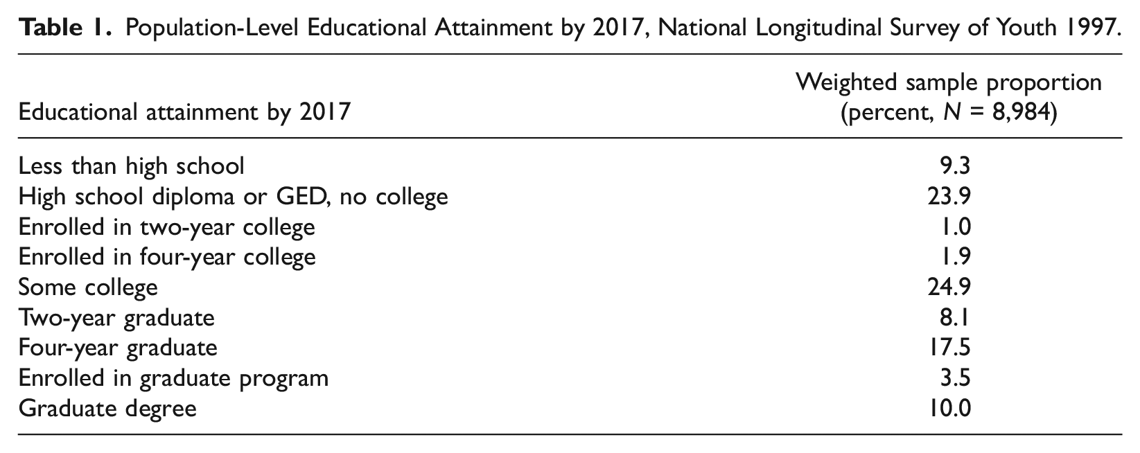
Because it surveys young adults who have lived through the recent transformations of higher education, I use the National Longitudinal Survey of Youth 1997 for this analysis. The NLSY97 is a nationally representative, ongoing study that recursively surveys 8,984 individuals from the 1980 to 1984 U.S. birth cohorts on a wide range of variables. Data through Round 18 (2017 to 2018) were available for this analysis. Nearly a quarter (24.9 percent) of respondents in the NLSY97 weighted sample started but did not complete higher education (see Table 1).

Table 1.

Population-Level Educational Attainment by 2017, National Longitudinal Survey of Youth 1997.

Educational attainment by 2017	Weighted sample proportion (percent, N = 8,984)
Less than high school	9.3
High school diploma or GED, no college	23.9
Enrolled in two-year college	1.0
Enrolled in four-year college	1.9
Some college	24.9
Two-year graduate	8.1
Four-year graduate	17.5
Enrolled in graduate program	3.5
Graduate degree	10.0

Within the NLSY97, I selected a subsample of all individuals who had earned at least a high school diploma or GED by the year they turned 29 (n = 7,482; 29 is the latest age for which sufficient income and educational debt data are available). I examine this subsample to describe the population of college noncompleters. Compared to completers, noncompleters are more likely to be Black, more likely to come from lower net-worth backgrounds, and more likely to be male (see Table 2). Broadly, this is consistent with existing literature on college attendance and persistence: College graduation rates are stratified by race and class, and more women graduate than men.

Table 2.

Descriptive Statistics by Postsecondary Completion Status, National Longitudinal Survey of Youth 1997 Unimputed Data (N = 7,482).

	Never-attender		Noncompleter		Completer
	Weighted mean or proportion	Observations	Weighted mean or proportion	Observations	Weighted mean or proportion	Observations
Lower net worth	39.1%	2,339	37.2%	2,435	31.7%	2,708
Parental attainment	1.98	2,251	2.25	2,363	2.56	2,628
Black	18.7%	2,339	18.9%	2,435	9.8%	2,708
White	70.5%	2,339	68.2%	2,435	78.9%	2,708
Female	39.1%	2,339	48.1%	2,435	56.6%	2,708
Male	60.9%	2,339	51.9%	2,435	43.3%	2,708
Urban	67.8%	2,218	76.0%	2,332	72.3%	2,633
Siblings	2.46	2,339	2.34	2,435	2.24	2,708
Father present	50.3%	2,328	55.1%	2,428	73.0%	2,703
GPA	5.54	1,471	6.06	1,759	6.98	2,115
College prep	20.2%	1,464	37.4%	1,729	65.3%	2,081
AFQT	33,237	1,760	49,214	1,979	68,008	2,328
Noncognitive	3.67	1,236	3.73	1,367	3.91	1,613
Peer college intentions	3.30	2,335	3.59	2,434	3.9	2,708
Total N	—	2,339	—	2,435	—	2,708

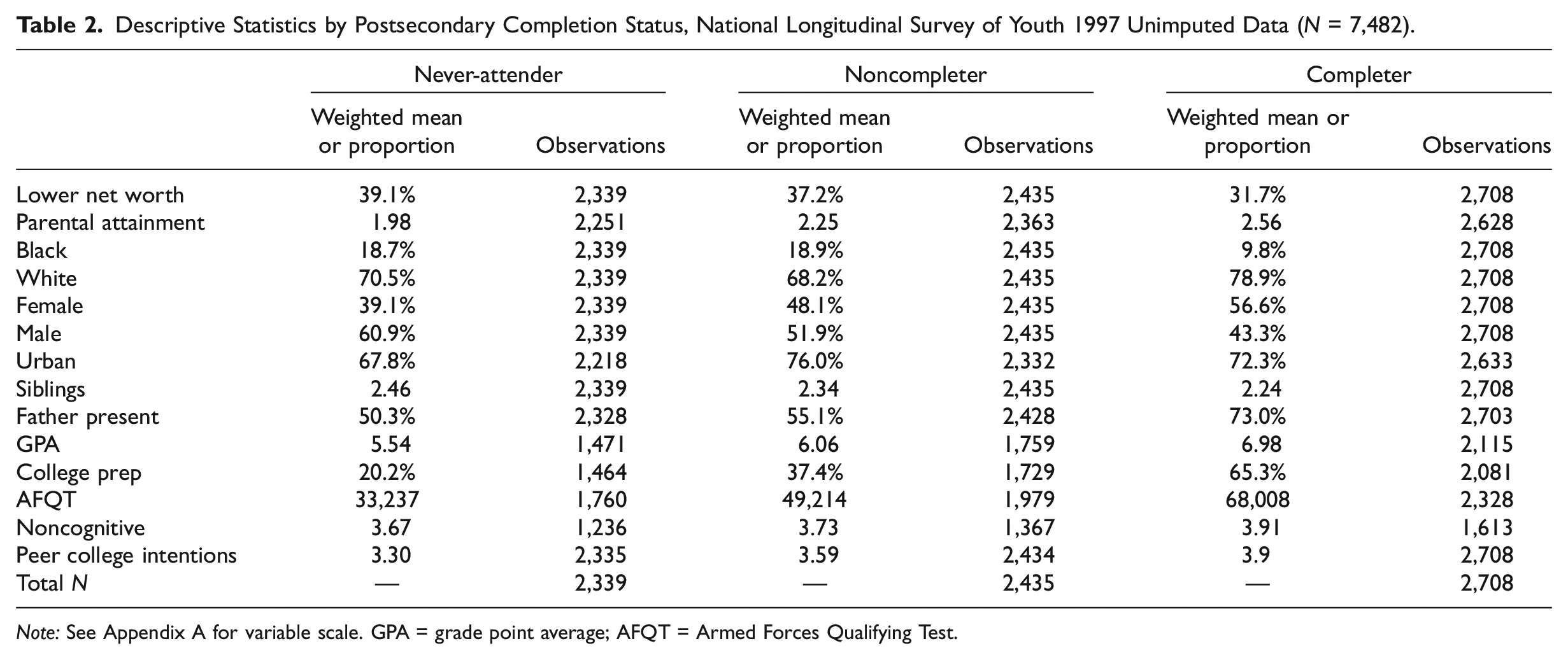
Note: See Appendix A for variable scale. GPA = grade point average; AFQT = Armed Forces Qualifying Test.

Missing observations vary across measures and over time (Table 2). Far fewer observations are available when treatment is observed than were recorded in the initial 1997 survey round (likely due to attrition). Moreover, academic data are limited, particularly college admissions test scores (SAT/ACT). High school grades are stronger predictors of college success than admissions tests (Hoffman and Lowitzki 2005; Noble and Sawyer 2004), and imputing such a large percentage of test score data could introduce substantial bias to effect estimates due to scope (roughly a third of observations include test score data) and because test score availability is skewed by race group. I therefore omit these test scores and rely on Armed Forces Qualifying Test (AFQT) scores instead. To accommodate missing observations in the remainder of the data set, I used the multiple imputation ice package in Stata 14.2 to create 20 imputed data sets.

Dependent and Independent Variables

My dependent variables are logged average income and financial hardship. Logged average income represents each respondent’s average (because income is noisy) annual wages and salary for 2013, 2015, and 2017, logged (with an added $1 constant; I also include a binary indicator for zero reported income) and standardized in 2017 dollars. I constructed a measure of financial hardship by aggregating data from yes/no questions that asked respondents whether they had ever taken out a payday loan or been harassed by a bill collector yearly from 2007 to 2011 and in 2013, 2015, and 2017. To include these variegated information sources in one measure, I created two indicator variables (for ever taking out a payday loan after age 29 and ever facing bill collection harassment after age 29) and summed them, yielding my financial hardship variable. As a sensitivity check, I examined a binary variable indicating ever experiencing any of these situations after age 29; results are robust to this operationalization (see Appendix B).

However, this operationalization likely yields conservative estimates of financial hardship related to noncompletion. First, it only measures financial hardship past age 29. Students frequently stop college for a time, reenter, then stop again (Grosset 1993; Terriquez and Gurantz 2015). Because student loans enter repayment six months (or less, depending on the type of loan) after a student is no longer enrolled, students may experience hardship (e.g., harassment by bill collectors) as part of the process of noncompletion and do so at considerably younger ages than 29. Second, this operationalization of financial hardship measures only payday loan use and collections harassment, which is, arguably, a high bar for defining hardship. Other forms of financial hardship (e.g., late rent or mortgage payments, limited income net of other financial obligations, or damage to one’s credit score) could be meaningful, frequent, and potentially related to student debt yet may not result in payday loan use or collections harassment.

My treatment variable is a multilevel variable in which “never-attenders” are all individuals whose highest degree was a high school diploma or GED, “noncompleters” are all individuals whose highest degree was a high school diploma or GED and who ever enrolled in two- or four-year higher education (enrollment is arrayed annually from 1997 onward in the NLSY97) through the year they turned 29, and “completers” are all individuals who completed an associate’s degree, a bachelor’s degree, or higher in the same period. I compare noncompleters to never-attenders by arranging treatment categories such that D₀ = never-attenders, D₁ = noncompleters, and D₂ = completers. I compare noncompleters to completers by arranging categories such that D₀ = noncompleters, D₁ = completers, and D₂ = never-attenders.

Analytic Approach

Because my questions are causal, my analysis operates within a potential outcomes framework, where treatments are noncompletion and completion and outcomes are income and financial hardship (Winship and Morgan 1999). Many factors could influence whether or not individuals receive treatment. For instance, family background, including caregiver educational attainment and occupation, is influential in status attainment (Blau and Duncan 1967), as are cognitive ability, prior educational achievement, and the expectations of peers (Sewell, Haller, and Portes 1969; Sewell and Hauser 1975). In the returns-to-college literature, analysts typically control for additional factors that are likely to influence selection into treatment, like family structure, family size, family income or net worth, geography, high school curriculum, race, and gender. Figure 1 shows the directed acyclic graph representing these relationships as I theorize and examine them.

Figure 1.

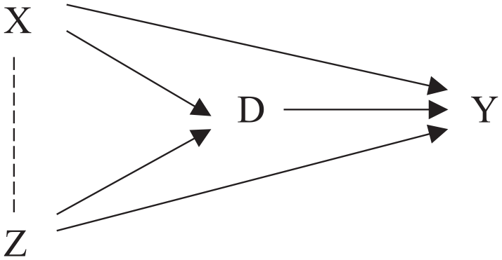
Causal relationships between family background (X), individual characteristics (Z), noncompletion (D), and income (Y).

I estimate the effect of noncompletion on income and financial hardship by modeling these relationships with augmented inverse probability weighting (AIPW), a method common in biostatistics research but comparatively new to the social sciences (see Giani et al. 2020; Glynn and Quinn 2010). AIPW is a parametric technique that estimates regression models in two stages. It first models selection into treatment using logistic regression, which generates a weight (propensity score) for each observation based on its estimated likelihood of receiving treatment. Applying the weights analytically “upweights” both treated and untreated observations with a high likelihood of receiving treatment; that is, if correctly modeled, it will purge observed selection bias from the estimated treatment effect. These weights are applied to a second-stage regression model estimating the effect of treatment on the outcome (see Glynn and Quinn 2010; Rubin and van der Laan 2008; Tan 2010). The procedure closely mirrors inverse probability weighting (IPW); the difference is that the AIPW estimator contains an “augmentation term” that shrinks to zero when both first- and second-stage models are correctly specified and adjusts for bias that can arise when first-stage propensity scores approach their limits (are close to one or zero; Glynn and Quinn 2010:40). In other words, the AIPW estimator retains the attractive properties of the IPW estimator, in that it is doubly robust, but has the advantage of reducing bias in the case of extreme propensity scores and of reducing standard errors.

I implemented AIPW using Stata’s mi estimate and teffects aipw commands.² I modeled selection into treatment using a rich set of covariates indicated by the literature reviewed previously, including measures for family background (parental educational attainment, a binary variable for lower household net worth, father’s presence, and number of siblings), demographics (race, sex, and birth year), geography (a binary variable for living in an urban area), and academic and individual factors (high school grade point average, a binary variable for college-preparatory curricular path, AFQT score, noncognitive score, and peer college-going intentions; see variable details in Appendix A). The first-stage model uses these covariates to estimate treatment weights. The second-stage model estimates the average effect of treatment on outcome net of the covariates and given treatment weights. To contextualize income and hardship outcomes, I also summarize educational debt levels, which are measured at age 30 and reported in 2017 dollars, and assess the mediating role of educational debt in these outcomes.

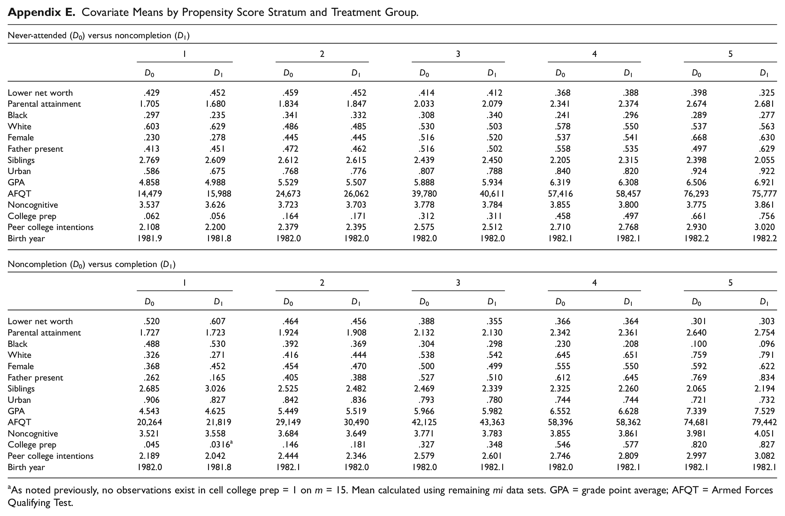
I estimate the treatment effects of noncompletion and completion on income and financial hardship at a population level. To examine effect heterogeneity, I estimate each model in three additional ways. First, I estimate models separately by race, gender, and economic disadvantage (or “lower net worth,” a proxy for class, indicated by the lower household net worth binary variable). Second, I estimate models by intersecting these categories in three dimensions (by race-gender-class). Third, I estimate models by propensity score strata, stratifying observations into quintiles by propensity score, and checking for covariate balance between treated and untreated groups in each stratum (see Appendix E for covariate means). Finally, to visualize observed propensity score heterogeneity, I estimate and graph hierarchical linear models (HLMs), where Level 1 treatment effect estimates are calculated within propensity score strata and then regressed in Level 2 on propensity score stratum rank (Brand and Xie 2010:281; see also Xie, Brand, and Jann 2012).

Model Sensitivity and Selection Bias

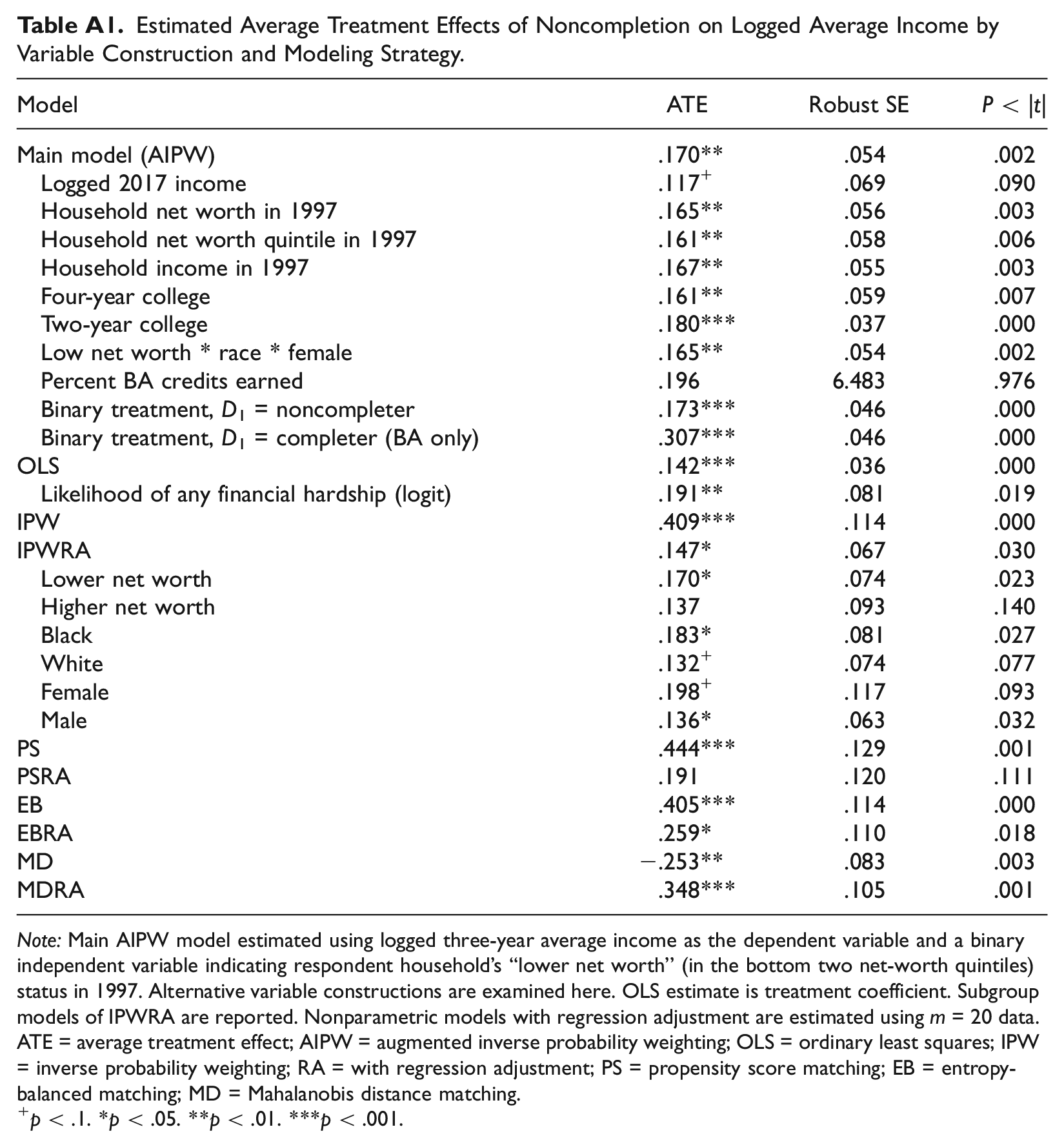
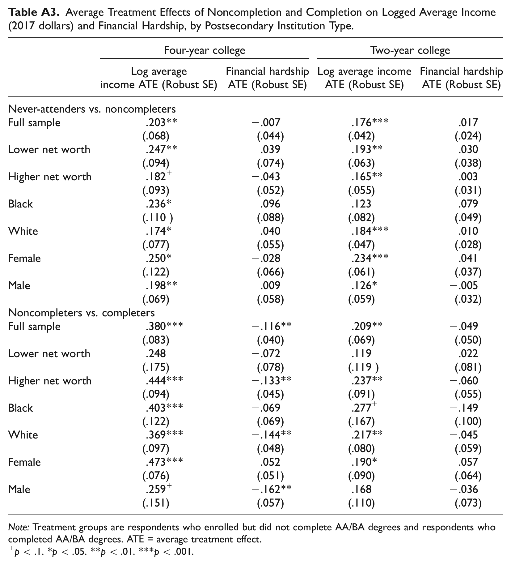
I conducted additional analyses testing whether my main model is sensitive to alternative constructions of the dependent variable, key covariates (e.g., family net worth, attending a two- versus four-year college, or amount of credits accumulated), and covariate interactions. In particular, human capital theory suggests returns to some college should be sensitive to type and amount of postsecondary training. I operationalize this as percent of credits earned toward a bachelor’s degree. However, these data are self-reported and have high missingness, which may bias estimates. I therefore report in Appendix B estimates that include credit attainment as a robustness check but not as part of the main AIPW model. I also report estimates separately by two- and four-year institution in Appendix D; the main effects are broadly robust to this disaggregation. I examined the sensitivity of the main effect to alternative model specifications, including parametric models (ordinary least squares and IPW) and nonparametric models—propensity score matching, entropy-balanced matching, and Mahalanobis distance matching—with and without regression adjustment. Again, the main AIPW model is robust to these alternatives (see Appendix B).

Figure 2 illustrates two potential sources of selection bias common in causal inference: unobserved confounding and endogeneity. In the education literature, a common example of unobserved confounding is noncognitive skill: Individual-level characteristics like perseverance or social and emotional intelligence might shape educational trajectories (Zhou 2019), but measures of noncognitive skill are often unavailable in observational or, especially, administrative data. Here, I adjust for selection bias due to noncognitive skill by developing a measure of it from the NLSY97 data. But this does not preclude other unobserved confounding (as in U₁, Figure 2). Because it is impossible to adjust for all known and unknown unobserved confounders, I conducted supplemental analyses to estimate how sensitive my results may be to this bias. I found that the overall treatment effect estimate obtained by the AIPW model is likely robust to unobserved bias if this bias has a similar effect size as observed biases (see Appendix C).

Figure 2.

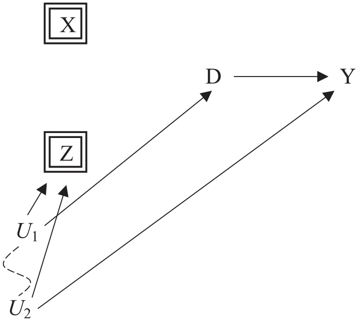
Bias may arise due to the presence of an unobserved confounder (U₁) or conditioning on a collider (Z).

To examine potential endogeneity in this case, it is useful to consider the example of high school curriculum, one of several controlled covariates in the vector Z (see Figure 2). It is probable that high school curriculum is causally affected by other, unobserved variables. For instance, the type of high school (U₁) a student attends (e.g., district-run, charter, parochial) may influence both the school’s curriculum and whether a student attends college. Furthermore, the level of economic development in the area where the high school is located (U₂) may also influence the high school’s curriculum (especially if school funding is tied to local taxes) and may influence a student’s adult earnings if they decide to live in the area where they grew up (as is common). Because a backdoor relationship exists between U₁ and U₂ in this scenario, conditioning on high school curriculum (in vector Z) would distort or induce a spurious relationship between type of high school and economic development that could bias effect estimates (Elwert and Winship 2014:47). The direction and magnitude of any resulting bias is difficult to estimate. However, as with bias due to possible unobserved confounders, I assay its possible scope using estimates for bias introduced by known confounders (see Appendix C) and find the overall treatment effect estimate is robust.

Results

Effects of Noncompletion

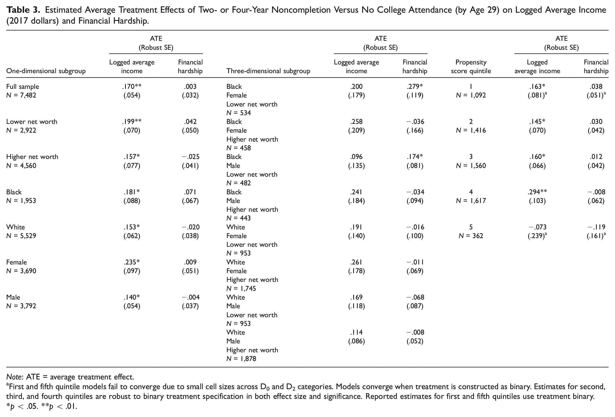
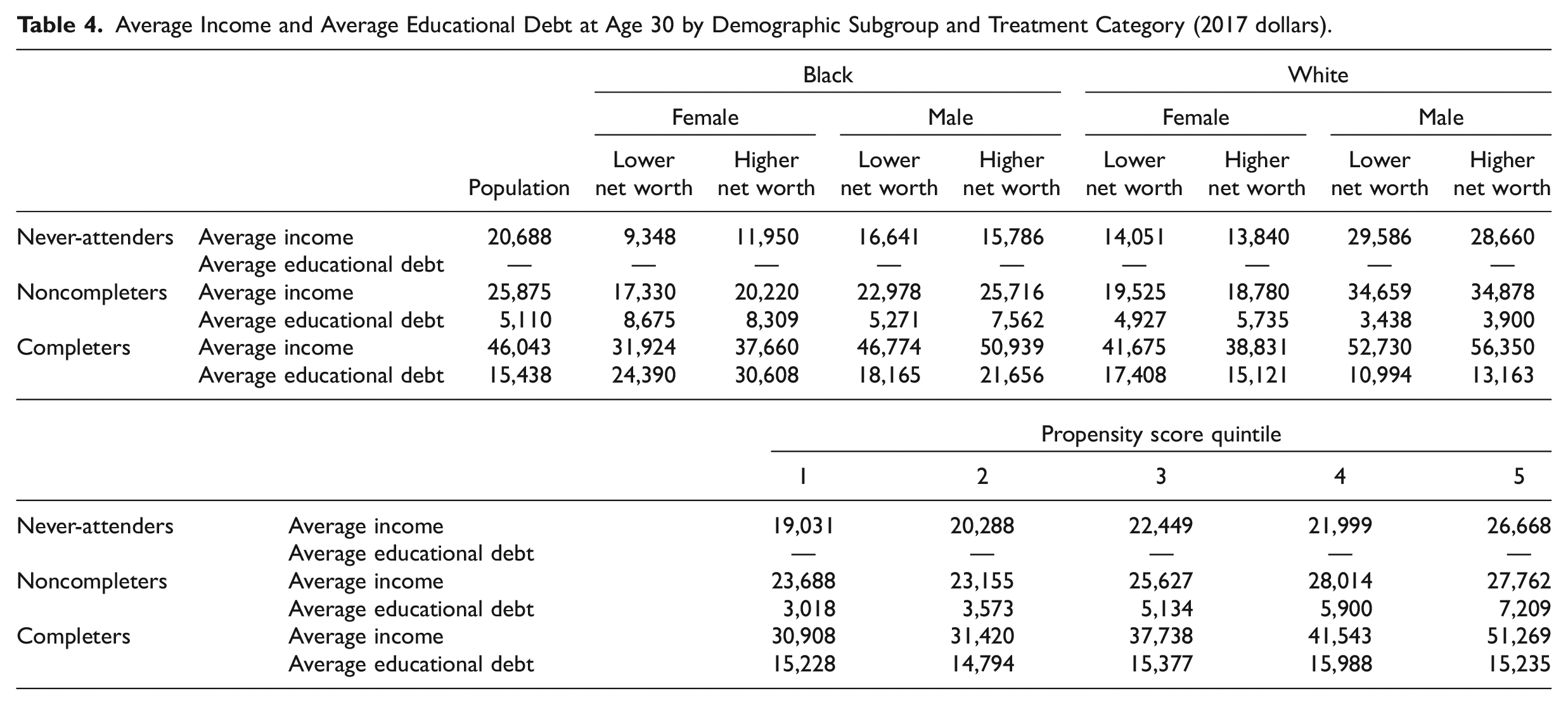
Comparable to prior research, I find that on average, noncompletion increases annual income by around 17 percent compared to no college (see Table 3). Despite these income returns, noncompletion has a negligible and statistically insignificant average effect on financial hardship. This is perhaps not surprising given that, as Table 4 shows, noncompleters hold an average of just over $5,100 in educational debt.

Table 3.

Estimated Average Treatment Effects of Two- or Four-Year Noncompletion Versus No College Attendance (by Age 29) on Logged Average Income (2017 dollars) and Financial Hardship.

One-dimensional subgroup	ATE(Robust SE)		Three-dimensional subgroup	ATE(Robust SE)		Propensity score quintile	ATE(Robust SE)
One-dimensional subgroup	Logged average income	Financial hardship	Three-dimensional subgroup	Logged average income	Financial hardship	Propensity score quintile	Logged average income	Financial hardship
Full sample N = 7,482	.170** (.054)	.003 (.032)	Black Female Lower net worth N = 534	.200 (.179)	.279* (.119)	1 N = 1,092	.163* (.081)^a	.038 (.051)^a
Lower net worth N = 2,922	.199** (.070)	.042 (.050)	Black Female Higher net worth N = 458	.258 (.209)	−.036 (.166)	2 N = 1,416	.145* (.070)	.030 (.042)
Higher net worth N = 4,560	.157* (.077)	−.025 (.041)	Black Male Lower net worth N = 482	.096 (.135)	.174* (.081)	3 N = 1,560	.160* (.066)	.012 (.042)
Black N = 1,953	.181* (.088)	.071 (.067)	Black Male Higher net worth N = 443	.241 (.184)	−.034 (.094)	4 N = 1,617	.294** (.103)	−.008 (.062)
White N = 5,529	.153* (.062)	−.020 (.038)	White Female Lower net worth N = 953	.191 (.140)	−.016 (.100)	5 N = 362	−.073 (.239)^a	−.119 (.161)^a
Female N = 3,690	.235* (.097)	.009 (.051)	White Female Higher net worth N = 1,745	.261 (.178)	−.011 (.069)
MaleN = 3,792	.140* (.054)	−.004(.037)	WhiteMaleLower net worthN = 953	.169(.118)	−.068(.087)
			WhiteMaleHigher net worthN = 1,878	.114(.086)	−.008(.052)

Note: ATE = average treatment effect.

First and fifth quintile models fail to converge due to small cell sizes across D₀ and D₂ categories. Models converge when treatment is constructed as binary. Estimates for second, third, and fourth quintiles are robust to binary treatment specification in both effect size and significance. Reported estimates for first and fifth quintiles use treatment binary.

p < .05. **p < .01.

Table 4.

Average Income and Average Educational Debt at Age 30 by Demographic Subgroup and Treatment Category (2017 dollars).

		Population	Black				White
			Female		Male		Female		Male
			Lower net worth	Higher net worth	Lower net worth	Higher net worth	Lower net worth	Higher net worth	Lower net worth	Higher net worth
Never-attenders	Average income	20,688	9,348	11,950	16,641	15,786	14,051	13,840	29,586	28,660
Never-attenders	Average educational debt	—	—	—	—	—	—	—	—	—
Noncompleters	Average income	25,875	17,330	20,220	22,978	25,716	19,525	18,780	34,659	34,878
Noncompleters	Average educational debt	5,110	8,675	8,309	5,271	7,562	4,927	5,735	3,438	3,900
Completers	Average income	46,043	31,924	37,660	46,774	50,939	41,675	38,831	52,730	56,350
Completers	Average educational debt	15,438	24,390	30,608	18,165	21,656	17,408	15,121	10,994	13,163
				Propensity score quintile
				1	2		3		4	5
Never-attenders	Average income			19,031	20,288		22,449		21,999	26,668
Never-attenders	Average educational debt			—	—		—		—	—
Noncompleters	Average income			23,688	23,155		25,627		28,014	27,762
Noncompleters	Average educational debt			3,018	3,573		5,134		5,900	7,209
Completers	Average income			30,908	31,420		37,738		41,543	51,269
Completers	Average educational debt			15,228	14,794		15,377		15,988	15,235

When examined by ascribed categories like race, class, and gender, these effects appear somewhat heterogeneous. Income returns to noncompletion are greater among Black people, women, and people from lower net-worth families (and, as the three-dimensional subgroup column of Table 3 shows, are greater but not statistically significant among lower net-worth Black women and Black respondents and white women who come from higher net-worth families). Financial hardship, on the other hand, increases among Black respondents from lower net-worth families.

When examined by likelihood of attempting but not completing college (by propensity score strata), the effects of noncompletion appear differently heterogeneous. Income effect estimates are greatest in the first and fourth propensity score quintiles and lower in the second, third, and fifth quintiles (although the fifth quintile estimate is statistically insignificant at p > .05). Noncompletion has uneven and small effects on financial hardship by propensity score strata, but none of these estimates are statistically significant.

Effects of Completion

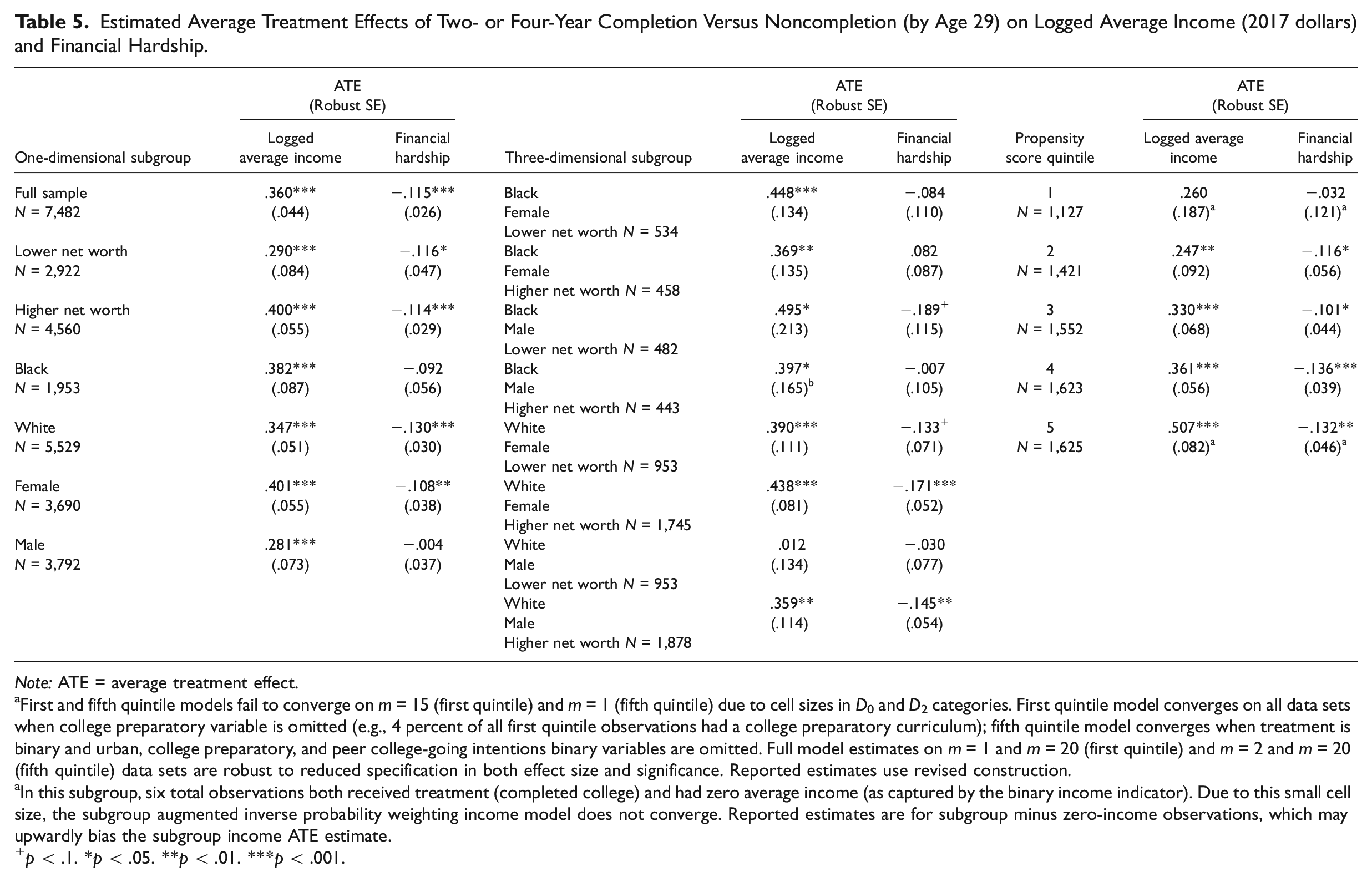
In contrast, the effects of completion are larger and more often significant across subgroups (see Table 5). On average, completion increases annual income by around 36 percent, compared to some college. Completion also decreases the incidence of financial hardship by about 27 percent (mean financial hardship incidence among noncompleters is .432). Completers average lower financial hardship, despite taking out considerably more educational debt, than noncompleters ($15,438, on average, see Table 4).

Table 5.

Estimated Average Treatment Effects of Two- or Four-Year Completion Versus Noncompletion (by Age 29) on Logged Average Income (2017 dollars) and Financial Hardship.

One-dimensional subgroup	ATE(Robust SE)		Three-dimensional subgroup	ATE(Robust SE)		Propensity score quintile	ATE(Robust SE)
One-dimensional subgroup	Logged average income	Financial hardship	Three-dimensional subgroup	Logged average income	Financial hardship	Propensity score quintile	Logged average income	Financial hardship
Full sampleN = 7,482	.360*** (.044)	−.115*** (.026)	BlackFemaleLower net worth N = 534	.448*** (.134)	−.084 (.110)	1N = 1,127	.260 (.187)^a	−.032 (.121)^a
Lower net worthN = 2,922	.290*** (.084)	−.116* (.047)	BlackFemaleHigher net worth N = 458	.369** (.135)	.082 (.087)	2N = 1,421	.247** (.092)	−.116* (.056)
Higher net worthN = 4,560	.400*** (.055)	−.114*** (.029)	BlackMaleLower net worth N = 482	.495* (.213)	−.189⁺ (.115)	3N = 1,552	.330*** (.068)	−.101* (.044)
BlackN = 1,953	.382*** (.087)	−.092 (.056)	BlackMaleHigher net worth N = 443	.397* (.165)^b	−.007 (.105)	4N = 1,623	.361*** (.056)	−.136*** (.039)
WhiteN = 5,529	.347*** (.051)	−.130*** (.030)	WhiteFemaleLower net worth N = 953	.390*** (.111)	−.133⁺ (.071)	5N = 1,625	.507*** (.082)^a	−.132** (.046)^a
FemaleN = 3,690	.401*** (.055)	−.108** (.038)	WhiteFemaleHigher net worth N = 1,745	.438*** (.081)	−.171*** (.052)
MaleN = 3,792	.281*** (.073)	−.004 (.037)	WhiteMaleLower net worth N = 953	.012 (.134)	−.030 (.077)
			WhiteMaleHigher net worth N = 1,878	.359** (.114)	−.145** (.054)

Note: ATE = average treatment effect.

First and fifth quintile models fail to converge on m = 15 (first quintile) and m = 1 (fifth quintile) due to cell sizes in D₀ and D₂ categories. First quintile model converges on all data sets when college preparatory variable is omitted (e.g., 4 percent of all first quintile observations had a college preparatory curriculum); fifth quintile model converges when treatment is binary and urban, college preparatory, and peer college-going intentions binary variables are omitted. Full model estimates on m = 1 and m = 20 (first quintile) and m = 2 and m = 20 (fifth quintile) data sets are robust to reduced specification in both effect size and significance. Reported estimates use revised construction.

In this subgroup, six total observations both received treatment (completed college) and had zero average income (as captured by the binary income indicator). Due to this small cell size, the subgroup augmented inverse probability weighting income model does not converge. Reported estimates are for subgroup minus zero-income observations, which may upwardly bias the subgroup income ATE estimate.

p < .1. *p < .05. **p < .01. ***p < .001.

Again, effect estimates for completion vary by ascribed subgroup and by propensity score stratum. Compared to noncompleters, postsecondary graduates who are Black or women average greater income returns (compared to white people or men), particularly Black women, Black men, and white women from lower net-worth backgrounds.³ However, white women from higher net-worth backgrounds also average some of the highest returns to completion. White women and Black men from lower net-worth backgrounds also see significant reduction in financial hardship, but the greatest estimated decrease in financial hardship accrues to white women from higher net-worth families.

Income variation is somewhat different when examined by likelihood of completing college, revealing a U-shaped pattern: Income returns to completion are greater among those least likely and most likely to complete their degrees (this is consistent with prior research; see Cheng et al. 2021). Financial hardship, however, is patterned more linearly: Completion has very little (if any) effect on financial hardship among individuals least likely to complete (in the first quintile) and yields incrementally greater reductions in financial hardship as the likelihood of completion increases.

Significance Testing

A statistically significant point estimate for a given subgroup does not necessarily indicate that point estimates for various subgroups are significantly different from each other. To test whether ascribed subgroup effect estimates differ from one another in statistically significant ways, I pooled comparison groups and interacted indicators for subgroup membership with treatment. The significance of the interaction term indicates the significance of average treatment effect (ATE) differences between the two groups. Constraints of teffects aipw make it infeasible to directly apply this strategy using Stata, but I performed a proxy test by first verifying that IPW yields similar effect estimates as AIPW and then manually performing two-stage regression with treatment interaction terms in the second stage. For demographic subgroups, differences in subgroup ATEs are not statistically significant. A power analysis, however, shows that most subgroup sample sizes are insufficiently large to rule out a Type II error.

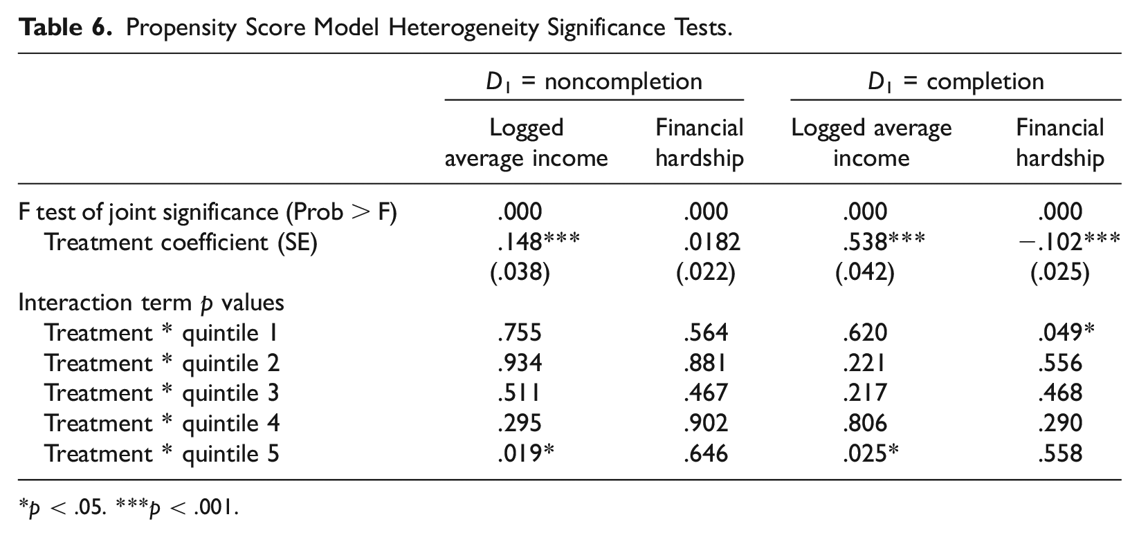
For propensity score strata, differences in subgroup estimates may be tested directly using HLM models; results are significant for noncompletion in the fifth quintile (on income) and for completion in the fifth (on income) and first (on financial hardship) quintiles (see Table 6). Figure 3 shows this variation in an HLM graph. I also conducted F tests comparing propensity score model fit with and without stratum-level dummy variables; in each case, model fit is improved by including strata dummies.

Table 6.

Propensity Score Model Heterogeneity Significance Tests.

	D₁ = noncompletion		D₁ = completion
	Logged average income	Financial hardship	Logged average income	Financial hardship
F test of joint significance (Prob > F)	.000	.000	.000	.000
Treatment coefficient (SE)	.148*** (.038)	.0182 (.022)	.538*** (.042)	−.102*** (.025)
Interaction term p values
Treatment * quintile 1	.755	.564	.620	.049*
Treatment * quintile 2	.934	.881	.221	.556
Treatment * quintile 3	.511	.467	.217	.468
Treatment * quintile 4	.295	.902	.806	.290
Treatment * quintile 5	.019*	.646	.025*	.558

p < .05. ***p < .001.

Figure 3.

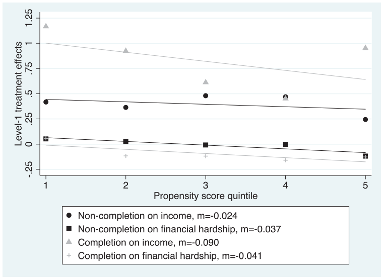
Hierarchical linear model of effects of noncompletion and completion on economic outcomes by propensity score strata.

The Mediating Role of Educational Debt

To understand the role educational debt plays in these findings, particularly regarding financial hardship, I conducted a basic mediation analysis comparing ATE estimates between main AIPW models that exclude (total effect model) and include (direct effect model) total educational debt at age 30 in the second-stage regression. When educational debt is controlled, noncompletion reduces financial hardship, on average, and financial hardship caused by noncompletion among Black women and men from low-income families appears completely attenuated, becoming negative and statistically insignificant (see Table 7). In the main model, completion is estimated to reduce financial hardship, and this effect increases 15 percent when educational debt is controlled. Educational debt also mediates the relationship between completion and income and may mediate the relationship between noncompletion and income by an even larger magnitude (but this estimate is not significant).

Table 7.

Treatment Effect Mediation by Educational Debt at Age 30.

		D1 = noncompletion				D1 = completion
		Total effect (Robust SE)	Direct effect (Robust SE)	Difference	Percentage difference	Total effect (Robust SE)	Direct effect (Robust SE)	Difference	Percentage difference
AIPW main	Logged average income (2017 dollars)	.165** (.054)	.314 (.280)	.149	47.52	.360*** (.045)	.343*** (.045)	−.017	−4.86
AIPW main	Financial hardship	.003 (.032)	−.165⁺ (.087)	−.168	101.69	−.115*** (.026)	−.136*** (.027)	−.021	15.38
Black Female Lower net worth	Logged average income (2017 dollars)	.211 (.182)	.119 (.316)	−.093	−78.26	.457*** (.136)	.412** (.137)	−.045	−10.95
Black Female Lower net worth	Financial hardship	.269* (.113)	−.071 (.259)	−.340	475.95	−.088 (.110)	−.107 (.110)	−.019	17.38
Black Male Lower net worth	Logged average income (2017 dollars)	.099 (.136)	−3.668* (1.663)	−3.76622	102.69	.500* (.211)	.435⁺ (.221)	−.064	−14.79
Black Male Lower net worth	Financial hardship	.175* (.080)	−.057 (2.503)	−.231	407.23	−.213⁺ (.117)	−.336** (.113)	−.123	36.69

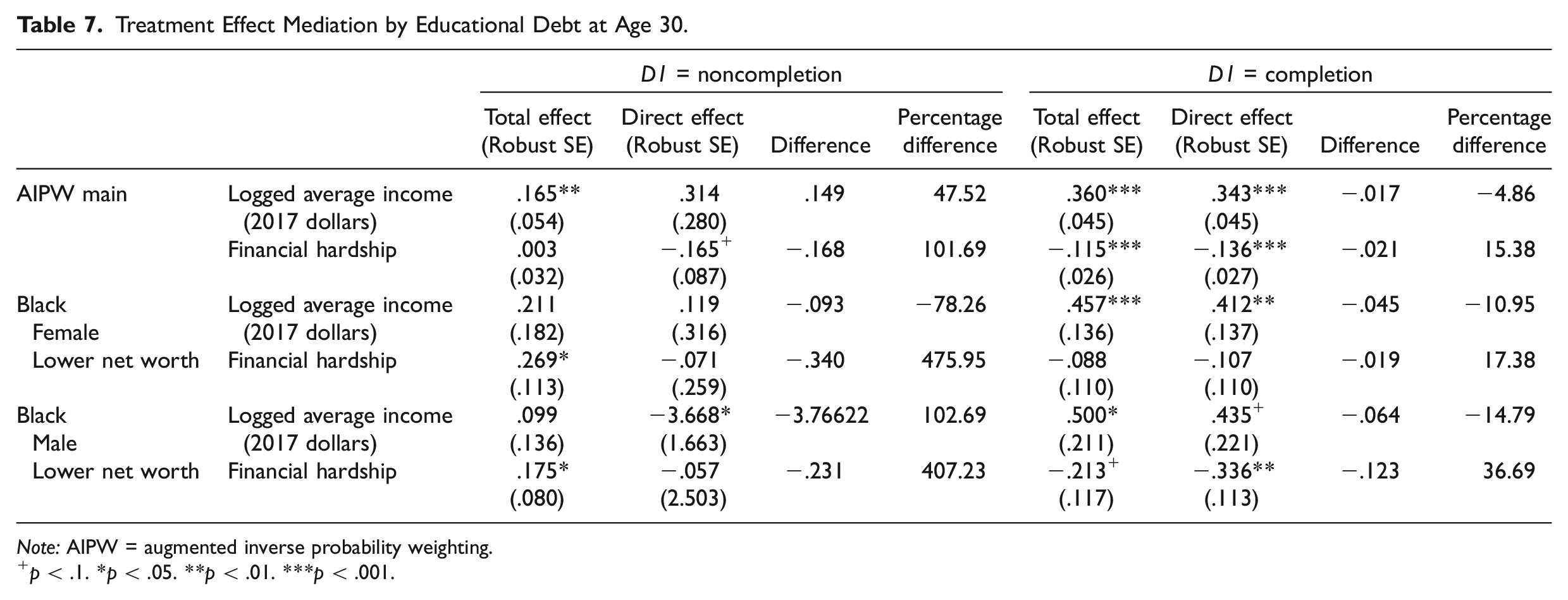
Note: AIPW = augmented inverse probability weighting.

p < .1. *p < .05. **p < .01. ***p < .001.

Discussion

What do these results mean for reproduction and equalization theories of higher education? The average U.S. millennial who started but did not finish college earns more money than they would have if they never attended. This supports human capital and signaling hypotheses. Yet noncompletion has a negligible and statistically insignificant effect on financial hardship (as operationalized by payday lending and collections harassment) because of educational debt: Net of student debt, the average person with some college would have experienced less financial hardship as a result of attending college. But certain groups (e.g., Black women and Black men from lower net-worth families) both earn more income and experience greater financial hardship as a result of some college, suggesting noncompletion may help reproduce inequality among disadvantaged groups. Controlling for educational debt attenuates this subgroup effect on financial hardship.

In contrast, and again at a population level, college completion has an equalizing effect on financial position: Completion raises income and reduces financial hardship. On average, individuals who exited with “some college” would have been better off financially had they completed their degrees (as the credential hypothesis would expect). Thus, individuals may be better off, on average, in terms of income and financial hardship as a result of college completion (a type of equalization) but are no better off, on average, in terms of financial hardship as a result of college noncompletion (a type of reproduction). Higher education, in this analysis, has dual and contrary effects at the population level—an observation that emerges when noncompletion is studied against both of its counterfactuals simultaneously.

However, these effects sometimes vary within the population. For instance, the effect of completion compared to some college has a somewhat equalizing effect on income for individuals least likely to finish college and appears to most benefit members of ascribed categories that are associated with socioeconomic disadvantage (i.e., Black people from lower net-worth backgrounds) in terms of income. Yet the U-shaped pattern in income returns to completion across propensity score strata observed in Figure 3 complicates the equalization hypothesis: Individuals with the lowest and highest likelihood of completing college gain the most from doing so (perhaps a combined effect of a lower baseline income among people least likely to complete and the fact that people most likely to complete may also be most likely to attend highly selective institutions that yield greater socioeconomic returns for their graduates [Zhou 2019], although this is speculative). In terms of financial hardship, college completion may have an average equalizing effect among specific ascribed subgroups but a reproductive effect at the level of individual likelihood of college completion: The more likely an individual is to complete college, the greater their reduction in financial hardship as a result of graduating.

However, in this case, evidence for effect heterogeneity by propensity score strata is stronger than evidence for effect heterogeneity by ascribed subgroup, which may be the result of a true absence of effect difference across ascribed subgroups but may also result from the nature of the NLSY97 data. Complementary analyses using larger, administrative data sets could help clarify this question. Other limitations include possible variation due to unobserved but potentially salient differences, such as undergraduate major or course of study, which is uncontrolled here (but see Zeidenberg et al. 2015), or institutional factors like selectivity or public versus private status. Importantly, the analysis provides preliminary evidence that the financial benefits of greater income following both noncompletion and completion are mediated and sometimes erased by educational debt. Future analyses, however, should examine this further, studying educational debt at different points in the life course and evaluating how its mediating effects may change over time and within the population (an analysis limited by sample size here). This is particularly salient given that student debt default rates vary by race, class, gender, and institution type (see Postsecondary Value Commission 2021:10).

Attending to Ambiguity

Ambiguity emerges at several points in the data and merits examination and even theorization. For instance, who benefits most from higher education seems contradictory: I find elements of both positive selection (e.g., less financial hardship among people more likely to complete college) and negative selection (e.g., greater income returns among less advantaged ascribed groups and greater or U-shaped income returns to completion among those least likely to complete). Earning a college degree can yield substantial financial benefits, but failing to complete can, in some cases, lead to more financial hardship than people would otherwise experience. This again supports (or contradicts) elements of both the equalization and reproduction theses.

One could approach this ambiguity as an object of analysis (Deener 2017; Lamont, Beljean, and Clair 2014:584–85). These data and the conflicting literature on the social consequences of higher education suggest that two things are simultaneously true: For completers and noncompleters, a college education yields socioeconomic returns for some and reproduces inequality for others. Perhaps, in a society that many argue is predicated on inequality and deeply invested in a cultural mythology of meritocracy (e.g., Groeger 2021), higher education functions exactly as it needs to: It does not straightforwardly reproduce socioeconomic status, because doing so would undermine contemporary meritocratic ideals, but neither does it function as the “great equalizer,” because doing so would flatten a social order that arguably depends on social inequalities to operate (Bourdieu and Passeron [(1970) 2000] make a similar argument).

How, then, does higher education yield both socioeconomic returns and social reproduction? At the individual level, college likely seems risky but perhaps worth it—because it appears that people can reap meaningful rewards. Similar actions by similar individuals can lead to different results, but it can be difficult for individuals to perceive why their outcomes differ without relying on narratives of individual merit that obscure structural forces. Social means of meaningful action become separated from social ends or outcomes—a condition that obscures from social agents the mechanisms of this separation (Deener 2017:369). In other words, the relevant ambiguity may be both structural (in the sense that both equalization and reproduction seem to take place) and subjective (in that effect heterogeneity may create ambiguity at the level of social action). Qualitative data could illuminate processes of means-ends separation, that is, the production of ambiguity, in the context of college noncompletion more usefully than can the present, quantitative data.

Yet an ambiguity-as-object hypothesis is dissatisfying in several respects. A considerable benefit of both equalization and reproduction hypotheses is they support relatively clear ethical imaginaries: If college delivers meaningful returns to those who most need them, then an obvious way to work toward greater equity is to support college access and completion for those individuals. If college simply reproduces inequality, then those working toward equity must radically reform (or, some might say, abandon) the equalizing project of U.S. higher education as it has been popularly understood.

But if U.S. higher education is at base more ambiguous in both its aims and its ends, projects that would use higher education as a vehicle for equity must necessarily grapple with that ambiguity. This point is underlined in the Postsecondary Value Commission’s 2021 report, which advocates for a wider plurality of measures of the economic returns to higher education. Policymakers often assume homogeneous schooling effects; this article adds to a growing body of research that cautions against that approach (e.g., Brand et al. 2014; Postsecondary Value Commission 2021). This analysis further indicates that disadvantaged people with some college could benefit considerably from relatively modest amounts of student debt forgiveness.

Conclusions

Debates about the social function of higher education—its equalizing or reproductive possibilities—frequently focus on the experiences of college completers. In the U.S. context, I argue it is useful to broaden these debates in at least three ways: (1) by centering the experiences of the nearly half of all U.S. college students who exit higher education without a degree, (2) by examining noncompletion simultaneously against its two counterfactuals (never attending college and college completion), and (3) by considering other relevant outcomes, such as financial hardship. Such broadening is particularly useful given the paired realities of persistently low college completion rates and the recent transformations of higher education, including greater college access, escalating costs, and runaway student debt levels.

Individuals and policymakers interested in whether young people should attempt a college education in the current U.S. postsecondary landscape should draw both hope and caution from this analysis. It shows that college is risky in the medium term: Many people who aspire to earn a degree do not complete their education, yet they acquire substantial debt and sometimes experience more financial hardship in early adulthood, particularly if they are from lower net-worth backgrounds and Black (what happens over the longer life course bears further investigation). Still, attempting some college is associated with greater income levels among some groups, and most noncompleters would have earned more money and experienced less financial hardship if they had completed college, despite taking out more debt. For college-bound individuals, advocates, lawmakers, and higher-education administrators, the issue of college completion should remain a central concern.

Footnotes

Appendix A. Descriptions of Family and Individual Variables

Appendix B. Model Sensitivity

Table A1.

Estimated Average Treatment Effects of Noncompletion on Logged Average Income by Variable Construction and Modeling Strategy.

Model	ATE	Robust SE	P < \|t\|
Main model (AIPW)	.170**	.054	.002
Logged 2017 income	.117⁺	.069	.090
Household net worth in 1997	.165**	.056	.003
Household net worth quintile in 1997	.161**	.058	.006
Household income in 1997	.167**	.055	.003
Four-year college	.161**	.059	.007
Two-year college	.180***	.037	.000
Low net worth * race * female	.165**	.054	.002
Percent BA credits earned	.196	6.483	.976
Binary treatment, D₁ = noncompleter	.173***	.046	.000
Binary treatment, D₁ = completer (BA only)	.307***	.046	.000
OLS	.142***	.036	.000
Likelihood of any financial hardship (logit)	.191**	.081	.019
IPW	.409***	.114	.000
IPWRA	.147*	.067	.030
Lower net worth	.170*	.074	.023
Higher net worth	.137	.093	.140
Black	.183*	.081	.027
White	.132⁺	.074	.077
Female	.198⁺	.117	.093
Male	.136*	.063	.032
PS	.444***	.129	.001
PSRA	.191	.120	.111
EB	.405***	.114	.000
EBRA	.259*	.110	.018
MD	−.253**	.083	.003
MDRA	.348***	.105	.001

Note: Main AIPW model estimated using logged three-year average income as the dependent variable and a binary independent variable indicating respondent household’s “lower net worth” (in the bottom two net-worth quintiles) status in 1997. Alternative variable constructions are examined here. OLS estimate is treatment coefficient. Subgroup models of IPWRA are reported. Nonparametric models with regression adjustment are estimated using m = 20 data. ATE = average treatment effect; AIPW = augmented inverse probability weighting; OLS = ordinary least squares; IPW = inverse probability weighting; RA = with regression adjustment; PS = propensity score matching; EB = entropy-balanced matching; MD = Mahalanobis distance matching.

p < .1. *p < .05. **p < .01. ***p < .001.

Appendix C. Sensitivity Analysis for Unobserved Confounding and Endogeneity

The magnitude and direction of bias due to unobserved confounders and endogeneity are impossible to know. However, estimating selection biases for observed confounders can create a set of proxy estimates for potential bias due to unobserved confounders or biasing pathways. In other words, it is possible to estimate how strongly a hypothetical unobserved confounder or controlled collider would bias treatment effect estimates if it biased selection as strongly as a given observed confounder did. Zhou (2019:32–34) shows that selection bias for each observed confounder may be estimated by taking the product of its coefficients in two separate models that are (1) unweighted and (2) weighted for selection. Following this approach, Table A2 gives the estimated bias and adjusted average treatment effect estimate for each of the observed confounders in second-stage regression of the main augmented inverse probability weighting model. Most biasing effects are very small or negligible. The largest biasing effects would result if the biasing effect of an unobserved confounder were as strong as the selection bias of the covariates for being white (upward bias) or female (downward bias) or for father’s presence in childhood (downward bias). In none of these cases is the adjusted estimated effect of noncompletion driven to zero or below.

Appendix D. Treatment Effects by Institution Type

Table A3.

Average Treatment Effects of Noncompletion and Completion on Logged Average Income (2017 dollars) and Financial Hardship, by Postsecondary Institution Type.

	Four-year college		Two-year college
	Log average income ATE (Robust SE)	Financial hardship ATE (Robust SE)	Log average income ATE (Robust SE)	Financial hardship ATE (Robust SE)
Never-attenders vs. noncompleters
Full sample	.203** (.068)	−.007 (.044)	.176*** (.042)	.017 (.024)
Lower net worth	.247** (.094)	.039 (.074)	.193** (.063)	.030 (.038)
Higher net worth	.182⁺ (.093)	−.043 (.052)	.165** (.055)	.003 (.031)
Black	.236* (.110 )	.096 (.088)	.123 (.082)	.079 (.049)
White	.174* (.077)	−.040 (.055)	.184*** (.047)	−.010 (.028)
Female	.250* (.122)	−.028 (.066)	.234*** (.061)	.041 (.037)
Male	.198** (.069)	.009 (.058)	.126* (.059)	−.005 (.032)
Noncompleters vs. completers
Full sample	.380*** (.083)	−.116** (.040)	.209** (.069)	−.049 (.050)
Lower net worth	.248 (.175)	−.072 (.078)	.119 (.119 )	.022 (.081)
Higher net worth	.444*** (.094)	−.133** (.045)	.237** (.091)	−.060 (.055)
Black	.403*** (.122)	−.069 (.069)	.277⁺ (.167)	−.149 (.100)
White	.369*** (.097)	−.144** (.048)	.217** (.080)	−.045 (.059)
Female	.473*** (.076)	−.052 (.051)	.190* (.090)	−.057 (.064)
Male	.259⁺ (.151)	−.162** (.057)	.168 (.110)	−.036 (.073)

Note: Treatment groups are respondents who enrolled but did not complete AA/BA degrees and respondents who completed AA/BA degrees. ATE = average treatment effect.

p < .1. *p < .05. **p < .01. ***p < .001.

Appendix E. Covariate Means by Propensity Score Stratum and Treatment Group

Never-attended (D₀) versus noncompletion (D₁)
	1		2		3		4		5
	D ₀	D ₁	D ₀	D ₁	D ₀	D ₁	D ₀	D ₁	D ₀	D ₁
Lower net worth	.429	.452	.459	.452	.414	.412	.368	.388	.398	.325
Parental attainment	1.705	1.680	1.834	1.847	2.033	2.079	2.341	2.374	2.674	2.681
Black	.297	.235	.341	.332	.308	.340	.241	.296	.289	.277
White	.603	.629	.486	.485	.530	.503	.578	.550	.537	.563
Female	.230	.278	.445	.445	.516	.520	.537	.541	.668	.630
Father present	.413	.451	.472	.462	.516	.502	.558	.535	.497	.629
Siblings	2.769	2.609	2.612	2.615	2.439	2.450	2.205	2.315	2.398	2.055
Urban	.586	.675	.768	.776	.807	.788	.840	.820	.924	.922
GPA	4.858	4.988	5.529	5.507	5.888	5.934	6.319	6.308	6.506	6.921
AFQT	14,479	15,988	24,673	26,062	39,780	40,611	57,416	58,457	76,293	75,777
Noncognitive	3.537	3.626	3.723	3.703	3.778	3.784	3.855	3.800	3.775	3.861
College prep	.062	.056	.164	.171	.312	.311	.458	.497	.661	.756
Peer college intentions	2.108	2.200	2.379	2.395	2.575	2.512	2.710	2.768	2.930	3.020
Birth year	1981.9	1981.8	1982.0	1982.0	1982.0	1982.0	1982.1	1982.1	1982.2	1982.2
Noncompletion (D₀) versus completion (D₁)
	1		2		3		4		5
	D ₀	D ₁	D ₀	D ₁	D ₀	D ₁	D ₀	D ₁	D ₀	D ₁
Lower net worth	.520	.607	.464	.456	.388	.355	.366	.364	.301	.303
Parental attainment	1.727	1.723	1.924	1.908	2.132	2.130	2.342	2.361	2.640	2.754
Black	.488	.530	.392	.369	.304	.298	.230	.208	.100	.096
White	.326	.271	.416	.444	.538	.542	.645	.651	.759	.791
Female	.368	.452	.454	.470	.500	.499	.555	.550	.592	.622
Father present	.262	.165	.405	.388	.527	.510	.612	.645	.769	.834
Siblings	2.685	3.026	2.525	2.482	2.469	2.339	2.325	2.260	2.065	2.194
Urban	.906	.827	.842	.836	.793	.780	.744	.744	.721	.732
GPA	4.543	4.625	5.449	5.519	5.966	5.982	6.552	6.628	7.339	7.529
AFQT	20,264	21,819	29,149	30,490	42,125	43,363	58,396	58,362	74,681	79,442
Noncognitive	3.521	3.558	3.684	3.649	3.771	3.783	3.855	3.861	3.981	4.051
College prep	.045	.0316^a	.146	.181	.327	.348	.546	.577	.820	.827
Peer college intentions	2.189	2.042	2.444	2.346	2.579	2.601	2.746	2.809	2.997	3.082
Birth year	1982.0	1981.8	1982.1	1982.0	1982.0	1982.1	1982.0	1982.1	1982.1	1982.1

As noted previously, no observations exist in cell college prep = 1 on m = 15. Mean calculated using remaining mi data sets. GPA = grade point average; AFQT = Armed Forces Qualifying Test.

Acknowledgements

The author sincerely thanks Michael Burawoy, David Harding, Jason Houle, Sandra Smith, Sam Lucas, Carmen Brick, Aya Fabros, Shannon Ikebe, Andrew Jaeger, Thomas Peng, the members of the 2021–2022 Gardner Seminar at Berkeley’s Center for Studies in Higher Education, and several anonymous reviewers for their invaluable support and excellent feedback on earlier iterations of this article. The article was also improved by presentations and commentators at the annual meetings of the American Sociological Association, the Society for the Advancement of Socio-Economics, the Sociology of Education Association, the California Sociological Association, and the Eastern Sociological Society.

Research Ethics

The conduct of this research is consistent with the ethical standards described in the 1964 Declaration of Helsinki. This research does not constitute human subjects research.

ORCID iD

Sarah S.C. Payne

Notes

Author Biography

Sarah S.C. Payne is a PhD candidate in sociology at UC-Berkeley. She studies racial inequality, stratification, higher education, debt, subjectivity, and culture using quantitative and qualitative methods.

References

Armstrong

Elizabeth A.

Hamilton

Laura T.

. 2013. Paying for the Party: How College Maintains Inequality. Cambridge, MA: Harvard University Press.

Becker

Gary

. 1964. Human Capital: A Theoretical and Empirical Analysis, with Special Reference to Education. Chicago, IL: University of Chicago Press.

Blau

Peter M.

Duncan

Otis Dudley

. 1967. The American Occupational Structure. New York, NY: John Wiley & Sons.

Bourdieu

Pierre

Passeron

Jean-Claude

. [1970] 2000. Reproduction in Education, Society, and Culture. London: Sage Publications.

Brand

Jennie E.

Pfeffer

Fabian

Goldrick-Rab

Sara

. 2014. “The Community College Effect Revisited: The Importance of Attending to Heterogeneity and Complex Counterfactuals.” Sociological Science 1:448–65.

Brand

Jennie E.

Xie

. 2010. “Who Benefits Most from College? Evidence for Negative Selection in Heterogeneous Economic Returns to Higher Education.” American Sociological Review 75(2):273–302.

Breen

Richard

Choi

Seongsoo

Holm

Anders

. 2015. “Heterogeneous Causal Effects and Sample Selection Bias.” Sociological Science 2:351–69.

Bureau of Labor Statistics, U.S. Department of Labor. 2019. National Longitudinal Survey of Youth 1997 cohort, 1997-2017 (rounds 1-18). Columbus, OH: Center for Human Resource Research, The Ohio State University.

Card

David

. 2001. “Estimating the Return to Schooling: Progress on Some Persistent Econometric Problems.” Econometrica 69(5):1127–60.

10.

Carneiro

Pedro

Heckman

James J.

Vytlacil

Edward J.

. 2011. “Estimating Marginal Returns to Education.” American Economic Review 101(6):2754–81.

11.

Cheng

Siwei

Brand

Jennie

Zhou

Xiang

Xie

Hout

Michael

. 2021. “Heterogeneous Returns to College Over the Life Course.” Sciences Advances 7(51):1–14.

12.

Collins

Randall

. 1979. The Credential Society: An Historical Sociology of Education and Stratification. New York, NY: Academic Press.

13.

Cottom

Tressie McMillan

. 2017. Lower Ed: The Troubling Rise of For-Profit Colleges in the New Economy. New York, NY: The New Press.

14.

Deener

Andrew

. 2017. “The Uses of Ambiguity in Sociological Theorizing: Three Ethnographic Approaches.” Sociological Theory 35(4):359–79.

15.

Doyle

William R.

Skinner

Benjamin T.

. 2016. “Estimating the Education-Earnings Equation Using Geographic Variation.” Economics of Education Review 53(C):254–67.

16.

Elwert

Felix

Winship

Christopher

. 2014. “Endogenous Selection Bias: The Problem of Conditioning on a Collider Variable.” Annual Review of Sociology 40:31–53.

17.

Giani

Matt S.

Attewell

Paul

Walling

David

. 2020. “The Value of an Incomplete Degree: Heterogeneity in the Labor Market Benefits of College Non-completion.” The Journal of Higher Education 91(4):514–39.

18.

Glynn

Adam N.

Quinn

Kevin M.

. 2010. “An Introduction to the Augmented Inverse Probability Weighted Estimator.” Political Analysis 18:36–56.

19.

Groeger

Cristina Viviana

. 2021. The Education Trap: Schools and the Remaking of Inequality in Boston. Cambridge, MA: Harvard University Press.

20.

Grosset

Jane M.

1993. “A Profile of Community College Stop-Outs.” Community College Review 20(4):51–58.

21.

Grubb

W. Norton

. 2002. “Learning and Earning in the Middle, Part I: National Studies of Pre-Baccalaureate Education.” Economics of Education Review 21(5):299–321.

22.

Hoffman

John L.

Lowitzki

Katie E.

. 2005. “Predicting College Success with High School Grades and Test Scores: Limitations for Minority Students.” The Review of Higher Education 28(4):455–74.

23.

Holzer

Harry J.

Baum

Sandy

. 2017. Making College Work. Washington, DC: Brookings Institution Press.

24.

Houle

Jason N.

2014. “A Generation Indebted: Young Adult Debt across Three Cohorts.” Social Problems 61(3):448–65.

25.

Houle

Jason

Addo

Fenaba

. 2019. “Racial Disparities in Student Loan Debt and the Reproduction of the Fragile Black Middle Class.” Sociology of Race & Ethnicity 5:562–77.

26.

Hout

Michael

. 1988. “More Universalism, Less Structural Mobility: The American Occupational Structure in the 1980s.” American Journal of Sociology 93(6):1358–400.

27.

Hout

Michael

. 2012. “Social and Economic Returns to College Education in the United States.” Annual Review of Sociology 38:379–400.

28.

Huelsman

Mark

. 2015. “The Debt Divide: The Racial and Class Bias Behind the ‘New Normal’ of Student Borrowing.” Demos. http://www.demos.org/publication/debt-divide-racial-and-class-bias-behind-new-normal-student-borrowing.

29.

Jack

Anthony

. 2019. The Privileged Poor: How Elite Colleges Are Failing Poor Students. Cambridge, MA: Harvard University Press.

30.

Karlson

Kristian Bernt

. 2019. “College as Equalizer? Testing the Selectivity Hypothesis.” Social Science Research 80(2019):216–29.

31.

Kirp

David

. 2019. The College Dropout Scandal. New York, NY: Oxford University Press.

32.

Lamont

Michele

Beljean

Stefan

Clair

Matthew

. 2014. “What Is Missing? Cultural Processes and Causal Pathways to Inequality.” Socio-Economic Review 12(3):573–608.

33.

Mettler

Suzanne

. 2014. Degrees of Inequality: How the Politics of Higher Education Sabotaged the American Dream. New York, NY: Basic Books.

34.

National Student Clearinghouse. 2019. Some College, No Degree: A 2019 Snapshot for the Nation and 50 States. Herndon, VA: National Student Clearinghouse Research Center.

35.

Noble

Julie P.

Sawyer

Richard L.

. 2004. “Is High School GPA Better Than Admission Test Scores for Predicting Academic Success in College?” College and University 79(4):17–22.

36.

Pell Institute. 2020. “Indicators of Higher Education Equity in the United States: 2020 Historical Trend Report.” Pell Institute and PennAHEAD. http://pellinstitute.org/downloads/publications-Indicators_of_Higher_Education_Equity_in_the_US_2020_Historical_Trend_Report.pdf.

37.

Postsecondary Value Commission. 2021. “Equitable Value: Promoting Economic Mobility and Social Justice through Postsecondary Education.” https://www.postsecondaryvalue.org/wp-content/uploads/2021/05/PVC-Final-Report-FINAL.pdf.

38.

Rubin

Daniel B.

van der Laan

Mark J.

. 2008. “Empirical Efficiency Maximization: Improved Locally Efficient Covariate Adjustment in Randomized Experiments and Survival Analysis.” The International Journal of Biostatistics 4(1):Article 5. doi:10.2202/1557-4679.1084.

39.

Scott-Clayton

Judith

Wen

Qiao

. 2018. “Estimating Returns to College Attainment: Comparing Survey and State Administrative Data-Based Estimates.” Evaluation Review 43(5):266–306.

40.

Seamster

Louise

Charron-Chénier

Raphaël

. 2017. “Predatory Inclusion and Education Debt: Rethinking the Racial Wealth Gap.” Social Currents 4(3):199–207.

41.

Serna

Gabriel R.

Woulfe

Rebecca

. 2017. “Social Reproduction and College Access: Current Evidence, Context, and Potential Alternatives.” Critical Questions in Education 8(1):1–16.

42.

Sewell

William H.

Haller

Archibald O.

Portes

Alejandro

. 1969. “The Educational and Early Occupational Attainment Process.” American Sociological Review 34(1):82–92.

43.

Sewell

William H.

Hauser

Robert M.

. 1975. Education, Occupation, and Earnings. New York, NY: Academic Press.

44.

Spence

Michael

. 1973. “Job Market Signaling.” The Quarterly Journal of Economics 87(3):355–74.

45.

Tan

Zhiqiang

. 2010. “Bounded, Efficient and Doubly Robust Estimation with Inverse Weighting.” Biometrika 97(3):661–82.

46.

Terriquez

Veronica

Gurantz

Oded

. 2015. “Financial Challenges in Emerging Adulthood and Students’ Decisions to Stop Out of College.” Emerging Adulthood 3(3):204–14.

47.

Torche

Florencia

. 2011. “Is a College Degree Still the Great Equalizer? Intergenerational Mobility across Levels of Schooling in the United States.” American Journal of Sociology 117(3):763–807.

48.

Winship

Christopher

Morgan

Stephen L.

. 1999. “The Estimation of Causal Effects from Observational Data.” Annual Review of Sociology 25:659–706.

49.

Witteveen

Dirk

Attewell

Paul

. 2020. “Reconsidering the ‘Meritocratic Power of a College Degree.’” Research in Social Stratification and Mobility 66:100479. doi:10.1016/j.rssm.2020.100479.

50.

Xie

Brand

Jennie E.

Jann

Ben

. 2012. “Estimating Heterogeneous Treatment Effects with Observational Data.” Sociological Methodology 42(1):314–47.

51.

Zeidenberg

Matthew

Scott

Marc

Belfield

Clive

. 2015. “What about the Non-completers? The Labor Market Returns to Progress in Community College.” Economics of Education Review 49:142–56.

52.

Zhou

Xiang

. 2019. “Equalization or Selection? Reassessing the ‘Meritocratic Power’ of a College Degree in Intergenerational Mobility.” American Sociological Review 84(3):459–85.

Equalization or Reproduction? “Some College” and the Social Function of Higher Education

Abstract

Keywords

Equalization or Reproduction?

The Case of College Noncompletion

Heterogeneous Effects

Current Study

Data

Dependent and Independent Variables

Analytic Approach

Model Sensitivity and Selection Bias

Results

Effects of Noncompletion

Effects of Completion

Significance Testing

The Mediating Role of Educational Debt

Discussion

Attending to Ambiguity

Conclusions

Footnotes

Appendix A. Descriptions of Family and Individual Variables

Appendix B. Model Sensitivity

Appendix C. Sensitivity Analysis for Unobserved Confounding and Endogeneity

Appendix D. Treatment Effects by Institution Type

Appendix E. Covariate Means by Propensity Score Stratum and Treatment Group

Acknowledgements

Research Ethics

ORCID iD

Notes

Author Biography

References