Sage Journals: Discover world-class research

Abstract

Researchers investigating the relationship between age and life satisfaction have produced conflicting answers, via disputes over whether to include individual-level control variables in regression models. Most scholars believe there is a ‘U-shaped’ relationship, with life satisfaction falling towards middle age and subsequently rising. This position emerges mainly in research that uses control variables (for example, for income and marital status). This approach is incorrect. Regression models should control only ‘confounding’ variables; that is, variables that are causally prior to the dependent variable and the core independent variable of interest. Other individual-level variables cannot determine one’s age; they are not confounders and should not be controlled. This article applies these points to data from the World Values Survey. A key finding is that there is at best a negligible post-middle-age rise in life satisfaction – and the important implication is that there cannot then be a U-shaped relationship between age and life satisfaction.

Keywords

age control variables life satisfaction World Values Survey

Introduction

What is the relationship between age and life satisfaction? That question has been notoriously difficult to answer. Most researchers (e.g. Blanchflower and Oswald, 2004, 2008; Graham and Ruiz Pozuelo, 2017) perceive a ‘U-shape’: life satisfaction is said to decline towards middle age and then rise with older age. Others (e.g. Diener et al., 1999) assert that the relationship is basically flat, with no particular trend. The U-shape idea receives regular reinforcement in research on other topics: whatever their research question, well-being researchers almost always build regression models that include a quadratic function for age (via use of raw age and age-squared as well), anticipating a negative coefficient for the former and a positive coefficient for the latter – and empirical results almost always verify this expectation. The U-shape idea is even the topic of a book addressed to non-academic readers (Rauch, 2018), suggesting (in the subtitle) that ‘life gets better after midlife’, with primary grounding in the work of Blanchflower and Oswald.

The discrepancy in findings pivots mainly on the question of whether to gauge the association via regression models that control for ‘other determinants’ of life satisfaction – or, via consideration of the relation between age and life satisfaction that emerges when one controls more narrowly for ‘confounders’. The debate has resisted resolution in part because the essence of the ‘control only for confounders’ position has not been absorbed. Effective interpretation of results gained from analyses that control more broadly for ‘other determinants’ has been undermined by imprecision (explored below). These points have been correctly described in previous research (e.g. Easterlin, 2006; Glenn, 2009; Hellevik, 2017).

However, some researchers have rejected or neglected the core points in later work (especially Blanchflower and Oswald, 2009, 2019).¹ Laaksonen (2018) takes an agnostic view about whether a broad set of controls is required and presents results from both approaches. Beja (2018: 1820) includes controls for socioeconomic profile as a matter ‘of course’; one can see the consequence of this decision in the way the age and age-squared coefficients get larger (approximately doubling) in models where such controls are added (Models 7 and 8 in his Table 1), deepening the impression of a U-shape. Another recent article (Frijters and Beatton, 2014) describes the relationship between age and happiness as a ‘mystery’; the situation likely remains mysterious in part because there is insufficient exploration of what it means to include controls in this context.

Table 1.

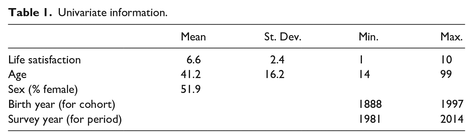
Univariate information.

	Mean	St. Dev.	Min.	Max.
Life satisfaction	6.6	2.4	1	10
Age	41.2	16.2	14	99
Sex (% female)	51.9
Birth year (for cohort)			1888	1997
Survey year (for period)			1981	2014

In brief, the reason to avoid individual-level controls such as income, marital status and education is that these aspects of people’s lives cannot determine one’s age. In the first instance, the reason to include control variables in a regression model is to mitigate against the possibility of bias – confounding bias, in particular (e.g. Shahar and Shahar, 2013). Confounding bias emerges from the omission of variables that determine the dependent variable and also the core independent variable of interest. Income, marital status and education all help determine life satisfaction – but again they do not (and indeed cannot) determine how old one is. Instead, they are intervening variables: getting older typically has impacts on, for example, one’s income and one’s marital status – impacts that then affect life satisfaction. They are not ‘confounders’ and (at least initially) should therefore not be included in regression models seeking to gauge the effect of age. The only necessary control variables are cohort, period and (for multi-country studies) country; these can determine age (i.e. the age composition of the population) as well as life satisfaction and are therefore potential confounders.

This article offers researchers greater clarity on these points by reinforcing important distinctions: between confounding and intervening variables, and between total effects, direct effects and indirect effects. To gauge ‘the effect’ of age, one starts with a regression model that includes confounders (if any) but excludes intervening variables. Having thus identified a total effect, one could then attempt to understand it further by considering the role of intervening variables: adding controls for intervening variables enables identification of indirect effects (e.g. the effect of age that runs through age’s impact on income and income’s subsequent impact on life satisfaction). With controls for intervening variables, any remaining effect of age might be described as the direct effect of age (though one could likely push further in this respect by seeking additional intervening variables).

Many researchers investigating life satisfaction (as well as happiness) do not write about the important distinction between confounding variables and intervening variables. One therefore sees many regression models (in this field and many others) that are not properly specified, in the sense that they do not give results that identify ‘the effect’ (i.e. the total effect) of particular variables, because they include intervening variables. There is an obvious need for greater clarity in this regard, in particular to avoid what is sometimes called ‘overcontrol bias’ (e.g. Elwert and Winship, 2014).

The article proceeds in the next section with a discussion of the logic of control variables in regression models. This discussion comes in lieu of a (further) review of previous findings about age and life satisfaction. The dispute is effectively summarized above,² and the issue in contention is methodological, not substantive. (That is, the differences in findings are not rooted in disagreement about why one might expect age to affect life satisfaction in particular ways, e.g. from different theoretical positions.) What is needed is a better understanding of what regression models do, depending on what types of control variables are included. I first develop the core point about intervening vs. confounding variables via a simple example. I proceed to describe the limitations evident in researchers’ interpretations of regression models containing intervening controls, with particular attention to the distinction between direct and indirect effects. The article then presents an analysis of data from rounds 1–6 of the World Values Survey (WVS), with models specified to exclude intervening variables. It concludes by emphasizing the importance (in quantitative research) of giving much more thorough attention to the question of what variables to include as controls in one’s models – a point with wide applicability, well beyond the topic of age and life satisfaction.

Confounding vs. Intervening Variables

Commonly used statistics/econometrics textbooks teach students to deploy control variables without making an important distinction – between confounders and intervening variables (e.g. Hair et al., 2013; Wooldridge, 2015). Regression is conventionally treated as a fundamentally mathematical exercise, with ‘prediction’ as the core goal. While there is often a nod to ‘theory’ as a basis for selecting additional independent variables, the main criterion is mathematical: does adding a variable improve ‘model fit’? It is then unsurprising to encounter confusion and misspecification in empirical work. This tendency is likely reinforced by an implicit belief that models are ‘better’ (or perhaps at least more impressive) when they contain more control variables.

Two simple examples illustrate why a different approach is needed for gaining insight into how the social world works. An example sometimes used for teaching involves height and maths ability. Even without a regression model, one could see via a scatterplot that there is a positive relationship: taller people are better at maths. An empirical description along these lines would be entirely correct; a (bivariate) regression model would only provide additional detail, for example a coefficient for the slope. As odd as it might seem, height is a useful ‘predictor’ of maths ability – a point that shows the limitations of findings expressed via the language of prediction.

As the saying goes: correlation is not causation. We can reasonably ask: are taller people better at maths because they are taller? We might suspect that there is some other factor that determines both height and maths ability. Such a factor is not difficult to find: among children, age makes people taller, and it also leads to an improvement in their maths ability. If we control for age, height has no correlation at all with maths ability. Age is a confounder here, and if we omit it from our analysis, we get substantial bias in our (initial) result (suggesting an impact of height on maths ability). Researchers sometimes use the notion of ‘spuriousness’ to describe this pattern: the apparent relationship between height and maths ability is obviously spurious. But ‘confounding bias’ is useful as a more general category: some correlations involve so much confounding bias that the apparent relationship is (entirely) spurious – but in other cases there is simply some bias in one’s coefficients, without the relationship being altogether spurious. Including the right control variables (i.e. the ones that are determinants of the main independent variable) reduces bias.

But some potential controls are not determinants of the main independent variable – instead, they are determined by the main independent variable. In other words, they intervene in a path from the main independent variable to the outcome variable. Including these variables as controls in one’s model will exacerbate bias rather than reducing it. For example, if we wanted to estimate the effect of unemployment on life satisfaction, it would be an error to include a control for income – because income is determined by unemployment (getting sacked typically results in a substantial reduction of income). If we control for income, the coefficient for unemployment now gives us the impact of unemployment on life satisfaction for people at the same level of income. Including this control obscures part of the impact of unemployment on life satisfaction: it gives us an estimate for unemployment’s effect that does not reflect the way unemployment lowers income and the reduction of income itself reduces life satisfaction. Inclusion of that variable ‘controls away’ this component of unemployment’s effect. So, the estimate is now biased, as an indication of the total effect of unemployment on life satisfaction; specifically, a model that includes income will understate the effect of unemployment on life satisfaction, giving a figure that is too low (relative to the actual effect).

In general, then: regression models designed to gauge the effect of a particular variable should include confounding variables and exclude intervening variables (e.g. Berk, 1983; Gangl, 2010; Pearl, 2018; Smith, 1990). The purpose of control variables is to minimize bias in one’s estimates – but this purpose is achieved only if the controls we add are confounders; that is, variables that are causally prior to the independent variable whose impact we seek to identify. Adding control variables does not have a single/unitary impact on the results given by our models. To understand their impact, we must consider this distinction between confounders and intervening variables.

A necessary caveat is that for some variables the situation is less clear than a binary opposition between confounding and intervening variables might imply. Some variables might belong to both categories. In situations of that sort, one must make a judgement as to which type of effect is likely to dominate (i.e. the strength of the two effects), given the substantive question one seeks to answer. If the intervening path dominates the confounding path, one likely loses more than one gains by including the variable as a control; including it is likely to exacerbate bias rather than to reduce it. The matter should be discussed in substantive terms, perhaps as a limitation of one’s analysis.

Reconsidering the Relationship between Age and Life Satisfaction

The points in the preceding section offer increased clarity on what sort of analytical approach to use for investigating the relationship between age and life satisfaction. An analysis that mostly excludes individual-level controls is required. Such an analysis is not biased via omission of other variables – because most other variables cannot be confounders in this context. Other variables help determine life satisfaction, but they do not affect age. Again, they cannot do so; certain variables might affect the age composition of a population, but they cannot determine the age of any particular individual.

Researchers who produce results relying on regression models that contain individual-level controls sometimes describe the age coefficient(s) as the ‘net’ or ‘pure’ effect of age (Blanchflower and Oswald, 2019). Interpretations of that sort are formally correct – but they can be understood properly only via precise articulation regarding what the ‘net effect’ is net of. A useful language for this idea is that they are ‘direct’ effects, net of the indirect effects that run through paths containing intervening variables. When one includes intervening variables, it is misleading to state that the coefficient for age is ‘net of the effects of other variables’; the other variables are determined in part by age, and when one controls for those other variables the results for age are net of the indirect effects of age itself.

So, if income, for example, is to be included as a control, we then need to understand how age would affect income, and how the resulting changes in income would affect life satisfaction. Assume a positive impact of income on life satisfaction, and assume as well that income rises towards middle age (or perhaps towards retirement age) and then declines after retirement (a pattern that reasonably describes the experience of many) – in other words, an inverse-U. If we control for income in a model investigating age, the results for the age coefficient will be altered by control of the path on which age (indirectly) increases life satisfaction towards middle age via its (age’s) earlier positive effect on income. We also mitigate the way age would (indirectly) decrease life satisfaction after retirement via its (age’s) later negative effect on income. If age in general had no particular impact on life satisfaction (i.e. if it was basically flat as per Diener et al.’s (1999) early position), controlling for income might foster the impression of a U-shape: in the circumstances described here, controlling for income will reduce the coefficient for age and raise the coefficient for age-squared. But this impression would be misleading in regard to ‘the effect’ of age.

The idea of a net/direct effect is sensible on its own terms; we might well be interested in some notion of a ‘pure’ impact of age, distinct from its impact via income (or indeed other circumstances). That impact might be articulated with reference to the way age itself can make people feel: being old might make one feel depressed and useless (especially in a society valuing youth) – or, in contrast, it might lead to a sense of peace rooted in ‘wisdom’ or acquiescence (notions that are not directly connected to income or other aspects of one’s circumstances). But a sensible interpretation along these lines requires explicit articulation – at a minimum, so that readers (and especially journalists) are not led to believe that they are being presented with the total effect of age. ‘The effect’ of age is the total effect: in addition to direct effects, ageing changes people’s circumstances, and the changes in their circumstances affect how satisfied they are with their lives.

The situation is quite complicated in any scenario where more than one intervening control variable is included. When regression models contain multiple controls, we must think of coefficients for particular variables in ceteris paribus terms – the effect of one variable holding all the other variables constant. So, if age affects income and income affects some other variable (say, health) that has its own effect on life satisfaction, understanding the indirect paths becomes a challenging endeavour. Using regression models to analyse individuals’ experiences is a risky enterprise unless great care is taken to consider the logic of including particular control variables; the controls likely have relationships not just with the core independent variable and the dependent variable but with one another as well. Those relationships will be important in one’s understanding of what the indirect effects of age are – a point that then affects our understanding of what constitutes the direct effect.

If a model is specified to control only for confounders pertaining to the core independent variable of interest, then considerations of this sort do not arise; the model will give the total effect for that variable. If the goal is to investigate ‘the effect’ (e.g. of age), then a properly specified model is one that includes controls for variables understood to be confounders (and excludes variables understood to be intervening). For age, there are no individual-level confounding variables to control for; the only appropriate controls are cohort, period and country (and possibly sex), as discussed below. Other variables might be important determinants of life satisfaction, but the ‘usual suspects’ cannot be determinants of age.

Data and Analytical Approach

With these considerations in mind, we turn to an empirical investigation of how (or indeed whether) age affects life satisfaction. Data are taken from Waves 1 through 6 (survey periods: 1981/1984 to 2010/2014) of the WVS (Inglehart et al., 2014). Countries that participated only once are not suitable for effective treatment of cohort and so are dropped from the analysis; we then have 69 countries representing a wide variety of (country-level) situations.³ National samples are constructed to be representative of the population; interview mode is face-to-face at the respondent’s home. Total sample size is 304,131; the per-round average across the countries included here is 1505. The sample as analysed below is N = 298,547; cases are dropped where needed variables are missing – an issue that arises mostly at the level of country-rounds (not individuals). The low number of dropped cases together with a consideration of the main mechanism for this type of missing data is a reasonable indication that missing data do not distort the findings reported below.

Life satisfaction is given in answer to the question, ‘All things considered, how satisfied are you with your life as a whole these days?’ Respondents choose a number from 1 to 10, where 1 is ‘completely dissatisfied’ and 10 is ‘completely satisfied’ (with the intervening numbers unlabelled). Age is derived from a question about the respondent’s year of birth; respondents are also asked to confirm their age.

The relevant controls in this context are cohort, period and country, each of which can influence population age composition as well as life satisfaction. The effect of country on age composition is evident via the significant international variation in life expectancy. To correctly perceive the general relationship between age and life satisfaction, one must adjust for the age-composition effect of mortality: if there are contextual factors that increase early mortality and also tend to reduce life satisfaction, the absence (from the sample) of older respondents affected by those patterns will artificially raise the coefficient of an age variable describing the experience of older people. The same possibility pertains to cohort and period effects. One can also include sex for this purpose: it too can affect the age composition of a population and might help determine life satisfaction. Crucially, it is ‘safe’ as a control variable because it cannot be an intervening variable (age cannot determine one’s sex).

Following Yang (2008), cohort is constructed in five-year spans working backwards from the year of birth of the youngest respondent in the Wave 6 sample. The use of five-year spans for the cohort variable allows analysts to ‘break’ the linear dependency that otherwise impairs age–period–cohort analysis (without making arbitrary assumptions about time trends). The variable for period is simply the year in which the respondent participated in the survey.

The analysis presents results from cross-classified random-effects models (CCREM), developed by Yang (2008) and Yang and Land (2008) for investigation of age effects using repeated cross-sectional datasets (as with the WVS here). ‘Random effects’ address the clustering associated with the (Level 2) country, cohort and period variables, using a multi-level modelling framework; this approach is preferable to entering these variables as fixed effects in a way that ignores the clustering. The higher-level variables are not fully nested within one another; the ‘cross-classification’ angle allows in particular for the possibility that people in the same birth cohort might be interviewed in different periods (and vice versa). Within this framework, age and sex are entered as fixed effects at Level 1; in this respect the model yields coefficients for those variables that are equivalent to the results given by ordinary least-squares models.⁴

The conventional approach for this question is to construct models containing a quadratic function for age; that is, age-squared as well as age. But this approach produces coefficients that are difficult to interpret.⁵ If both terms are statistically significant, one is led to conclude that there is indeed a U-shape, but it is difficult to determine how much life satisfaction falls and then rises (and when the increase begins). An evaluation of effect size, not just statistical significance, is needed. To consider effect size, I adopt a more straightforward approach. The idea of U-shape again suggests that life satisfaction declines with age through middle age and subsequently rises. To evaluate that proposition directly, it is more profitable to split the sample (so, investigating younger and older people separately) and abandon the age-squared term (cf. Piper, 2015). The analysis below uses a cut-off of 45 for this purpose; this figure was chosen via exploration of other possibilities where it became apparent that a cut-off of 45 maximized the magnitude of the subsequent rise in life satisfaction to the age of 85 (the other cut-offs produced a smaller value). The analysis also considers results from a more conventional model with a quadratic age function. All models include weights so that the influence of respondents from different countries is proportional to the relative population/size of the country (within the 69 countries investigated here).

Some researchers (e.g. Cheng et al., 2017; Jivraj et al., 2014; Kassenboehmer and Haisken-DeNew, 2012) turn to panel data, believing that a longitudinal analysis is superior to inferring change from cross-sectional comparison of older to younger people. If there were panel data that covered people’s entire adult lives, it would indeed be very useful for the purpose of understanding how life satisfaction changes across the life course. But existing panels are much shorter; to understand what will happen to younger people as they become much older, it is still necessary to extrapolate from the ‘current’ experience of much older people (and vice versa), in a manner equivalent to cross-sectional analysis (cf. Frijters and Beatton, 2014). Another reason to use panel data is to enable application of fixed-effects techniques that control for unmeasured time-invariant characteristics. If there were grounds for concern about the existence of unmeasured characteristics that amounted to potential confounders in this context, then one could make a good case that a fixed-effects analysis is superior. But we return to a core premise of this article: other individual-level factors (even the unmeasured ones) cannot be confounders in this context, because they cannot determine one’s age. From that angle, a cross-sectional analysis (comparison of older to younger people at one point in time) gives a good indication of how becoming older will (or will not) affect people’s life satisfaction.⁶ A fixed-effects analysis is by no means inappropriate or defective (though it should not include individual-level control variables) – but one would not opt for it over a cross-sectional regression analysis on grounds of worry about unmeasured confounders.

A third potential advantage of longitudinal methods is that they enable consideration of ‘reverse causation’: perhaps people live longer when they are more satisfied with their lives, and if we do not account for the way this process leads to lower representation of older less-satisfied people in the sample, a cross-sectional analysis gives a biased result for the effect of age on life satisfaction (the main relationship under consideration) via sample composition. Importantly, the direction of that bias would be upwards especially for older people: if the sample contained people whose death had been caused in part by poor life satisfaction, the result describing the overall effect of ageing would be lower than it appears in a conventional cross-sectional analysis based on living respondents. We then face a trade-off: a cross-sectional approach might give results that are biased in the way we have just described, but on the other hand we can consider a much wider range of countries, so that our impressions are not determined solely by countries where panel data are available. Given this trade-off, a cross-sectional analysis is worth pursuing, and the possibility of bias can be considered a potential limitation (and will be discussed further in connection with results below).

Table 1 offers univariate information on the variables included in the analysis.

Results

Table 2 first reports results from separate models for older and younger respondents. The left portion of the table (Model 1) indicates that life satisfaction indeed declines across the younger age range – at an average rate of 0.0082 points per year on the 10-point scale. This is not a greatly ‘significant’ number in a substantive sense, though it is perhaps a genuine decrease. (After 10 years, a younger person’s life satisfaction will have declined by almost one-tenth of a point on the 10-point scale, on average.)

Table 2.

Cross-classified random-effects models of life satisfaction.

	Model 1: under 45		Model 2: 45 and older		Model 3: all respondents
	b	s.e.	b	s.e.	b	s.e.
Age	−0.0082	0.0017***	0.0025	0.0012*	−0.0015	0.0023
Age-squared					−0.0000	0.0000
Female	0.0859	0.0105***	−0.0951	0.0135***	0.0189	0.0083
Constant	6.8331	0.1400***	6.5228	0.1649***	6.7616	0.1517
Random effects – variance components:
σ² Cohort	0.009		0.004		0.022
σ² Survey year (period)	0.144		0.128		0.127
σ² Country	0.659		1.085		0.830
σ² Residual	5.206		4.969		5.128
Log likelihood	−491,496		−313,140		−804,911
N	183,485		115,062		298,547

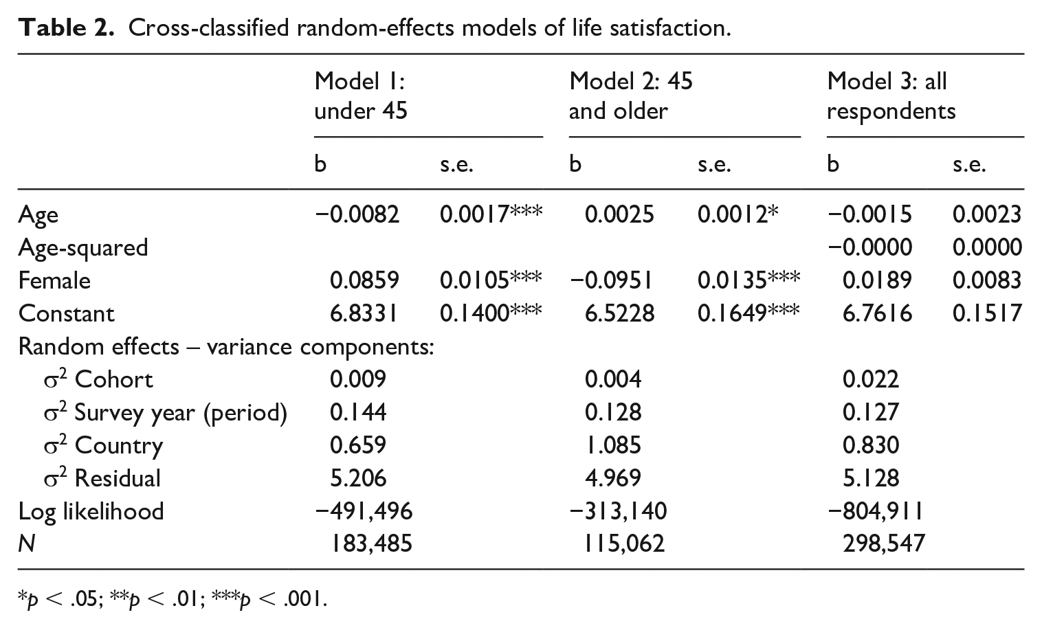
p < .05; **p < .01; ***p < .001.

But Model 2 fails to provide support for the notion that life satisfaction rises ‘significantly’ after the cut-off age of 45. The coefficient is positive but tiny: 0.0025, less than one-third of the pre-middle-age decline. It is statistically significant (at p < .05) – but virtually any variable could be statistically significant with a sample size of more than 115,000.⁷ One could probably succeed in publishing an article concluding on this basis that there is a ‘significant’ increase in life satisfaction after 45 – but this is not a sensible conclusion given the effect size. We are now in a position to conclude that any post-middle-age increase in life satisfaction is in fact negligible: starting at age 45 and moving forward to the age of 85, the average total increase in life satisfaction would be one-tenth of a point on the 10-point scale. A conventional measure of effect size (Cohen’s D) for this increase over 40 years gives d = 0.04 (the standard deviation of the life satisfaction variable for people 45 and older is 2.5, so: 0.0025 * 40 / 2.5 = 0.04) – a very small figure, certainly in comparison to the rule of thumb where ‘small’ = 0.2.

This latter finding is a significant blow against the idea of ‘U-shape’. It is robust to the choice of cut-off; for no value do we get a result suggesting any more substantial rise in life satisfaction after middle age (the additional values explored were 50, 55, 60 and 65; results available on request). Without some substantial increase after middle age, there can be no U-shape.

The results from Model 3 of Table 2 reinforce this conclusion: here as well there is no indication of an upturn in post-middle-age life satisfaction. In a conventional model containing a quadratic function for age, the coefficient of the age-squared term is negative (as is the coefficient for raw age), though also tiny at −0.00002 and not statistically significant.

Figure 1 offers a visual representation of the conclusions we derive from the linear analyses here (Models 1 and 2): the lines indicate a mostly ‘flat’ trend in life satisfaction especially among older respondents. A visual representation of the results from Model 3 would consist of a flat line, at least in the sense that the age coefficients from that model are not statistically significant.

Figure 1.

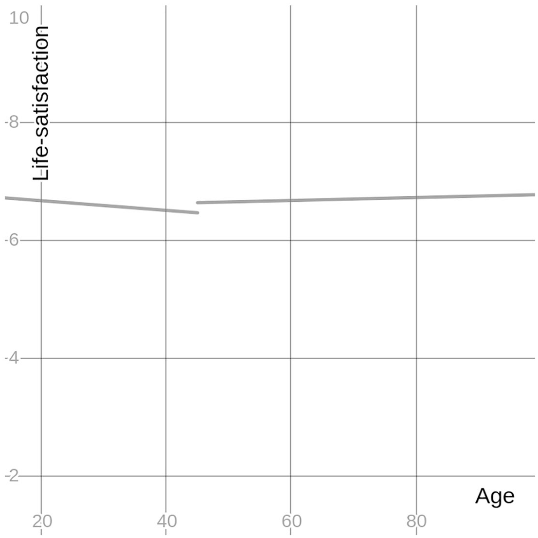
Age and life satisfaction.

The WVS sample across the six rounds contains a wide range of countries, and we should expect to find diversity in findings across that range (Deaton, 2008; Steptoe et al., 2015). Table 3 replicates the analysis described above (with cut-off at 45)⁸ for each of the 69 countries (a random-effect term for country is now excluded). The table (containing only the coefficients for age) indeed reveals a diverse set of patterns. For some countries we see results that support the conclusion of U-shape: life satisfaction generally falls and then rises in the Czech Republic, Mexico and Turkey. That conclusion uses a threshold of p = .05 for statistical significance; in each case the post-middle-age increase is similar in magnitude to the pre-middle-age decrease.⁹ But the pattern is quite different for other countries. In Australia one sees an increase in life satisfaction across the adult life course; for some countries there is an increase after age 45 but no pre-45 decline (Algeria, Netherlands, New Zealand, Singapore, South Africa, Sweden, Switzerland, UK, USA, Uruguay). A continuous decline across the adult life course is evident for Bulgaria, Georgia, Moldova, Pakistan, Romania, Serbia, Slovenia, Spain and Ukraine (it is likely no coincidence that seven of those are post-communist countries). Even at the level of countries, then, we do not discern a U-shape in the sense that for a broad range of countries life satisfaction falls and then rises; most countries analysed here do not show that pattern. One could ask how to explain why different patterns are apparent in different countries – but this question is left for future research. The relevant point here is simply that the U-shape pattern is not evident for most of the countries covered by WVS data.

Table 3.

Age and life satisfaction by country and age group (CCREM regressions, controlling for sex, cohort and period).

	Under 45	45 and older		Under 45	45 and older
	b	b		b	b
Albania	−0.009	−0.033**	Montenegro	−0.004	−0.024*
Algeria	−0.017	0.027*	Morocco	0.006	0.014
Argentina	−0.014**	0.004	Netherlands	0.000	0.012***
Armenia	−0.054***	−0.003	New Zealand	0.000	0.025***
Australia	0.011**	0.020***	Nigeria	−0.020***	−0.006
Azerbaijan	−0.015+	−0.008	Norway	0.000	0.002
Bangladesh	−0.026+	−0.009	Pakistan	−0.026***	−0.029**
Belarus	−0.034***	−0.002	Peru	−0.016***	0.010
Brazil	0.005	0.011	Philippines	−0.020*	0.006
Bulgaria	−0.028**	−0.021**	Poland	−0.030***	0.001
Canada	−0.008	0.005	Puerto Rico	−0.005	0.010
Chile	0.005	0.000	Romania	−0.041***	−0.011+
China	−0.007	0.020***	Russia	−0.045***	−0.005
Colombia	0.002	−0.002	Rwanda	−0.016*	−0.011
Cyprus	−0.012	0.009	Serbia	−0.026***	−0.019**
Czech Rep.	−0.031**	0.017*	Singapore	0.006	0.013*
Egypt	−0.010	0.010	Slovakia	−0.034***	0.002
Estonia	−0.048***	−0.002	Slovenia	−0.035***	−0.021***
Finland	−0.013+	0.004	South Africa	−0.004	0.017***
Georgia	−0.040***	−0.016**	South Korea	0.009+	−0.014*
Germany	−0.008	0.002	Spain	−0.007+	−0.006+
Ghana	−0.028***	−0.009	Sweden	0.006	0.015***
Hong Kong	0.009	−0.007	Switzerland	−0.008	0.014***
Hungary	−0.045***	0.011	Taiwan	−0.004	−0.012+
India	−0.004	−0.012**	Thailand	−0.010	−0.008
Indonesia	0.004	−0.011	Trinidad and Tobago	−0.006	0.011
Iran	−0.005	−0.007	Turkey	−0.015***	0.015*
Iraq	−0.017**	0.004	Ukraine	−0.045***	−0.030***
Japan	−0.007+	0.023***	United Kingdom	0.006	0.024***
Jordan	−0.002	0.015+	United States	−0.005	0.013***
Kyrgyzstan	−0.028***	−0.015	Uruguay	−0.009	0.014**
Macedonia	−0.018+	0.016+	Venezuela	−0.009	0.010
Malaysia	0.014*	−0.014	Vietnam	0.007	−0.005
Mexico	−0.011**	0.010*	Zimbabwe	−0.048***	−0.005
Moldova	−0.034***	−0.018**

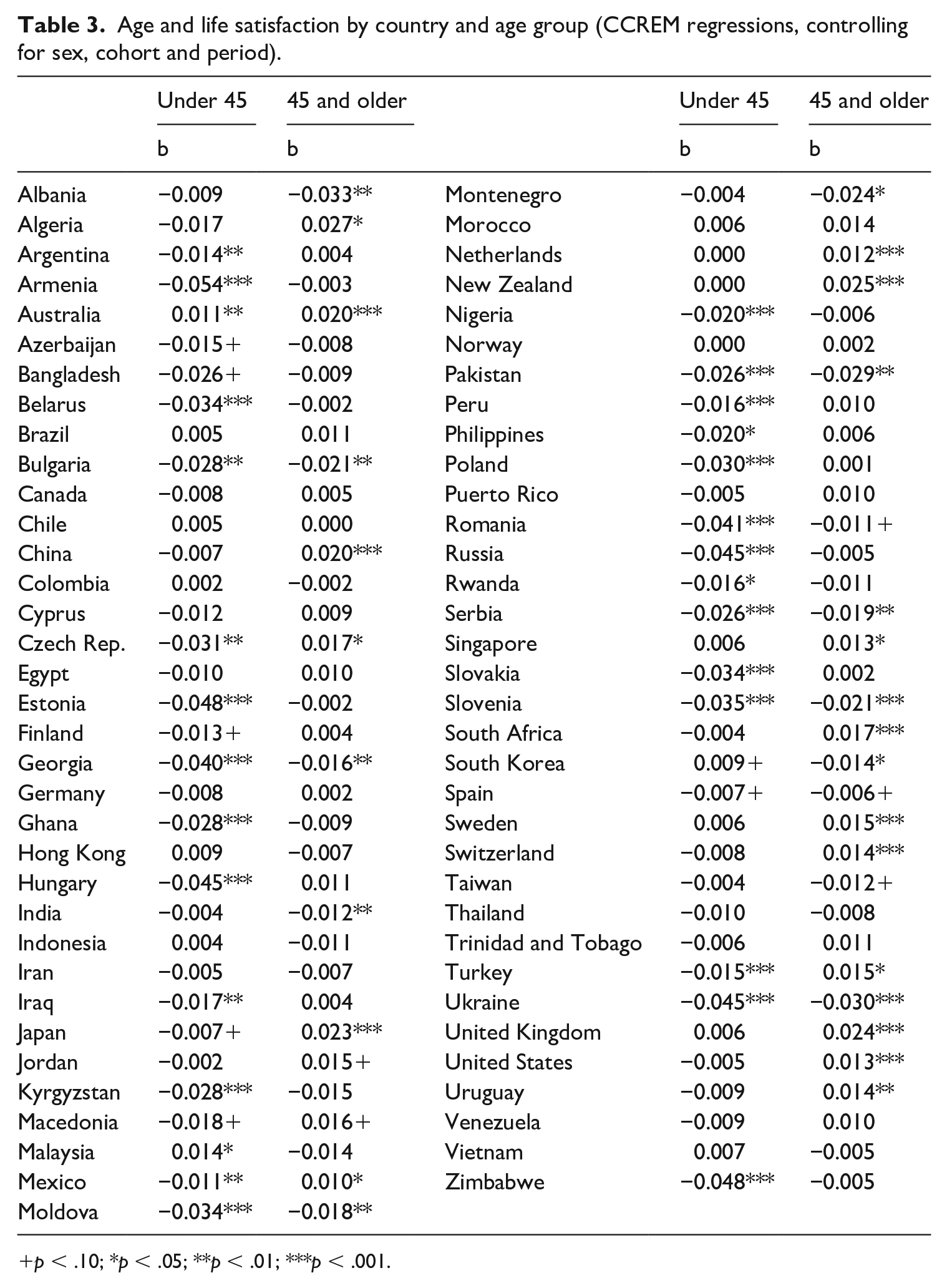
p < .10; *p < .05; **p < .01; ***p < .001.

What remains is to consider the possibility that some potential individual-level control variables might in this context be confounding as well as intervening. The possibility of a confounding effect exists only at the level of sample composition; individual-level variables cannot determine how old a person is, they can only affect sample composition by affecting the likelihood of early mortality. An obvious candidate is health: to state the obvious, people in poor health (especially older people in poor health) are at greater risk of dying. To mitigate against bias emerging from that possibility, one could consider including health as a control. But the costs of doing this surely outweigh any benefits. Any confounding bias arising from the omission of health is likely to be dwarfed by the bias induced by including it, given the way health intervenes in the relationship between age and life satisfaction. Age generally leads to poorer health; poorer health leads to lower life satisfaction. If we control for health, we will get an artificially raised coefficient for the effect of age. That coefficient is now a direct effect, net of the (negative) indirect effect of age that travels via its effect on health. If we interpreted it as the total effect, we would be presenting a figure that we have good reason to think is substantially biased. In contrast, the confounding bias associated with omitting health is by definition marginal; it does not pertain to the experience of people still alive (who are thereby available to participate in surveys). Including it is likely to exacerbate bias, not reduce it.

Empirical results verify intuitions about the consequences of including health. In models equivalent to those in Table 1 (adding a five-category variable for subjective health: very poor; poor; fair; good; very good), the age coefficient for those under 45 is now less negative (–0.0020 instead of −0.0082), and for those over 44 the age coefficient is more positive (0.0109 instead of 0.0025). Adding health has raised the age coefficients – but it has not given us a better understanding of the way age affects life satisfaction, expressed as a total effect (so, a table is not included here). Instead, it has obscured the way age often leads to worse health, which then depresses life satisfaction; the age coefficients are artificially high as a consequence of excluding that indirect effect.

One could consider other variables (e.g. education, income, partner) in similar terms. In each case, the fact that any confounding effect would operate only via sample composition means that inclusion would predictably induce bias via intervening effects.

We note again the potential implication of bias in cross-sectional results, emerging from the possibility of reverse causation: people with lower life satisfaction might experience poorer health (Steptoe et al., 2015), which might lead to early mortality. We can do more than simply accept a generic limitation for our cross-sectional results in connection with this possibility (‘the results might be biased’): we can consider the likely direction of bias. As argued above, the bias is likely positive – so, unbiased results for the impact of age on life satisfaction are likely to be lower than what is reported above, especially for older people. If low life satisfaction increases the odds of mortality, we will lack data on some people who have low life satisfaction especially in old age. The absence of such people from our sample means the coefficient describing the age impact on older people is higher than it would otherwise be. The main substantive result of this article is that there is no substantial increase in life satisfaction after middle age (and thus no U-shape) – and the possibility of reverse causation does not undermine that conclusion (and in fact would tend to reinforce it).

Conclusion and Implications

In a key contribution to this debate, Blanchflower and Oswald (2008) ask (in their title): ‘is well-being U-shaped over the life cycle?’ At least for the countries analysed here, that question has a straightforward answer: no. That answer applies to these countries taken as a whole and individually to 66 of the 69. One might be tempted to draw on the statistically significant age coefficient for the regression model pertaining to older respondents. But a responsible reporting of that finding should contain the following caveat: if there is a U-shape, the actual change in life satisfaction associated with age is very small, with only a negligible upturn in later life.

This answer is rooted in the assertion that the right answer comes from models without individual-level controls apart from sex (so, including controls mainly for the higher-level variables of country, cohort and period). Blanchflower and Oswald (2019) offer a rebuttal that might seem appealing: neither approach is incorrect – each gives different information.¹⁰ That position is appealing only on the surface; it holds up in regard to the ‘control for other determinants’ position only if the results from that approach are interpreted correctly – that is, as the direct effect of age when the indirect effects of age have been controlled away. Again, that interpretation is correct, but results are usually not articulated with that sort of precision.¹¹

Should researchers continue the common practice of including age as a control variable in models intended for other purposes? Yes. Even if there is no general U-shape, age affects people’s life satisfaction in a large number of countries. It also affects other aspects of their situations (e.g. income, health, marital status, etc.). It is therefore a plausible confounder in most situations – and it cannot be an intervening variable.

Whether it makes sense to include an age-squared term is another matter. If one can make a sensible case for why a quadratic function is relevant to the process under consideration, then perhaps – but doing this runs the risk of reinforcing the mistaken impression that age and life satisfaction have a U-shaped relationship. A statement of that sort, even if accompanied by a ‘ceteris paribus’ condition, might mislead readers, especially given the extent of misunderstanding about this relationship resulting from prior research. Proper interpretation of results for control variables requires care; if models were specified correctly to gauge the effect of the core independent variable of interest, then they are probably not specified for results regarding the (total) effects of control variables. To be technically correct, one can always simply invoke the ‘ceteris paribus’ clause – but again that clause might obscure a great deal.

What is genuinely needed is a more detailed and substantive justification for selection of control variables in one’s model. Many researchers provide virtually no justification at all: one commonly sees (certainly in research on happiness/life satisfaction) a notion of a ‘standard set’ of controls. At a minimum, researchers need to use the core distinction emphasized here, between confounding and intervening variables. Heeding this distinction could be consequential especially for research exploring the effects of characteristics that for most people are very unlikely to change (e.g. sex and ‘race’), and for questions pertaining to the impact of experiences earlier in life, where control variables might create indirect effects on paths leading to the dependent variable.

Even if there is no apparent upturn in life satisfaction after middle age, it is perhaps remarkable that life satisfaction does not generally decline as people become old. Of course, in some countries there is a decline; when ageing is associated with poverty, for example in the absence of a welfare state, life in old age can become difficult (though in most of the wealthier societies a welfare state can help counteract this trend). Even so, given the other challenges ageing can bring – poor health and loss of partner, in particular – one might expect a decline in life satisfaction to be quite common. The fact that the overall trend is flat might point to a genuine direct effect of age: as many proponents of ‘U-shape’ suggest (e.g. Schwandt, 2016), ageing might bring mitigation of unrealistic aspirations, a focus on the present, stoicism and so on. But that direct effect does not seem to bring about an actual increase in life satisfaction; it appears merely to counteract what would otherwise be a decline in life satisfaction rooted in the genuine challenges of growing old.

Footnotes

Acknowledgements

I am very grateful for feedback on earlier drafts from Martijn Hendriks, Patrick White and Jing Shen. Early versions of the article were presented to the Mannheim Centre for European Social Research (March 2019) and to the Wittgenstein Centre Conference 2019 on ‘Demographic Aspects of Human Wellbeing’.

Funding

The author received no financial support for the research, authorship and/or publication of this article.

ORCID iD

David Bartram

Notes

David Bartram is Associate Professor in Sociology at the University of Leicester. His research focuses on subjective well-being and international migration – for example, investigating the idea that migration to a wealthy country is advantageous to the migrants themselves. He has held a grant (with colleagues at Leicester) from the UK Economic and Social Research Council, as well as awards from Leverhulme and the Nuffield Foundation. He has published two books: Key Concepts in Migration (SAGE, with Maritsa Poros and Pierre Monforte) and International Labor Migration: Foreign Workers and Public Policy (Palgrave). He is co-editor of the Journal of Happiness Studies and President of RC31, the section on the Sociology of Migration of the International Sociological Association. He holds a PhD from the University of Wisconsin–Madison and a BA from Kenyon College.

References

Beja

(2018) The U-shaped relationship between happiness and age. Quality & Quantity 52(4): 1817–1829.

Berk

(1983) Regression Analysis: A Constructive Critique. Los Angeles, CA: SAGE.

Blanchflower

Oswald

(2004) Well-being over time in Britain and the USA. Journal of Public Economics 88(7–8): 1359–1386.

Blanchflower

Oswald

(2008) Is well-being U-shaped over the life cycle? Social Science & Medicine 66: 1733–1749.

Blanchflower

Oswald

(2009) The U-shape without controls: A response to Glenn. Social Science & Medicine 69(4): 486–488.

Blanchflower

Oswald

(2019) Do humans suffer a psychological low in midlife? Two approaches (with and without controls) in seven data sets. In: Rojas

(ed.) The Economics of Happiness. Cham: Springer International Publishing, 439–453.

Cheng

Powdthavee

Oswald

(2017) Longitudinal evidence for a midlife nadir in human well-being. The Economic Journal 127(599): 126–142.

Deaton

(2008) Income, health, and well-being around the world: Evidence from the Gallup World Poll. Journal of Economic Perspectives 22: 53–72.

Diener

Suh

Lucas

, et al. (1999) Subjective well-being: Three decades of progress. Psychological Bulletin 125: 276–303.

10.

Easterlin

(2006) Life cycle happiness and its sources: Intersections of psychology, economics, and demography. Journal of Economic Psychology 27: 463–482.

11.

Elwert

Winship

(2014) Endogenous selection bias: The problem of conditioning on a collider variable. Annual Review of Sociology 40(1): 31–53.

12.

Frijters

Beatton

(2014) The mystery of the U-shaped relationship between happiness and age. Journal of Economic Behavior & Organization 82(2–3): 525–542.

13.

Gangl

(2010) Causal inference in sociological research. Annual Review of Sociology 36(1): 21–47.

14.

Glenn

(2009) Is the apparent U-shape of well-being over the life course a result of inappropriate use of control variables? A commentary on Blanchflower and Oswald. Social Science & Medicine 69(4): 481–485.

15.

Gorard

(2016) Damaging real lives through obstinacy: Re-emphasising why significance testing is wrong. Sociological Research Online 21(1): 1–14.

16.

Graham

Ruiz Pozuelo

(2017) Happiness, stress, and age: How the U curve varies across people and places. Journal of Population Economics 30(1): 225–264.

17.

Hair

Black

Babin

, et al. (2013) Multivariate Data Analysis. London: Pearson Education UK.

18.

Hellevik

(2017) The U-shaped age–happiness relationship: Real or methodological artifact? Quality & Quantity 51(1): 177–197.

19.

Inglehart

Haerpfer

Moreno

, et al. (2014) World Values Survey: Round Six. Madrid: JD Systems Institute. Available at: www.Worldvaluessurvey.Org/WVSDocumentationWV6.Jsp.

20.

Jivraj

Nazroo

Vanhoutte

, et al. (2014) Aging and subjective well-being in later life. The Journals of Gerontology Series B: Psychological Sciences and Social Sciences 69(6): 930–941.

21.

Kassenboehmer

Haisken-DeNew

(2012) Heresy or enlightenment? The well-being age U-shape effect is flat. Economics Letters 117(1): 235–238.

22.

Laaksonen

(2018) A research note: Happiness by age is more complex than U-shaped. Journal of Happiness Studies 19(2): 471–482.

23.

López Ulloa

Møller

Sousa-Poza

(2013) How does subjective well-being evolve with age? Journal of Population Ageing 6(3): 227–246.

24.

Pearl

(2018) The Book of Why: The New Science of Cause and Effect. London: Allen Lane.

25.

Piper

(2015) Sliding down the U-shape? A dynamic panel investigation of the age–well-being relationship, focusing on young adults. Social Science & Medicine 143: 54–61.

26.

Rauch

(2018) The Happiness Curve: Why Life Gets Better after Midlife. London: Bloomsbury Publishing.

27.

Schwandt

(2016) Unmet aspirations as an explanation for the age U-shape in wellbeing. Journal of Economic Behavior & Organization 122: 75–87.

28.

Shahar

(2013) Causal diagrams and the cross-sectional study. Clinical Epidemiology 5: 57–65.

29.

Simonsohn

(2018) Two lines: A valid alternative to the invalid testing of U-shaped relationships with quadratic regressions. Advances in Methods and Practices in Psychological Science 1(4): 538–555.

30.

Smith

(1990) Specification problems in experimental and nonexperimental social research. Sociological Methodology 20: 59–91.

31.

Steptoe

Deaton

Stone

(2015) Subjective wellbeing, health, and ageing. The Lancet 385(9968): 640–648.

32.

Wooldridge

(2015) Introductory Econometrics. Mason, OH: Cengage Learning.

33.

Yang

(2008) Social inequalities in happiness in the United States, 1972 to 2004: An age–period–cohort analysis. American Sociological Review 73(2): 204–226.

34.

Yang

Land

(2008) Age–period–cohort analysis of repeated cross-section surveys: Fixed or random effects? Sociological Methods & Research 36(3): 297–326.

Age and Life Satisfaction: Getting Control Variables under Control

Abstract

Keywords

Introduction

Confounding vs. Intervening Variables

Reconsidering the Relationship between Age and Life Satisfaction

Data and Analytical Approach

Results

Conclusion and Implications

Footnotes

Acknowledgements

Funding

ORCID iD

Notes

References