Simulation optimization of failure-prone manufacturing systems considering reliability-centered maintenance and defective items return

Abstract

Production planning is a crucial activity in manufacturing systems. However, the failure of production units in these systems is inevitable and can disrupt the production processes. Implementing preventive maintenance and repair strategies can enhance competitiveness in the market, reduce machines failures, and optimize production unit performance. The objective of this article is to develop a reliability-centered maintenance and production control policy that minimizes the total cost of production, perishable product, scrap, rework, and corrective and preventive maintenance in the long term. To achieve this, a simulation of a multi-unit production system with multiple products is conducted, assuming the presence of perishable items, and the performance indicators of the system are calculated. Then, the system is optimized using meta-heuristic coding methods in ARENA software 14. The numerical examples demonstrate that the implementation of the control policy, along with the reliability-centered maintenance, significantly reduces the costs and risks about 5% associated with system uncertainty.

1. Introduction

The progress and complexity of production systems, along with the presence of competitive environments, have made managers and officials more aware of the importance of optimizing production. Despite challenges like the entry of foreign items, organizations now understand the need to address production unit failure, as it disrupts the overall production process. ¹ Implementing a structured maintenance and repair plan is crucial to maintaining or upgrading system performance and preventing failures that can halt production. Therefore, industries must prioritize maintenance planning and reduce costs, as neglecting this aspect can lead to a decline in quality and profitability.^2–5 Various types of models have been developed to address uncertainty in production systems. One such model is the failure-prone production system, which falls under the category of production planning models and flexible production systems. In these systems, production units are connected at variable rates to meet customer demands.^5,6 However, in uncertain conditions, increasing production rates can lead to excess inventory and higher production costs, as well as increased failure rates and disruptions in the production process. Therefore, it is crucial to establish regular maintenance and repair programs and determine optimal production rates in failure-prone production systems, taking into account reliability and accessibility improvements. ⁷

In order to reduce production costs and the final price of the manufactured product, it is important to regularly evaluate the maintenance process and performance indicators. This will help in planning and improving maintenance and repair activities, ultimately increasing the efficiency of production systems. ⁸ Reliability-centered maintenance (RCM) is a technique used to maintain the operational capability of production systems. It focuses on asset management, cost reduction, and the implementation of both preventive and corrective maintenance and repairs. The RCM structure consists of three main stages: identifying key components for inspection, analyzing potential failure modes and their effects (FMEA), and determining the optimal maintenance and repair strategy for all failure modes. The selection of the optimal maintenance strategy is the final step in the RCM structure. The chosen strategies should aim to reduce costs while simultaneously maintaining or enhancing system reliability. ⁹ The Failure Mode and Effect Analysis (FMEA) is a valuable tool in the analysis of Reliability-Centered Maintenance (RCM).

It is designed to assess potential failure states in components, with the primary goal of reducing or eliminating causes of failure and prioritizing them according to specific criteria. The objective of this article is to develop an optimal control policy and optimize a Reliability-Centered Maintenance and repair program in multi-unit manufacturing systems. These systems involve corrupt multi-product production with time-dependent demand under uncertain conditions. By providing a control policy and a maintenance and repair plan, decision makers and industry managers have the opportunity to adjust production rates based on the system’s performance indicators. Ultimately, this decision will result in reducing the total cost of production, maintenance, perishable of items, reworking, scrap, preventive and corrective maintenance and repairs, backlog shortage, and lost sales.

2. Literature review

2.1. Failure-prone manufacturing system

Failure-prone production systems refer to those in which the likelihood of equipment and machinery failures is high due to factors such as wear and tear, improper usage, or harsh operational conditions. Numerous studies have investigated failure-prone production systems. For instance, Sajadi et al. ¹ analyzed failure-prone manufacturing systems that are characterized by flexible production models with variable production rates to meet customer demands, though they face challenges from unexpected machine failures. These systems consist of multiple production units, each with unique repair and failure times. The goal is to determine production rates and policies that minimize average inventory cost and long-term expenses. A common control policy is the limiting point policy, which is influenced by various factors, including buffer inventory levels. Methodologies combining optimal control theory, discrete event simulation, test design, and response level methodology are used to manage production rates. These systems, often complex and costly, utilize simulation-based optimization to strategically plan production processes, particularly those prone to failures. ¹⁰ Flexible manufacturing systems involve sophisticated interconnections among components. For instance, continuous inventory revision models account for perishable items, volatile demand, linear restoration costs, and partial shortages, considering costs such as maintenance, production capacity, spoilage, opportunity costs, and rehabilitation costs. ¹¹

An optimal control approach for single-machine, dual-product systems incorporate stochastic failures and repairs, using a Markov chain to represent machine capacity. This approach aims to minimize inventory and warehouse costs through a limiting point policy, adaptable for constant demand rates and failure rates with exponential time distributions. ¹² Extending this methodology to non-exponential repair time distributions, simulation experiments and response-level methodology showcase the policy’s broad applicability. In single-machine, single-product systems with constant demand, a limiting point policy is used to minimize long-term maintenance and shelf-life costs, leveraging a bi-section search algorithm based on simulation and gradient samples. ¹³ Evolutionary random optimization methods estimate optimal limiting points in multi-product production systems with varying priorities, comparing Tabu Search algorithms, evolution strategies, and adaptive strategies. ¹⁴

A two-level limiting point policy for construction and manufacturing systems accounts for factors like delay time and additional capacity, utilizing a mathematical model to minimize limiting point levels validated through numerical experiments. ¹⁵ Comparative strategies for preventive and corrective maintenance in systems with parallel machines highlight multi-criteria analysis to achieve cost efficiency, considering independent and interactive periods of unavailability and production rates. ¹⁶ Preventive maintenance and inventory control in single-product, single-machine systems experiencing stochastic failures combine limiting point policy with intermittent maintenance, using simulation-based methods to find optimal control parameters. ¹⁷ Optimizing workshop production systems with parallel machines under probable conditions employs simulation optimization and the OptQuest tool for optimal solutions. ¹⁸ Integrated approaches to production-inventory control and preventive maintenance policies use mathematical models to determine optimal policies that minimize costs associated with commissioning, maintenance, repairs, inventory, and shortages. ¹⁹ Inventory models considering defective items and manageable breakdown rates focus on maximizing profit through optimal regeneration and technology investment strategies. ²⁰

Integration of production and inventory management with quality/process design in systems experiencing simultaneous breakdowns and Perishable involves a cost-minimizing mathematical model validated by sensitivity analysis. ²¹ Optimization of marketing and inventory policies for breakdown-prone commodities employs an inventory model influenced by advertising and sales prices. ²²

Perishable items inventory models with time-dependent demand and variable maintenance costs aim to minimize maintenance costs through numerical examples. ²³ Production planning in single-machine, single-product failure scenarios use meta-heuristic integration and simulation, comparing results with integer linear programming techniques. ²⁴ Production planning under supply constraints uses simulation-based optimization to determine control parameters and minimize overall costs. ²⁵ Manufacturing systems with capacity constraints propose production schedules to manage system costs effectively. ²⁶ Production and maintenance control policies minimize costs related to shortages, maintenance, and production in defect-prone systems, using optimization approaches validated through simulation. ²⁷ Hybrid manufacturing systems with failures aim to reduce joint production and maintenance costs, providing mathematical models to achieve this. ²⁸ Coordination of production, inspection, and maintenance decisions in systems with stochastic failures focuses on minimizing production, maintenance, defect, and repair costs in single-unit production systems. ²⁹

In this part, we explain that how different production systems respond to failures and how they differ:

• Continuous production systems: A failure in one unit can halt the entire process (e.g., in the petrochemical industry).

• Discrete production systems: A machine failure may only affect a specific stage (e.g., in the automotive industry).

• Lean production systems: They rely heavily on precise scheduling, so failures can disrupt the entire supply chain.

Most existing studies have focused solely on a single type of production system and have not examined the effects of failures in a generalized manner. The role of failures in discrete production systems has been analyzed less extensively compared to continuous production systems. The direct impact of production failures on maintenance and repair decision-making in real-world scenarios (such as complex multi-stage systems) has been studied only to a limited extent.

2.2. Corrective and preventive maintenance

Today, the preventive maintenance and repair of production systems are crucial due to the need to increase resource availability, quality, safety, and reduce production and operational costs. Having a maintenance strategy is therefore an essential decision-making activity. ⁸ In addition to planning production by examining factors such as production rate, required number of devices, and manpower, industry managers should also address the issue of sudden device failures, which can directly impact production and the organization’s reputation. ³⁰ Industries have adopted maintenance and repair strategies to prevent sudden equipment and machinery failures, increase reliability, and maintain and expand their market share in a competitive market. ³¹ Maintenance refers to the technology and processes that ensure the proper operation of equipment in manufacturing systems. ³²

From the researchers’ point of view, there are different divisions for maintenance strategies: from the Chopra’s ³³ point of view, among the strategies for maintenance and repair are: Preventive From the researchers’ perspective, maintenance strategies can be categorized into different divisions. According to Chopra, ³³ these divisions include preventive maintenance, maintenance and repair based on machine failure or breakdown, and maintenance and repair based on reliability. Zhao et al. ³⁴ also provide a figure that outlines various types of maintenance and repair strategies, such as preventive maintenance and repair.

There is an alternative perspective on the division of maintenance and repairs in Erbiyik’s ³⁵ work. According to this view, maintenance and repair can be categorized into two main groups: corrective maintenance and preventive maintenance. Corrective maintenance involves repairs and changes made without a schedule, typically in response to unforeseen breakdowns or failures. Preventive maintenance, on the other hand, is proactive and includes anticipated repairs and changes aimed at preventing equipment failures before they occur. Preventive maintenance is further classified into several subgroups: planned maintenance and repairs, which are scheduled based on time or usage intervals; anticipated maintenance and repairs, which are based on predictions and monitoring of equipment conditions; reliability-centered maintenance, which focuses on maintaining system reliability by prioritizing critical components; and risk-centered maintenance, which targets maintenance efforts based on the risk and impact of potential failures. This structured approach to maintenance and repairs ensures a balanced strategy that addresses both immediate and future maintenance needs.

A notable contribution to the field is Kouedeu et al.’s ³⁶ paper, which examines the joint analysis of optimal production and maintenance planning policies for deteriorating manufacturing systems. This work underscores the importance of integrating production and maintenance decisions to enhance overall system reliability and cost-effectiveness. In addition, an article from the Journal of Intelligent Manufacturing published in 2018 by Khatab focuses on maintenance optimization in failure-prone systems under imperfect preventive maintenance. ³⁷ This research revisits existing preventive maintenance models, emphasizing the need to consider breakdown and operational costs alongside maintenance actions. Khatab proposes a new maintenance optimization model, presents a solution method, and validates the approach through numerical experiments, highlighting its practical application and benefits.

2.3. Reliability-centered maintenance

Reliability-centered maintenance (RCM) is a process that ensures equipment or systems operate under optimal conditions. In simpler terms, RCM is a systematic method that aims to maintain the Reliability Index at the desired level by equationing an optimal maintenance strategy while minimizing production costs. ³¹ The objective of Reliability-Centered Maintenance is to establish effective maintenance and repair programs. This involves optimizing equipment performance, preventing premature breakdowns, and minimizing the impact of any breakdowns that do occur. ³⁵

The optimal level of production and efficiency in production systems prone to failure can be determined by considering the combination of maintenance and repair policy and inventory control. ³⁸ Production planning and machine reliability are key factors in the flexibility of production systems, leading to reduced production costs and increased efficiency. ³⁹ The increasing importance of maintenance and repairs has resulted in the development and implementation of optimal strategies to improve machinery reliability, minimize breakdowns, and reduce repair costs. ³² One approach is to implement a policy that includes preventive repairs when a piece of equipment reaches a predetermined level of failure rate or reliability, as well as corrective repairs when failures occur. This policy ensures that the system’s reliability remains at the desired level. ³³ Choosing the right maintenance strategy is a crucial decision-making process in the industry. Reliability-centered maintenance (RCM) is an advanced strategy that incorporates the benefits of traditional approaches. RCM selects the most suitable maintenance strategy for all equipment in the factory machinery process based on reliable parameters. It requires the collection and analysis of device failure data. ⁴⁰ By analyzing risks and identifying the causes of system failure, maintenance and repair activities can be implemented to enhance efficiency and performance.

In studies exploring maintenance and production planning for manufacturing systems prone to failure, significant research has been conducted. Kenné and Nkeungoue ⁴¹ investigated simultaneous control of production rate, corrective and preventive maintenance, and repairs to minimize production costs, reduce maintenance and repair inventory, and address scrap shortages. Their approach focused on modeling the relationship between production unit age and failure rates, illustrating findings through numerical examples. Dehayem et al. ⁴² explored strategies for managing production, repair/replacement, and preventive maintenance in systems handling perishable items. Their goal was to optimize decision-making processes by minimizing costs associated with repair/replacement, preventive maintenance, maintenance, and inventory shortages over extended planning horizons. Their study underscored the sudden nature of production unit breakdowns and proposed solutions using the semi-Markov decision-making process and dynamic planning methods, showing substantial cost reductions and extended equipment lifespan.

Selvik and Aven ⁴³ introduced Reliability-Centered Maintenance and repairs (RCM) as a method focusing on reliability and failure consequence management. They expanded on this with risk and reliability-centered maintenance (RRCM), integrating risk considerations alongside reliability to address uncertainties and potential events. Case studies from the offshore oil and gas industry were used to illustrate their approach. Yssaad and Abene ⁴⁴ optimized Reliability-Centered Maintenance in power distribution systems, criticizing limitations in using FMEA analysis for repair optimization and proposing a comprehensive reliability study (RAMS) as an alternative, highlighting overlooked evaluation criteria in electrical systems.

Vishnu and Regikumar ⁴⁰ proposed a reliability-focused maintenance strategy for factory production processes, emphasizing its role in enhancing availability, product quality, safety, and operational efficiency. They utilized hierarchical analysis processes (AHP) to tailor maintenance strategies, validating their approach through maintenance history data from a titanium dioxide production plant, justifying the adoption of reliability-centered maintenance (RCM) despite current maintenance challenges. Aghezzaf et al. ⁴⁵ addressed optimization challenges in production planning and preventive maintenance for systems vulnerable to network failures, employing nonlinear composite integer programming to manage unpredictable system states and restore production units to optimal functioning through preventive maintenance.

Rokhforoz and Fink ⁴⁶ focused on dynamic maintenance, repair, and production scheduling in manufacturing systems with multiple production units and varying capacities. They proposed dynamic maintenance schedules to mitigate challenges posed by fluctuating unit failure levels and optimize system performance and cost efficiency. Hajej et al. ⁴⁷ investigated preventive maintenance control and production planning in non-definitive production systems, applying a random analytical model to minimize costs in single-product production units through periodic inspections and repair operations. Zhang et al. ⁴⁸ developed an optimization model for preventive maintenance in multi-product repairable systems, aiming to determine performance thresholds and implement maintenance and repair strategies at the component level to enhance system reliability and performance.

The importance of Reliability-Centered Maintenance (RCM) compared to other maintenance strategies previously explored in the literature can be outlined as follows.

2.3.1. Focus on prevention instead of reaction

Unlike traditional strategies such as Reactive Maintenance or Scheduled Maintenance, RCM is based on a detailed analysis of equipment reliability. This approach effectively identifies potential failures and prevents them before they occur.

2.3.2. Cost optimization

RCM emphasizes reducing maintenance costs by identifying essential activities and eliminating unnecessary ones. While strategies like Preventive Maintenance may include redundant repairs, RCM intervenes only when there is evidence of declining reliability.

2.3.3. Adaptability to the complexity of modern production systems

In multi-stage and complex production systems, the failure of a single component can disrupt the performance of the entire system. RCM is better suited to manage such complexities by evaluating the criticality of each component and its impact on overall system performance.

2.3.4. Focus on risk and failure consequences

RCM not only considers the frequency of failures but also evaluates their consequences. This strategy prioritizes failures that have a greater impact on safety, quality, or productivity.

2.3.5. Data-driven decision-making

RCM leverage’s reliability data and failure histories to design maintenance programs. This data-driven approach enhances decision-making accuracy and minimizes the likelihood of unforeseen failures.

2.3.6. Enhancing safety and quality

One of the primary goals of RCM is to improve safety and reduce the risks associated with failures that could harm personnel, equipment, or the environment. This is particularly critical in sensitive industries such as aerospace, energy, and chemical manufacturing.

2.3.7. Comparison with other strategies

• Reactive Maintenance: RCM prevents failures from occurring, whereas reactive maintenance only responds after failures have occurred.

• Preventive Maintenance: RCM optimizes maintenance activities based on actual data and reliability, while preventive maintenance operates on a fixed schedule, often leading to unnecessary repairs.

• Predictive Maintenance: Although predictive maintenance relies on advanced technologies for condition monitoring, RCM serves as a comprehensive framework that integrates predictive technologies with other strategies.

By offering a structured, comprehensive, and data-driven approach, RCM improves equipment performance, reduces costs, and enhances system reliability. These attributes make RCM highly suitable for managing the complexities and challenges of modern production systems compared to other maintenance strategies.

2.4. Simulation-based optimization

Simulation optimization is the practice of combining a simulation model with an optimization algorithm or tool to determine the best values for the model parameters, with the goal of maximizing the performance of the simulated system. ⁴⁹ In simpler terms, simulation optimization is an active area of research in random optimization that helps make operational decisions. ⁵⁰

In this paper, we focus on systems that are susceptible to failure in multi-machine, multi-product networks. We assume the presence of perishable items and possible demand, which leads to an increase in defective items due to extended machine lifetimes in production units. This system allows for both backlog and lost sales. It also involves preventive and corrective maintenance and repair operations. Through preventive maintenance and repairs, machines are restored to their original state with zero lifetime. However, sudden breakdowns cause the lifetime of machines in each production unit to increase by a certain coefficient.

Table 1 provides a summary of related studies conducted in this field, along with key points.

Table 1.

Comparing studies relevant to the current article.

Row	Author	Demand		Type of maintenance		Hedging point policy	Shortages		Perishability product	Multi Product/multi Machine	Failure-prone manufacturing systems	Risk	RCM	R**	Solution method
		Stochastic	Constant	Preventive	Corrective		Lost sale	Backlog							Simulation based optimization	Mathematical model
1	Sajadi et al. 1		*		*	*	*	*		*	*
2	Heydari Crognier et al. 5	*		*	*							*
3	Heydari Dahoui et al. 3		*		*	*	*	*		*	*				*
4	Hatami-Marbini et al. 6		*		*	*	*	*	*	*	*					*
5	Afzali et al. 8	*		*								*	*
6	Amelian et al. 7		*	*	*		*	*			*				*
7	Ge et al.4	*			*											*
8	Duarte et al. 3	*		*								*			*
9	Malekpour et al. 10		*			*	*	*	*	*	*				*
10	Caballé et al. 9				*						*					*
11	Skouri and Papachristos 11	*						*	*							*
12	Kenne and Gharbi 12		*		*	*		*			*				*
13	Mourani et al. 13	*			*						*					*
14	Mok and Porter 14		*			*					*					*
15	Chan et al. 15
16	Boschian et al. 16	*		*	*	*		*								*
17	Berthaut et al. 17			*	*	*		*								*
18	Soroush et al. 18					*				*					*
19	Dhouib et al. 19		*	*		*		*						*		*
20	Lee and Dye 20		*			*		*								*
21	Jeang 21			*	*					*						*
22	Shah et al. 22	*							*		*					*
23	Mishra et al. 23	*					*	*	*							*
24	Diaz et al. 24	*			*				*		*				*
25	Assid et al. 25		*	*	*	*					*				*
26	Costa et al. 26	*			*			*		*						*
27	Kaddachi et al. 27		*	*		*			*		*			*	*
28	Megoze Pongha et al. 28	*			*						*			*		*
29	Xanthopoulos et al. 29			*	*	*	*									*
30	Gao et al. 32		*		*		*						*		*
31	Amelian et al. 7		*		*	*					*					*
32	Gao et al. 32				*										*
33	Vishnu and Regikumar 40		*		*								*
34	Kenné and Nkeungoue 41		*		*	*								*		*
35	Dehayem et al. 42			*	*						*					*
36	Aghezzaf et al. 45		*	*	*						*					*
37	Hajej et al. 47	*			*						*					*
38	Zhang et al. 48			*									*			*
39	Our Study (2024)	*	*	*	*	*	*	*	*	*	*	*	*	*	*	*

*

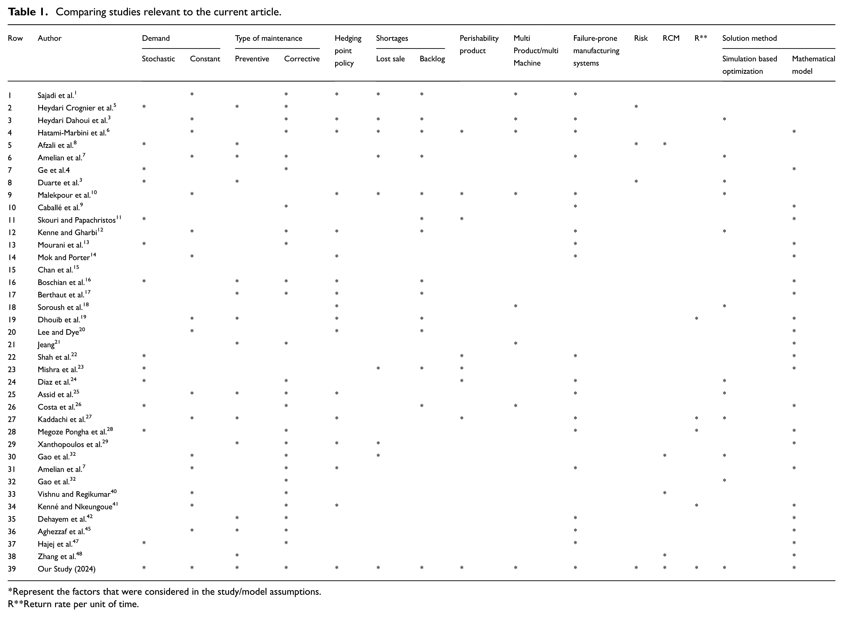
Represent the factors that were considered in the study/model assumptions.R**Return rate per unit of time.

The first point examines the types of maintenance and repair operations, including both corrective and preventive measures. The second and third points address the production strategy, which allows for inconclusive items and permits backlog and lost sales. The fourth point focuses on production control, which is often crucial in systems with uncertainties. The fifth point considers the type of production system, distinguishing between definitive and non-definitive systems. The sixth point in the comparison table compares the failure coefficient of the production unit, which is related to the unit’s lifetime. The final point in this table discusses the provision of Reliability-Centered Maintenance policies.

2.5. Identifying the knowledge gap in the literature review

2.5.1. Lack of comprehensive analysis of multiple key factors

As shown in Table 1, most previous studies have focused on specific aspects such as maintenance type, production strategies, or failure-prone manufacturing systems. However, the simultaneous integration of “failure-prone manufacturing systems modeling,”“risk analysis,”“Reliability-Centered Maintenance (RCM),” and “simulation-based optimization” has been rarely explored in prior research.

2.5.2. Insufficient comparison of maintenance strategies

While some studies, such as Amelian et al. ⁷ and Dhouib et al., ¹⁹ have analyzed maintenance strategies, a detailed comparison between RCM and other maintenance approaches and their impact on manufacturing system efficiency remains underexplored.

2.5.3. Limited integration of simulation and optimization

Some studies, such as Boschian et al. ¹⁶ and Heydari Dahoui et al., ⁵ have used simulation for system analysis. However, the combination of simulation with mathematical optimization in the context of failure-prone manufacturing systems has received little attention.

2.5.4. Lack of comprehensive risk analysis in maintenance and production decision-making

Although some studies, such as Hatami-Marbini et al. ⁶ and Kaddachi et al., ²⁷ have discussed risk in manufacturing systems, the impact of risk analysis on RCM strategies and its influence on managerial decision-making in failure-prone manufacturing environments requires further investigation.

2.6. Conclusion on the knowledge gap

This study aims to bridge these knowledge gaps by introducing a comprehensive approach that integrates mathematical modeling, simulation, and optimization for failure-prone manufacturing systems while incorporating risk analysis and RCM strategies.

3. Problem solving methodology

In this section, we will begin by discussing the problem and its mathematical relationships. We will then proceed to describe the model used in the ARENA simulation software. The model will be simulated and calculated, taking into consideration both preventive and corrective maintenance policies, as well as their performance variables. The Reliability-Centered Maintenance program will be optimized using two meta-heuristic methods and the Scatter search tool. The overall process for the system being studied in this article is shown in Figure 1.

Figure 1.

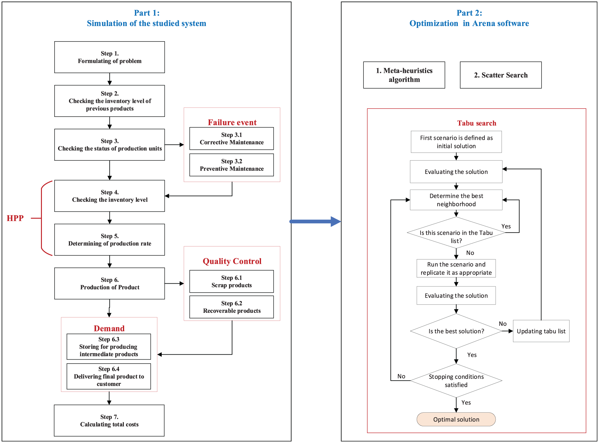
Conceptual model for conducting the article process.

Our methodology integrates Reliability-Centered Maintenance (RCM) and risk analysis into the production and maintenance planning framework. Specifically, RCM is employed to identify critical equipment and schedule preventive maintenance activities, optimizing resource allocation to minimize production failures. Risk is modeled as a dynamic metric, capturing the probability and impact of failures, and is explicitly incorporated into the production scheduling model as both a decision criterion and a constraint. This novel approach ensures a multi-dimensional analysis of the production system by linking maintenance strategies with inventory management and failure risk. For instance, RCM guides the prioritization of repairs, while risk metrics determine the optimal production and maintenance schedules under uncertainty. Such integration distinguishes our methodology from previous studies that typically address production and maintenance separately.

4. Analysis of the current maintenance procedure

The current maintenance system in the plant is predominantly reactive in nature, relying heavily on corrective maintenance actions after equipment failure. Preventive maintenance activities are minimal and not scheduled based on the actual condition or performance of the equipment. This approach has led to increased downtime, higher maintenance costs, and a lower level of production reliability. The existing maintenance records and failure logs were analyzed to identify the average time between failures (MTBF), mean time to repair (MTTR), and the frequency of breakdowns for each production unit. It was observed that the plant lacks a systematic method for prioritizing maintenance activities or allocating resources effectively. In addition, there is no integration of maintenance planning with production scheduling, which results in suboptimal operational efficiency. A gap analysis was conducted to compare the current practice with industry standards and best practices in reliability-centered maintenance (RCM). The analysis revealed that the current system does not adequately support decision-making regarding maintenance interventions or provide sufficient data to prevent critical failures. The proposed simulation model incorporates an improved maintenance strategy based on condition monitoring and preventive scheduling, aligned with RCM principles. This allows for better asset management, reduced unscheduled downtime, and optimized maintenance costs. The results of the simulation are compared against the baseline performance of the existing maintenance strategy to quantify improvements in key performance metrics such as system availability, total cost, and production output. This structured evaluation of the current maintenance approach ensures that the improvements observed in the simulation are not only meaningful but also directly attributable to the enhanced maintenance planning and execution strategies introduced in the proposed model.

5. Problem statement

This article discusses a system, depicted in Figure 2, that is susceptible to non-definitive network failure.

Figure 2.

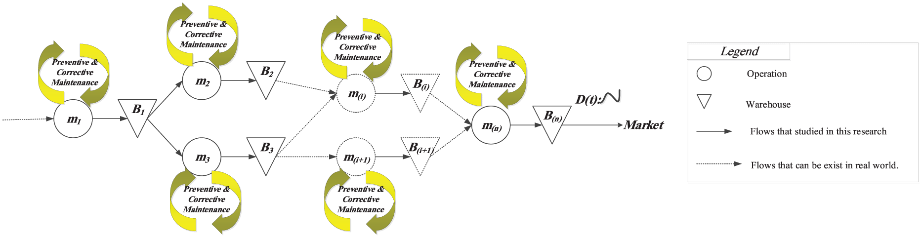
Network failure-prone manufacturing system.

This system assumes the presence of non-stable or perishable items, which are considered failures and result in the failure of the production unit. The system consists of n non-identical production units, each producing a specific type of product at different stages of production. The product produced at stage $i$ , with a consumption coefficient $\left(l_{\mathrm{ij}}\right)$ , is used in the production of the product at stage $j$ . When all production units are functioning properly, products are produced at a rate of $u_i\left(t\right)$ . These products undergo qualitative inspection and are sent to the rework department if necessary. Repairable products are sent for repairs, while products deemed irreparable are considered scrap and removed from the system. The rate at which products are returned to the reworking stage is directly linked to the lifespan of the production unit. In other words, products have a higher chance of being reworked if the production unit remains functional for a longer period of time. After each production unit, there is a warehouse where excess inventory is stored to ensure that production does not halt in the event of a failure in the previous production unit $(i-1)$ . The warehouse acts as a buffer between the failure and the demand, meaning that when a failure occurs, the current demand is met by retrieving products from the warehouse to repair the failed unit and resume production.

The failure of the production unit is bound to happen. To prevent sudden breakdowns, it is crucial to regularly visit the production unit and plan preventive maintenance. Occasionally, the production unit may fail unexpectedly, causing production to halt. In such cases, implementing a maintenance and repair program is necessary. This article assumes that performing maintenance and repair extends the lifespan of the production unit by a constant factor. However, by conducting preventive maintenance and repair, the lifespan of the production unit can be reset to the factory’s initial state. Figure 3 provides an overview of the performance of each production unit.

Figure 3.

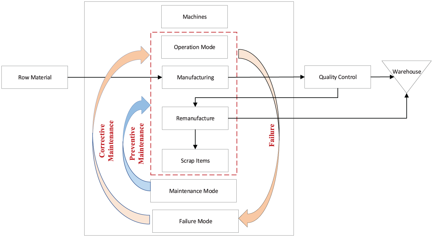
The overall performance of each production unit in the system studied.

In failure-prone manufacturing systems, equipment breakdowns can cause production delays, increased costs, and reduced efficiency. One critical factor influencing failure rates is the presence of defective and unstable products, which deteriorate production quality and lead to higher maintenance and repair demands. In such environments, implementing an efficient maintenance strategy that can predict and control failures is essential. One of the major challenges in these systems is the presence of unstable or defective products, which increase the failure rate of production units. In addition, traditional maintenance and repair methods may not be efficient in reducing costs and improving system reliability. Many previous studies have analyzed failure-prone manufacturing systems, but the role of defective products in system failure rates has been largely overlooked. Some studies have investigated Reliability-Centered Maintenance (RCM) strategies, but their comparison with other maintenance strategies in multi-stage environments remains an open research gap. Existing research has primarily examined production control in static conditions, whereas optimization and simulation approaches for dynamic production control under uncertainty have received less attention.

However, previous studies have certain limitations:

• The role of defective products in system failure rates has not been thoroughly investigated.

• The comparison of RCM with other maintenance strategies in multi-stage systems is lacking.

• Limited research has focused on integrating production control and inventory management in the presence of sudden failures.

• Multi-dimensional evaluations of system performance (including quality, cost, and repair time) have been insufficient.

This research aims to fill these gaps and pursue the following objectives:

• Develop a new mathematical model to examine the effect of defective products on system failure rates.

• Design and compare RCM with other maintenance strategies to optimize system performance.

• Utilize simulation and optimization techniques to enhance production control under uncertainty.

• Establish multi-dimensional performance metrics to evaluate system efficiency.

This model will assist production managers in making optimal decisions regarding maintenance and production planning, thereby improving the efficiency of failure-prone manufacturing systems.

5.1. Assumptions of the problem

The assumptions in this article can be summarized as follows:

• The demand for intermediate products used in the production of the next product is fixed and known, while the demand for the final product varies over time.

• The production rate is discrete.

• The model being studied is multi-product.

• The production process does not allow for backward production.

• Intermediate production units will never experience shortages of raw materials.

• A shortage of both scrap and lost sales is allowed for the final product.

• If there is insufficient stock of the intermediate stage I product (based on the consumption coefficient), the production of the next stage product will be halted and the production rate will be zero.

• The failure and repair times of all machines in the system are exponential.

• Perishable of items is allowed for the final production stage product, and if the product is not consumed by the desired date, it is considered corrupt.

• The defective commodity coefficient is dependent on the lifespan of the production unit.

• If expired items are delivered to a customer and there is a demand for expired items in the system, priority will be given to the customer who received the expired items to fulfill the demand.

• The production unit can be stopped and repaired for two reasons: preventive repairs and emergency repairs.

• The time required for repair varies depending on the type of failure, the speed of the repairmen, and other factors.

• Planning for preventive repairs also varies depending on the type of production unit and its failure records.

• At the start of the study, all machines are in a safe and operational state.

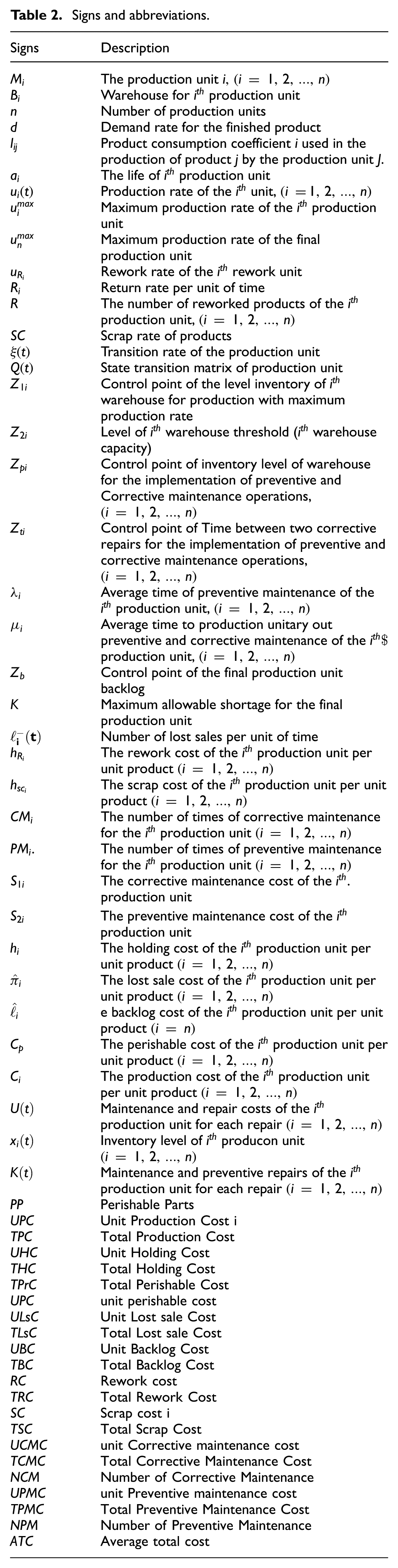
5.2. Symbols

The symbols used in the studied system modeling are shown in Table 2.

Table 2.

Signs and abbreviations.

Signs	Description
$M_i$	The production unit $i,(i=1,2,...,n)$
$B_i$	Warehouse for $i^{\mathrm{th}}$ production unit
$n$	Number of production units
$d$	Demand rate for the finished product
$l_{\mathrm{ij}}$	Product consumption coefficient $i$ used in the production of product $j$ by the production unit $J$ .
$a_i$	The life of $i^{\mathrm{th}}$ production unit
$u_i(t)$	Production rate of the $i^{\mathrm{th}}$ unit, $(i=1,2,...,n)$
$u_i^{\max }$	Maximum production rate of the $i^{\mathrm{th}}$ production unit
$u_n^{\max }$	Maximum production rate of the final production unit
$u_{R_i}$	Rework rate of the $i^{\mathrm{th}}$ rework unit
$R_i$	Return rate per unit of time
$R$	The number of reworked products of the $i^{\mathrm{th}}$ production unit, $(i=1,2,...,n)$
$\mathrm{SC}$	Scrap rate of products
$\xi (t)$	Transition rate of the production unit
$Q(t)$	State transition matrix of production unit
$Z_{1i}$	Control point of the level inventory of $i^{\mathrm{th}}$ warehouse for production with maximum production rate
$Z_{2i}$	Level of $i^{\mathrm{th}}$ warehouse threshold ( $i^{\mathrm{th}}$ warehouse capacity)
$Z_{\mathrm{pi}}$	Control point of inventory level of warehouse for the implementation of preventive and Corrective maintenance operations, $(i=1,2,...,n)$
$Z_{\mathrm{ti}}$	Control point of Time between two corrective repairs for the implementation of preventive and corrective maintenance operations, $(i=1,2,...,n)$
${\lambda }_i$	Average time of preventive maintenance of the $i^{\mathrm{th}}$ production unit, $(i=1,2,...,n)$
${\mu }_i$	Average time to production unitary out preventive and corrective maintenance of the $i^{\mathrm{th}}$ production unit, $(i=1,2,...,n)$
$Z_b$	Control point of the final production unit backlog
$K$	Maximum allowable shortage for the final production unit
${\ell }_{\mathbf{i}}^{-}\left(\mathbf{t}\right)$	Number of lost sales per unit of time
$h_{R_i}$	The rework cost of the $i^{\mathrm{th}}$ production unit per unit product $(i=1,2,...,n)$
$h_{s{c}_i}$	The scrap cost of the $i^{\mathrm{th}}$ production unit per unit product $(i=1,2,...,n)$
$C{M}_i$	The number of times of corrective maintenance for the $i^{\mathrm{th}}$ production unit $(i=1,2,...,n)$
$P{M}_i$ .	The number of times of preventive maintenance for the $i^{\mathrm{th}}$ production unit $(i=1,2,...,n)$
$S_{1i}$	The corrective maintenance cost of the $i^{\mathrm{th}}$ . production unit
$S_{2i}$	The preventive maintenance cost of the $i^{\mathrm{th}}$ production unit
$h_i$	The holding cost of the $i^{\mathrm{th}}$ production unit per unit product $(i=1,2,...,n)$
${\hat{\pi }}_i$	The lost sale cost of the $i^{\mathrm{th}}$ production unit per unit product $(i=1,2,...,n)$
${\hat{\ell }}_i$	e backlog cost of the $i^{\mathrm{th}}$ production unit per unit product $(i=n)$
$C_p$	The perishable cost of the $i^{\mathrm{th}}$ production unit per unit product $(i=1,2,...,n)$
$C_i$	The production cost of the $i^{\mathrm{th}}$ production unit per unit product $(i=1,2,...,n)$
$U\left(t\right)$	Maintenance and repair costs of the $i^{\mathrm{th}}$ production unit for each repair $(i=1,2,...,n)$
$x_i\left(t\right)$	Inventory level of $i^{\mathrm{th}}$ producon unit $(i=1,2,...,n)$
$K\left(t\right)$	Maintenance and preventive repairs of the $i^{\mathrm{th}}$ production unit for each repair $(i=1,2,...,n)$
$\mathrm{PP}$	$\mathrm{Perishable}\mathrm{Parts}$
$\mathrm{UPC}$	$\mathrm{Unit}\mathrm{Production}\mathrm{Cost}\mathrm{i}$
$\mathrm{TPC}$	$\mathrm{Total}\mathrm{Production}\mathrm{Cost}$
$\mathrm{UHC}$	$\mathrm{Unit}\mathrm{Holding}\mathrm{Cost}$
$\mathrm{THC}$	$\mathrm{Total}\mathrm{Holding}\mathrm{Cost}$
$\mathrm{TPrC}$	$\mathrm{Total}\mathrm{Perishable}\mathrm{Cost}$
$\mathrm{UPC}$	$\mathrm{unit}\mathrm{perishable}\mathrm{cost}$
$\mathrm{ULsC}$	$\mathrm{Unit}\mathrm{Lost}\mathrm{sale}\mathrm{Cost}$
$\mathrm{TLsC}$	$\mathrm{Total}\mathrm{Lost}\mathrm{sale}\mathrm{Cost}$
UBC	$\mathrm{Unit}\mathrm{Backlog}\mathrm{Cost}$
TBC	$\mathrm{Total}\mathrm{Backlog}\mathrm{Cost}$
$\mathrm{RC}$	$\mathrm{Rework}\mathrm{cost}$
$\mathrm{TRC}$	$\mathrm{Total}\mathrm{Rework}\mathrm{Cost}$
$\mathrm{SC}$	$\mathrm{Scrap}\mathrm{cost}\mathrm{i}$
$\mathrm{TSC}$	$\mathrm{Total}\mathrm{Scrap}\mathrm{Cost}$
$\mathrm{UCMC}$	$\mathrm{unit}\mathrm{Corrective}\mathrm{maintenance}\mathrm{cost}$
$\mathrm{TCMC}$	$\mathrm{Total}\mathrm{Corrective}\mathrm{Maintenance}\mathrm{Cost}$
$\mathrm{NCM}$	$\mathrm{Number}\mathrm{of}\mathrm{Corrective}\mathrm{Maintenance}$
$\mathrm{UPMC}$	$\mathrm{unit}\mathrm{Preventive}\mathrm{maintenance}\mathrm{cost}$
$\mathrm{TPMC}$	$\mathrm{Total}\mathrm{Preventive}\mathrm{Maintenance}\mathrm{Cost}$
$\mathrm{NPM}$	$\mathrm{Number}\mathrm{of}\mathrm{Preventive}\mathrm{Maintenance}$
$A\mathrm{TC}$	$\mathrm{Average}\mathrm{total}\mathrm{cost}$

5.3. Equations

5.3.1. The state of production units

The symbols represent the state of the production unit at time $t$ , which follows a semi-Markovian random process with possible values of or $i(t)=\{1,2,3\}$ . The $Q(t)$ matrix also indicates how the state of the production unit changes from each of the defined states in ${\xi }_i(t)$ . ⁵¹

$${\xi }_i\left(t\right)=\{\begin{array}{c}1i^{\mathrm{th}}\mathrm{production}\mathrm{unit}\mathrm{is}\mathrm{opertional}\hfill \\ \multicolumn{1}{c}{2i^{\mathrm{th}}\mathrm{production}\mathrm{unit}\mathrm{is}\mathrm{under}\mathrm{repair}}\\ \multicolumn{1}{c}{3i^{\mathrm{th}}\mathrm{production}\mathrm{unit}\mathrm{is}\mathrm{under}\mathrm{preventive}\mathrm{Maintenance}}\end{array}$$

(1)

$$Q\left(t\right)=\left[\begin{array}{ccc}-(q_{12i}\left(a_i\right)+q_{13i})\hfill & q_{12i}{a}_i\hfill & q_{13i}\hfill \\ \multicolumn{1}{c}{q_{21i}}& -q_{21i}\hfill & 0\hfill \\ \multicolumn{1}{c}{q_{31i}}& 0\hfill & -q_{31i}\hfill \end{array}\right]$$

(2)

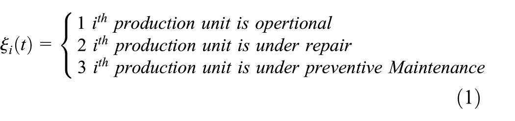
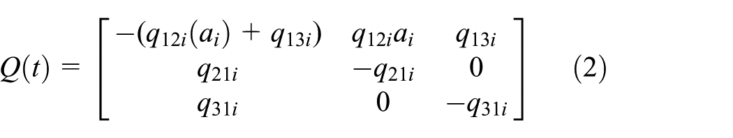
As mentioned in the signs and abbreviations section, $a_i$ represents the life of the ${\mathrm{i}}^{\mathrm{th}}\mathrm{production}\mathrm{unit}\mathrm{is}\mathrm{opertional}$ production unit. The failure of the production unit is dependent on its life, which increases as the unit ages. The failure occurs at a rate of $q_{12i}\left(a_i\right)$ , which also increases with the age of the unit. When a failure occurs, the unit undergoes corrective repair and returns to operational mode. Maintenance and repair operations are also necessary to address bottlenecks, system decline, and restore the unit’s life even when it is functioning properly. Preventive maintenance and repair bring the age of the unit back to zero. The failure rate, $q_{21i}$ , indicates the transition from operational to production unit failure and is determined by the age of the unit. Transitioning from operational mode to preventive maintenance and repair mode only occurs when the system is operating, which means $q_{23i}=0$ . Consequently, after maintenance and preventive operations, it is not possible to transition to Mode 2, which involves unit failure and corrective repair operations ( $q_{32i}=0$ ).

5.3.2. Production rates equations

The production rate of each production unit varies depending on whether it is operational or under repair. The equations for calculating the production rates are as follows:

$$u_i\left(t\right)=\{\begin{array}{c}0\mathrm{If}{\mathrm{i}}^{\mathrm{th}}\mathrm{production}\mathrm{unit}\mathrm{is}\mathrm{under}\mathrm{repair}\hfill \\ \multicolumn{1}{c}{[0,U_{\max }]\mathrm{If}{\mathrm{i}}^{\mathrm{th}}\mathrm{production}\mathrm{unit}\mathrm{is}\mathrm{opertional}}\end{array}$$

(3)

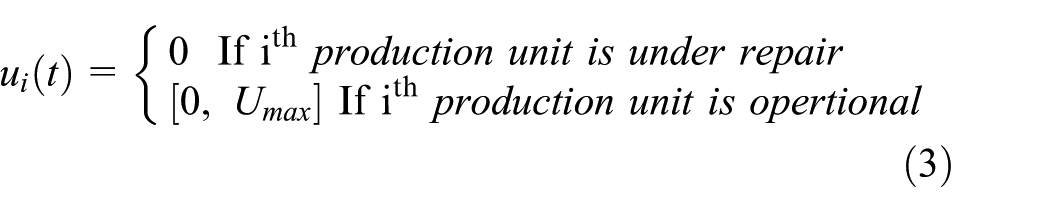
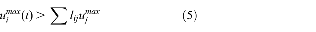
5.3.3. Maximum rate of production

In this article, it is stated in equation (4) that the production process does not allow for forward and backward movement. When the production unit undergoes repair, i.e., $u_i\left(t\right)=0$ , production is halted and the production rate becomes zero. However, if the production unit is in good condition and there is a demand for the desired product, as well as enough storage capacity in the production unit’s warehouse, the production rate will fluctuate between zero and the machine’s maximum production capacity. Each production unit has a defined maximum production rate, which is determined by equations (5) and (6). These Equations establish the conditions for system stability and the ability to meet the demands of intermediate production units, as well as the final production unit’s product demand. ¹

$$l_{\mathrm{ij}}=0\mathrm{if}j<i$$

(4)

$$u_i^{\max }(t)>\sum l_{\mathrm{ij}}{u}_j^{\max }$$

(5)

$$u_n^{\max }(t)>d$$

(6)

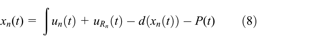
5.3.4. Inventory level

Equations (7) and (8) define the inventory level of the intermediate production unit’s products and the final production unit’s products, respectively. In addition, equation (9) represents the inventory amount that is returned to the reworking phase.

$$\begin{array}{c}\multicolumn{1}{c}{x_i(t)=\int (u_i\left(t\right)+u_{R_i}\left(t\right)}\\ \multicolumn{1}{c}{-\sum _{j>i}{l}_{\mathrm{ij}}{u}_i(t))\mathrm{dt},x_i\left(0\right)=x_i^0,1\le i<n,}\\ \multicolumn{1}{c}{x_i\left(t\right):\mathrm{integer}}\end{array}$$

(7)

$$x_n(t)=\int u_n\left(t\right)+u_{R_n}\left(t\right)-d\left(x_n\left(t\right)\right)-P(t)$$

(8)

$$x_R(t)=R_i-u_{R_i}(t)$$

(9)

$$x_i(t)\ge 0$$

(10)

$$d\left(x_n\left(t\right)\right)=\{\begin{array}{c}\begin{array}{cc}d\hfill & x_n\left(t\right)\ge -K\hfill \end{array}\hfill \\ \multicolumn{1}{c}{\begin{array}{cc}0\hfill & \mathrm{Otherwise}\hfill \end{array}}\end{array}$$

(11)

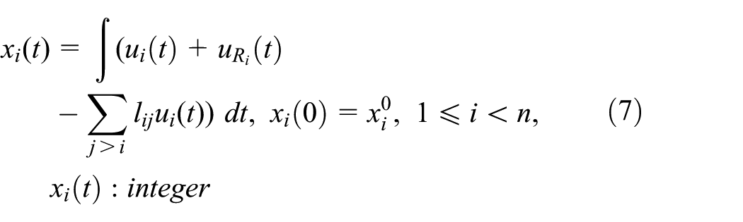
The limitations of inventory levels for the intermediate production units and the final production units product in the warehouses are expressed in the following equations, respectively.

$$-K\le x_n\left(t\right)\le Z_{2n}$$

(12)

$$0\le x_i\left(t\right)\le Z_{2i}i\ne n$$

(13)

Equation (12) states that only the shortage of $K$ units of a specific type of scrap are allowed, and any excess demand is treated as lost sales. However, this rule does not apply to the middle warehouses.

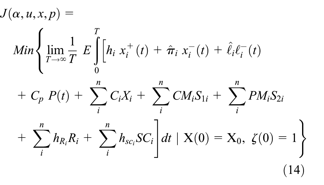
The objective function of the problem described below aims to minimize the mathematical expectation of the total cost per unit time. This includes production costs, maintenance costs, shortage costs (including lost sales and retention), repair costs (both corrective and preventive), costs of reworking, and costs of items Perishable.

$$J\left(\alpha ,u,x,p\right)=\left\{Min\underset{T\to \infty }{\lim }\frac{1}{T}E\underset{0}{\overset{T}{\int }}\left[h_i{x}_i^{+}\left(t\right)+{\widehat{\pi }}_i{x}_i^{-}\left(t\right)+{\widehat{\ell }}_i{\ell }_i^{-}\left(t\right)+C_{p}P\left(t\right)+\sum _i^n{C}_i{X}_i+\sum _i^{n}C{M}_i{S}_{1i}+\sum _i^{n}P{M}_i{S}_{2i}+\sum _i^n{h}_{R_i}{R}_i+\sum _i^n{h}_{s{c}_i}S{C}_i\right]dt|\mathrm{X}\left(0\right){=\mathrm{X}}_0,\zeta \left(0\right)=1\right\}$$

(14)

$$x_i^{-}\left(t\right)=\mathrm{Max}(-x_i\left(t\right),0)$$

(15)

$${\ell }_i^{-}\left(t\right)=\mathrm{Max}(\mathrm{lost}\mathrm{sale},0)$$

(16)

5.3.5. Determining the age of the production unit

Within this system, the age of the production unit is determined by the level of production. As production increases, the age of the production unit also increases based on a specific coefficient, indicated by equation (17).

$$a_i(t)=k{u}_i(t)$$

(17)

5.3.6. Production control policy

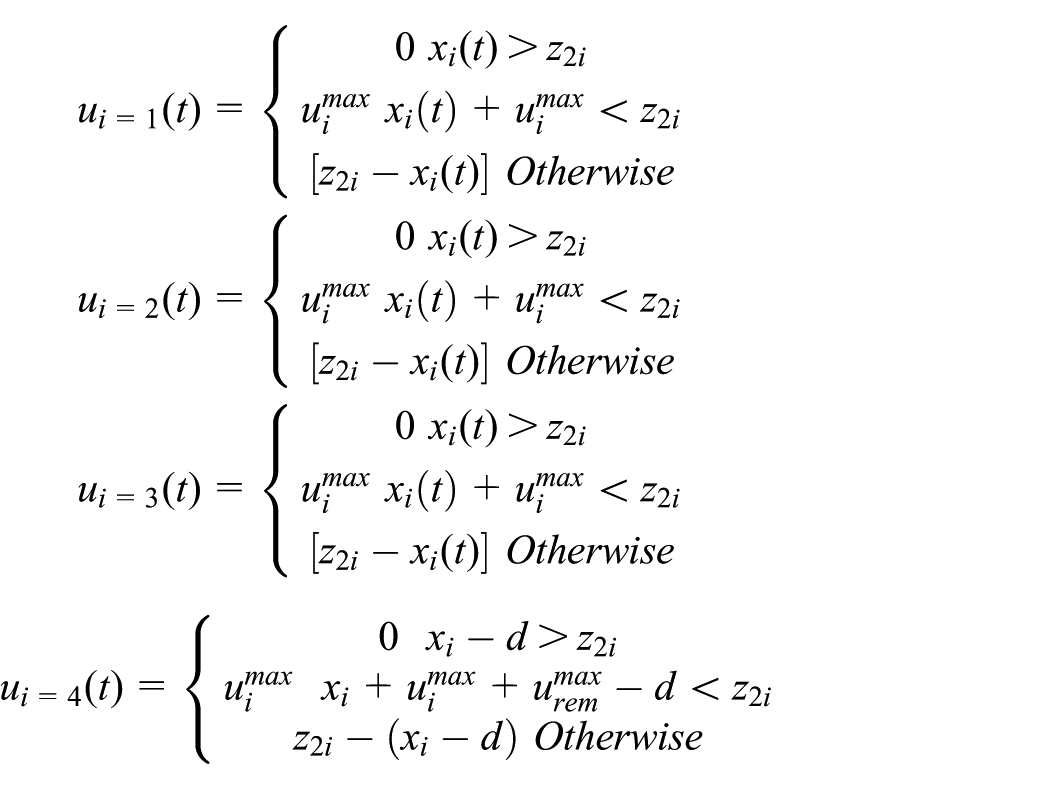
Planning production systems that are vulnerable to failure can be a highly intricate task. Rishel ⁵² has demonstrated that the optimal solution for such systems lies in the paired solution of the Hamilton-Jacoby Bellman equations. In cases where analytical solutions are not available for complex systems, the limiting point policy can be employed to minimize the objective function of the problem. This policy is straightforward to understand and execute. The control policy outlined in this article is as follows:

$$u_{i\ne n}(t)=\{\begin{array}{c}0x_i(t)>z_{2i}\hfill \\ \multicolumn{1}{c}{u_i^{\max }{x}_i\left(t\right)+u_i^{\max }<z_{2i}}\\ \multicolumn{1}{c}{[z_{2i}-x_i(t)]\mathrm{Otherwise}}\end{array}$$

(18)

$$u_{i=n}(t)=\{\begin{array}{c}0x_i-d>z_{2i}\hfill \\ \multicolumn{1}{c}{u_i^{\max }{x}_i+u_i^{\max }+u_{\mathrm{rem}}^{\max }-d<z_{2i}}\\ \multicolumn{1}{c}{z_{2i}-(x_i-d)\mathrm{Otherwise}}\end{array}$$

(19)

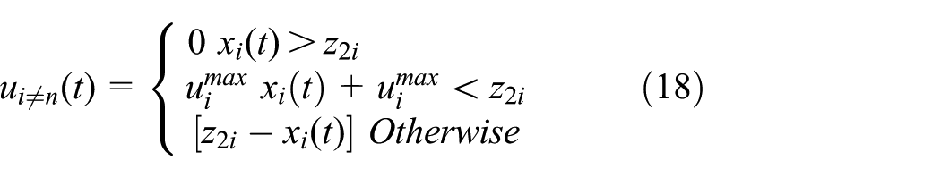
The production rate of each production unit is determined by $z_{2i}$ , which represents the inventory threshold level of each warehouse. Therefore, z_2i is defined as the decision variable. ⁵³

5.3.7. Decision variables

At each stage of production five control points $z_{1i}$ , $z_{2i}$ , $z_{\mathrm{p}i}$ , $z_{\mathrm{t}i}$ and $z_{\mathrm{b}}$ we have. $z_{1i}$ means that if the inventory level of the ith production unit reaches $z_{1i}$ , the system produces with maximum production power. $z_{2i}$ is the maximum warehouse capacity of the ith production unit. $z_{\mathrm{p}i}$ point control, maintenance and repairs, is that if the level of inventory production unit ith to $z_{\mathrm{p}i}$ reach and the time between the two repairs revamped its production unit also $z_{\mathrm{t}i}$ be reached preventive maintenance is that in terms of logical $z_{1i}$ have the following $z_{\mathrm{p}i}$ be. There is another variable called $z_{\mathrm{b}}$ , which is the control point of the backlog shortages.

5.3.8. Objectives

The purpose of this article is to reduce the average total cost of production through various strategies such as maintenance, repair, preventive maintenance, and the prevention of backlogs, lost sales, rework, scrap, and Perishable of items. In previous studies, there has been a lack of consideration for selecting the best maintenance policy that takes into account both reliability and optimization of production while also considering existing risks such as unstable items, production unit failures, non-definite network systems, and various restrictions such as limited warehouse capacity and production capacity. This article aims to fill that gap and provide new insights.

The mathematical formulation introduces a novel parameter, failure rates, which explicitly captures the probabilistic impact of defective products on the production failure rate. Unlike previous studies that assume deterministic failure rates, our model incorporates dynamic interactions between maintenance strategies and inventory levels. In addition, the optimization framework employs a hybrid approach, combining stochastic and deterministic methods to enhance solution accuracy and computational efficiency. Also, the mathematical formulation also incorporates a novel parameter, $R_i$ , which captures the probabilistic rate of rework associated with defective products. This addition highlights the dynamic relationship between the failure rate and the rework process, addressing the iterative feedback loop between production quality and maintenance strategies. Unlike previous studies that treat rework rates as constant or negligible, our model accounts for how variations in production conditions and maintenance efforts influence rework rates over time. Combined with failure rate this comprehensive approach enables a more accurate depiction of the interplay between maintenance, inventory, and production dynamics. The mathematical formulation also integrates the principles of Reliability-Centered Maintenance (RCM) into the optimization framework. By incorporating failure rates and the model enables the evaluation of maintenance policies based on their ability to minimize system failures and rework rates. Unlike conventional maintenance strategies, which often apply uniform or reactive approaches, RCM considers the criticality and reliability of each production unit to prioritize preventive and corrective actions. This allows the model to dynamically adjust maintenance schedules and inventory levels, optimizing the system’s overall performance. The hybrid optimization approach further ensures that RCM policies are evaluated in scenarios with varying levels of uncertainty, enhancing both the practical applicability and robustness of the proposed framework. Previous models typically relied on fixed inventory levels or traditional maintenance policies, whereas our model introduces dynamic and adjustable variables. Many studies have focused on a single aspect of the system, such as production or maintenance. In contrast, our model considers the multi-dimensional interaction between production, maintenance, and inventory.

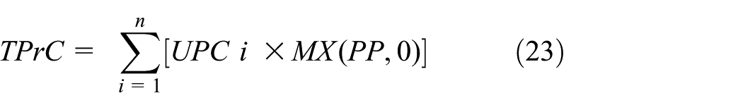
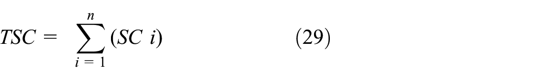
5.3.9. Total production cost

To calculate system costs, we need to consider production costs, maintenance costs, shortages (such as loss and lost sales), Perishable, rework, scrap, and maintenance and repair costs. These costs should be calculated separately for each occurrence of maintenance, corrective repairs, and preventive repairs. After calculating the individual costs for each category, we can then determine the total cost for each. Finally, the total cost of the system is determined based on the specific problem objective.

The production cost is defined as the cost of producing one unit of a product $i$ , which is then included in the overall production cost of the product $i$ . After that, the total production costs are added together and the average is calculated over time.

$$P{C}_i=P{C}_i+C_i$$

(20)

$$\mathrm{TP}{C}_i=\sum _{i=1}^n(P{C}_i)$$

(21)

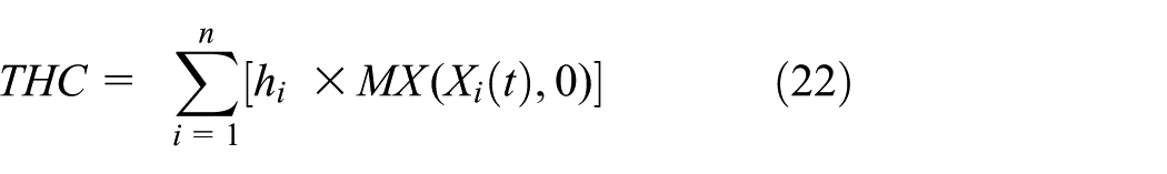
5.3.10. Total holding cost

To calculate the total holding cost for a product, follow these steps:

1. Multiply the maximum inventory in the warehouse at any given time by the cost associated with maintaining the product.

2. Add together the costs of maintaining the product for each process.

3. Calculate the average cost during the simulation period.

$$\mathrm{THC}=\sum _{i=1}^n[h_i\times \mathrm{MX}(X_i\left(t\right),0)]$$

(22)

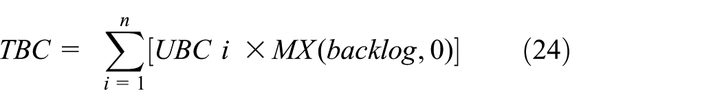
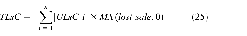
5.3.11. Perishable and shortage costs

The cost of perishable and shortages, which includes the cost of shortages and lost sales, is calculated in a similar manner as the maintenance cost. These costs are expressed using the following equations:

$$\mathrm{TPrC}=\sum _{i=1}^n[\mathrm{UPC}i\times \mathrm{MX}(\mathrm{PP},0)]$$

(23)

$$\mathrm{TBC}=\sum _{i=1}^n[\mathrm{UBC}i\times \mathrm{MX}(\mathrm{backlog},0)]$$

(24)

$$\mathrm{TLsC}=\sum _{i=1}^n[\mathrm{ULsC}i\times \mathrm{MX}(\mathrm{lost}\mathrm{sale},0)]$$

(25)

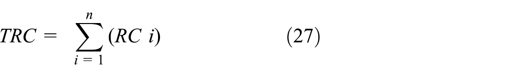
5.3.12. Rework and scrap costs

The calculation of rework costs and scrap costs is as follows: when a unit of product $i$ reaches the rework stage or is considered scrap, its cost is included in the total rework and scrap cost. The total rework and scrap costs are then added together separately, and the time average is calculated.

$$\mathrm{RC}i=\mathrm{RC}i+\mathrm{URC}i$$

(26)

$$\mathrm{TRC}=\sum _{i=1}^n(\mathrm{RC}i)$$

(27)

$$\mathrm{SC}i=\mathrm{SC}i+\mathrm{USC}i$$

(28)

$$\mathrm{TSC}=\sum _{i=1}^n(\mathrm{SC}i)$$

(29)

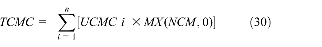
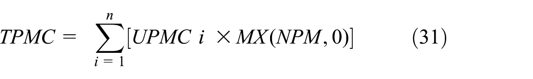
5.3.13. Corrective and preventive maintenance costs

The cost of maintenance and repair depends on how often both corrective and preventive maintenance operations are performed. Therefore, the cost of maintenance is calculated for each instance when maintenance and repair are not production unit out or when the production unit needs to be stopped for preventive maintenance and repair. Finally, the average time is used to calculate the total cost.

$$\mathrm{TCMC}=\sum _{i=1}^n[\mathrm{UCMC}i\times \mathrm{MX}(\mathrm{NCM},0)]$$

(30)

$$\mathrm{TPMC}=\sum _{i=1}^n[\mathrm{UPMC}i\times \mathrm{MX}(\mathrm{NPM},0)]$$

(31)

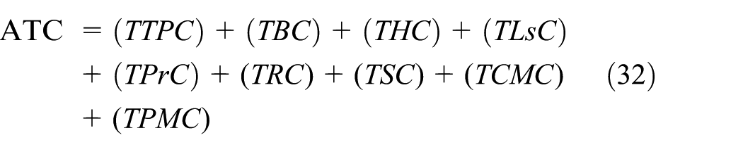
To calculate the total cost of the system, we need to consider several factors. These include the data from the static module, average production, maintenance costs, shortages and perishable costs, rework and scrap, as well as maintenance and repair costs. All of these costs are calculated and combined over a certain period of time. The overall cost of the system can be calculated using the equation provided in the ARENA software.

$$\begin{array}{c}\multicolumn{1}{c}{\mathrm{ATC}=\left(\mathrm{TTPC}\right)+\left(\mathrm{TBC}\right)+\left(\mathrm{THC}\right)+\left(\mathrm{TLsC}\right)}\\ \multicolumn{1}{c}{+\left(\mathrm{TPrC}\right)+(\mathrm{TRC})+(\mathrm{TSC})+(\mathrm{TCMC})}\\ \multicolumn{1}{c}{+(\mathrm{TPMC})}\end{array}$$

(32)

6. Simulation modeling

Simulation is an effective tool for solving complex problems related to failure-prone systems with uncertainty. This article presents a simulation study of a hypothetical system, conducted in three different sizes: small (with four production units), medium (with six production units), and large (with ten production units). The simulation was performed using ARENA 14.0 software. The stages of the simulation process for the network failure-prone system are described in eight separate stages.

6.1. Defining variables and model parameters

During the initial stages of simulation modeling, the parameters and variables of the assumed model are established. The values of variables, such as the decision of the five-point control $z_{1i}$ , $z_{2i}$ , $z_{\mathrm{p}i}$ , $z_{\mathrm{t}i}$ and $z_{\mathrm{b}}$ , are defined and initialized before the modeling process begins. Throughout the simulation, these values are modified using the Tabu search algorithm. Additional variables in the model, including the total cost of inventory maintenance, the total cost of production unit, the total cost of production, and the Perishable of items, are also defined and their values determined during the simulation.

The system parameters are universal parameters that remain constant throughout the simulation, regardless of the scenario. These parameters encompass various aspects such as the demand rate for the finished product, the consumption coefficient of the intermediate production unit, maintenance costs, shortages, Perishable, production per unit of the product in each period, and the initial inventory of the warehouse.

The model simulation for each production unit consists of three stages. These stages involve simulating the production line, followed by simulating maintenance and preventive repairs. Finally, maintenance and corrective repairs are simulated for each production unit individually.

Entry of parts. Each entity’s entry marks the start of a production process during each simulation period. Parts are introduced into the system, specifically into each production unit, at a constant rate of $u_i^{\max }$ , measured in minutes. Therefore, the time interval between two consecutive entries is equal to $\frac{1}{u_i^{\max }}$ .

$$\mathrm{Time}\mathrm{Between}\mathrm{Arrival}=\frac{1}{u_i^{\max }}$$

(33)

6.2. Production of intermediate products

After setting up the institution and entering the necessary parts, the model variables are defined. Then, the production unit mode is examined. If the production unit is undergoing corrective or preventive repair, production is halted and the part is removed from the system. If not, the availability of all materials (i.e., the amount of stage $i$ products required to produce a unit of product $j$ is checked before production begins. If there is insufficient stock on hand, production stops. Otherwise, it continues. At this point, three scenarios can occur based on the control policy defined in equation (18):

1. If the inventory at Time $t$ , ( $x_i(t)$ ), exceeds the warehouse capacity $z_{2i}$ , production stops and no further production takes place.

2. If the relationship $x_i\left(t\right)+u_i^{\max }$  <  $z_{2i}$ holds, production is production unit out at maximum capacity.

3. Otherwise, production occurs at the rate $[z_{2i}-x_i(t)]$ .

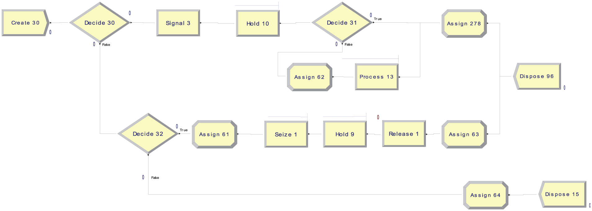
Once the production process is completed, the production unit obtains the necessary resources and releases them after a delay in the production of items. The delay is constant and its duration is equal to the reciprocal of the production rate, measured in minutes. This represents the time between the production of two items. After production, a unit is added to the warehouse inventory. Figures 4 –6 display the simulation model for the production process of intermediate products.

Figure 4.

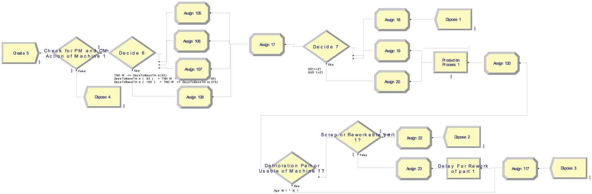
Simulation modeling for the first production unit.

Figure 5.

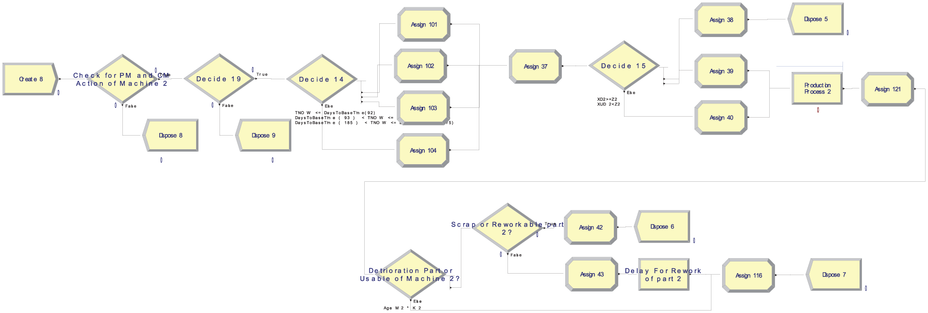
Simulation modeling for the second production unit.

Figure 6.

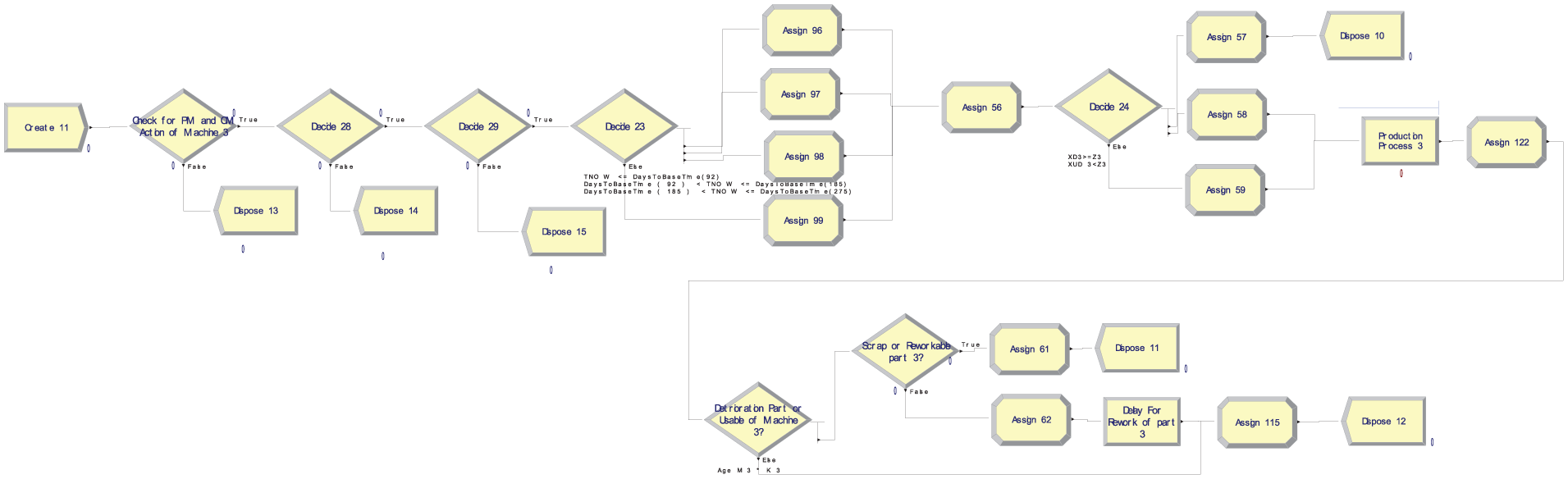
Simulation modeling for the third production unit.

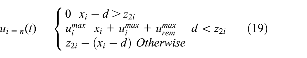
6.3. Production of the final product

The process of producing the final product is similar to producing intermediate products, with the exception that the control policy used is calculated according to equation (19). As a result, the following three scenarios may occur:

1. If the current inventory exceeds the warehouse capacity ( $z_{2i}$ ) at the time $t$ minus demand $(x_i-d>z_{2i})$ , no production will occur.

2. Production will be production unit out at maximum capacity if the relationship $x_i+u_i^{\max }+u_{\mathrm{rem}}^{\max }-d<z_{2i}$ is met.

3. Otherwise, the production process will continue at a rate of $[z_{2i}-(x_i-d)]$ .

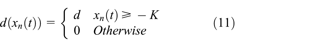
There is another difference between this stage of production and the production of intermediate products, and it relates to deterioration items. After the final product is made, the time it enters the warehouse is recorded. When a customer makes an order, the production unit is taken from the warehouse to meet the demand. If the items that are taken out have been stored in the warehouse for longer than the specified period, they are considered expired and cannot be used anymore. Otherwise, the product is considered to be in good condition. The deteriorate item is then checked. Figure 7 shows the process of producing the final product.

Figure 7.

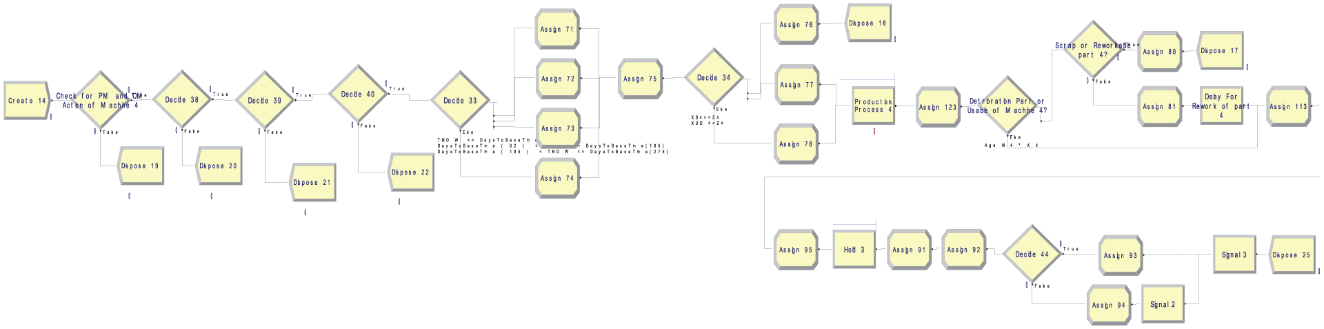
Simulation modeling for the final production unit.

6.4. Customer entry, demand, and shortage of supply process

The system facilitates customer entry and the process of fulfilling their demands. When a customer logs in, the warehouse inventory is checked using two modes:

1. If the warehouse has inventory available, a signal is sent to release the items for the final stage of production. The customer then waits for the product to be received and delivered. Upon receiving the items, if they are in good condition, the customer exits the system, and both the inventory of healthy items and the inventory of the final product are reduced. In case the delivered product is damaged, the customer remains in the system, waiting to receive a replacement.

2. If the warehouse does not have enough stock, customers have to wait for the items to be produced and received. If the number of customers in the queue exceeds a certain limit $(k)$ , new customers are not allowed to join the queue and are directed to leave the system.

It is important to note that customers who receive expired items are treated similarly to those who face a shortage of items. Both types of customers wait in line for the items to be produced. They then receive their items and exit the system in order of priority.

For further details on the demand process, please refer to Figure 8.

Figure 8.

Simulation modeling for the demand of final production unit.

6.5. Implementation of maintenance and repair policy

Implementation of maintenance and repair policy aims to highlight the importance of planning for maintenance, improve productivity, address bottlenecks caused by production unit failures, and enhance operational and product/service quality. In this system, the failure of a production unit depends on its age and production rate. Over time, the number of stochastic breakdowns increase, necessitating more maintenance and repair work. When a production unit breaks down, production is halted and corrective repair operations are initiated. Once maintenance and repair are completed, the production unit is reintegrated into the production process.

One of the objectives of this system is to schedule preventive maintenance at specific intervals. If a production unit is undergoing maintenance and corrective repairs, it is temporarily removed from the system. This means that preventive maintenance and repairs are not production unit out during this time, unless the production unit has suffered stochastic damage. However, if the desired production unit is available and production is temporarily suspended, preventive maintenance and repair operations will be executed, and the next scheduled time will be awaited. By conducting preventive maintenance and repairs, the lifespan of the production unit is effectively reset to zero, restoring the machine or production unit to its original factory state. Figure 9 illustrates corrective and preventive maintenance.

Figure 9.

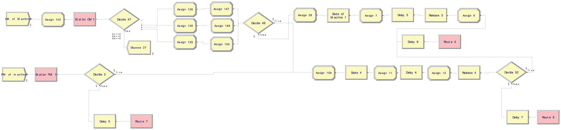
Simulation modeling for the maintenance and repair policy.

7. Accuracy of the model

In this section of the article, we aim to assess the validity and reliability of the model being studied, which is a crucial aspect of modeling and simulation. The purpose of this assessment is to compare the model with our mental model through computer simulation, allowing us to determine its level of accuracy.

First, we examine whether the model is correctly defined in the computer code. Second, we assess whether the computer code accurately represents the logical structure of the model and its input parameters. To address these questions, we have created flow diagrams for each scenario. These diagrams outline all the necessary actions and steps, building upon the information presented in the previous section. The scenarios cover various aspects, including product production during construction, final product production, production unit failure, maintenance and preventive repairs, customer arrival, and items Perishable that shown in Figures 10 –14.

Figure 10.

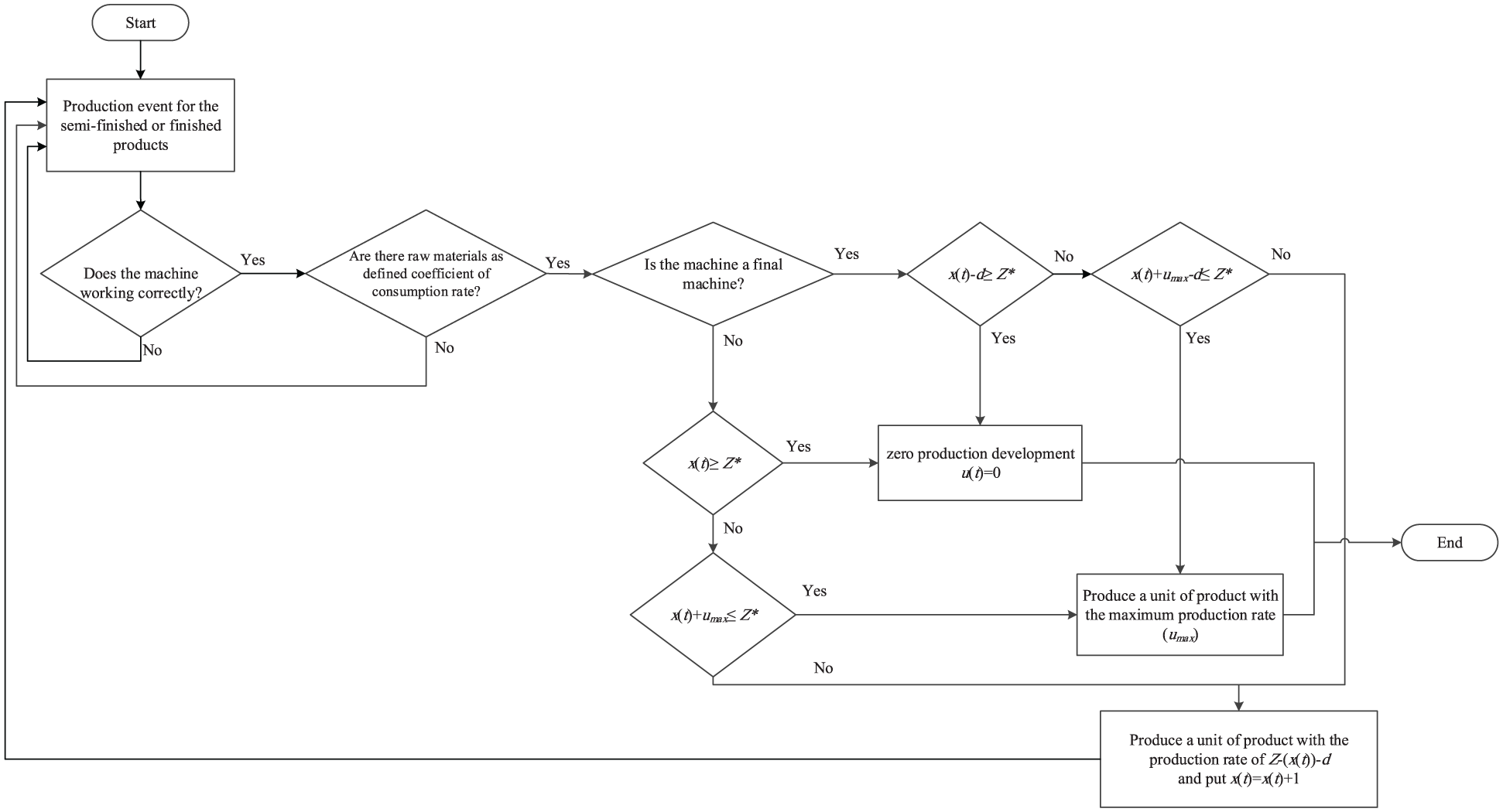
Flow diagram of product production in the manufacturing process.

Figure 11.

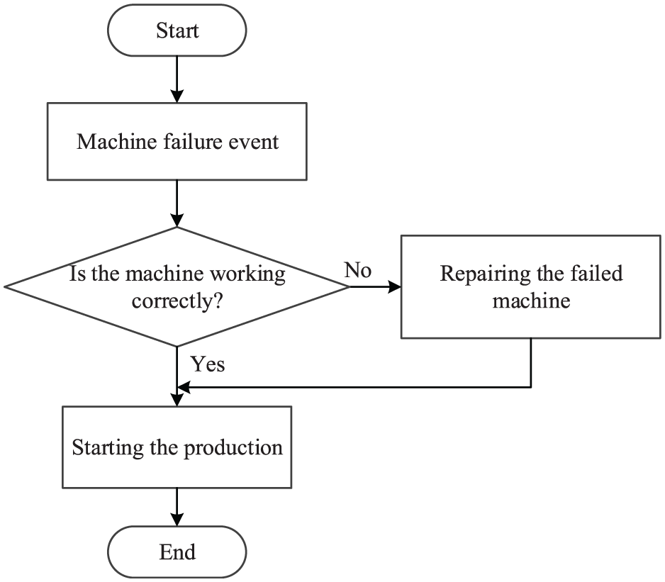
Breakdown flow diagram of the production unit.

Figure 12.

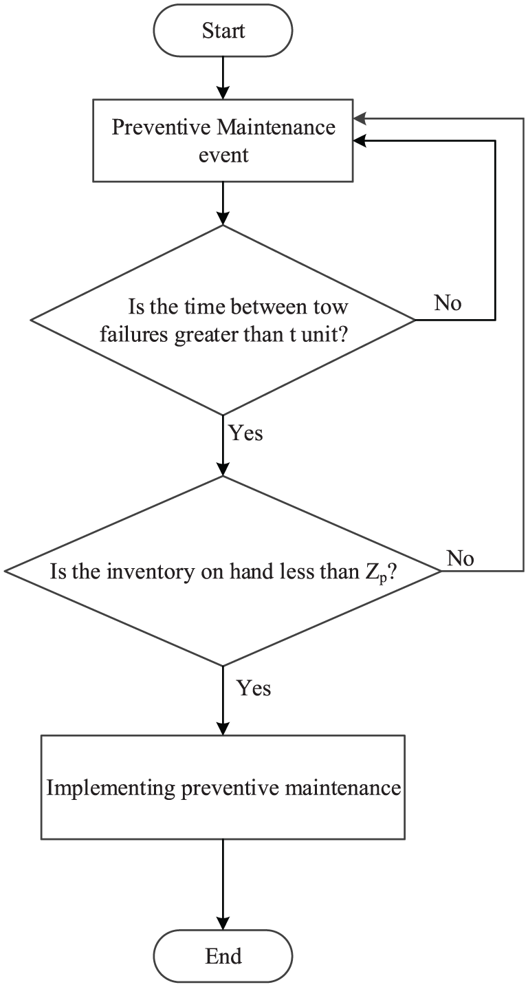
Preventive maintenance and repair procedures flow diagram.

Figure 13.

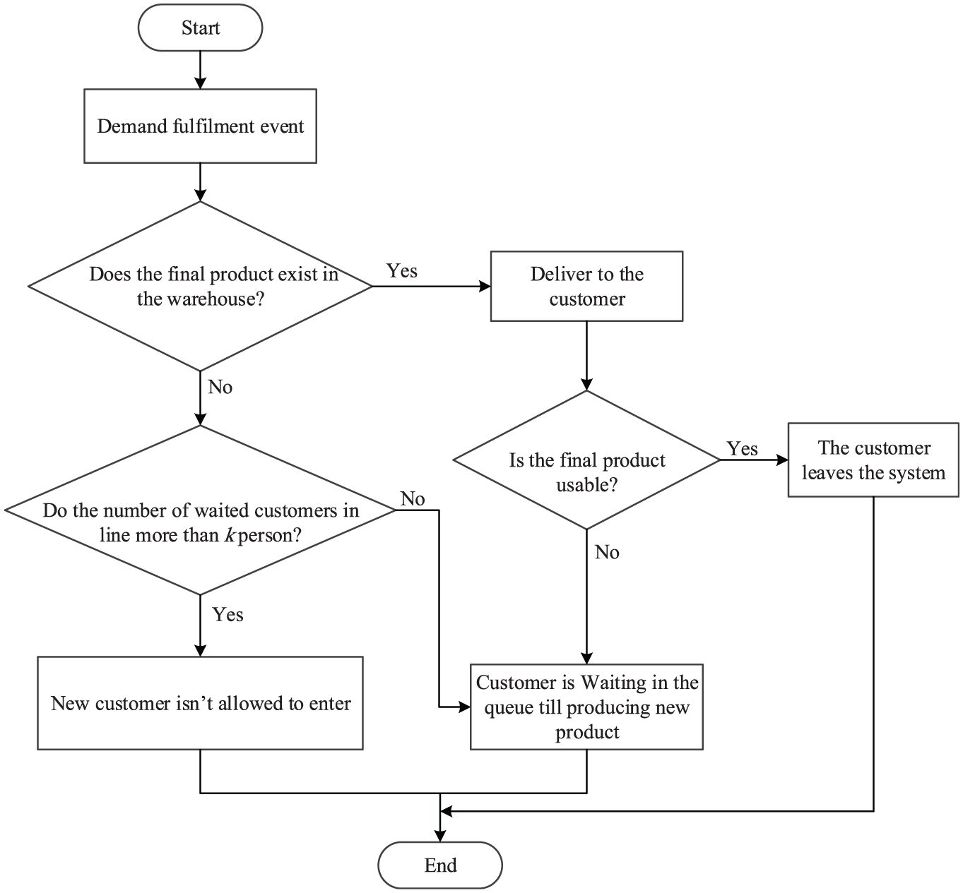
Customer login flow diagram.

Figure 14.

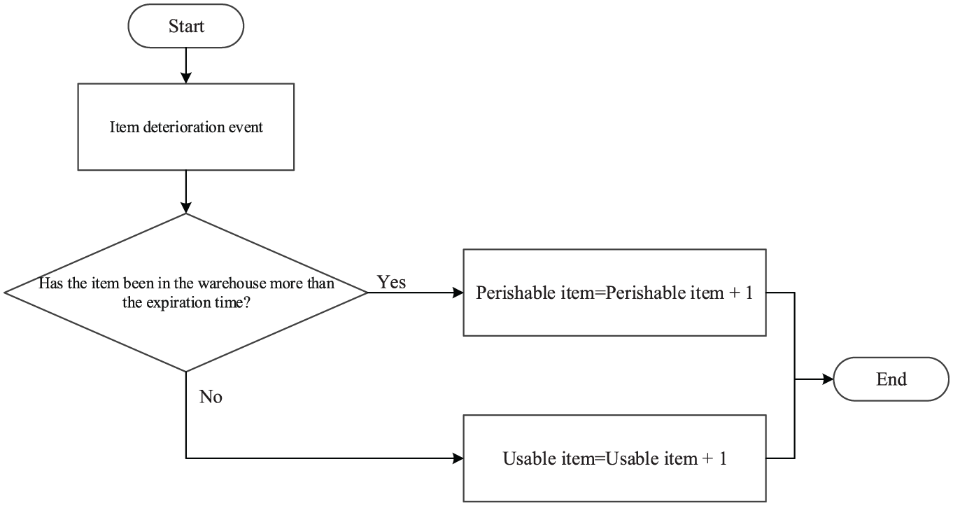
The case of product perishable.

The model’s rationality is thoroughly examined by considering multiple input parameters and ensuring the direction of institutional movement. After the simulation, all input parameters are production unit reviewed to prevent any changes. Moreover, during the implementation of the model, the Equations provided in this chapter, including the evaluation of production rates, are utilized to ensure institutions stay on the right track.

8. Validation

The validity of a simulation model is crucial because it directly impacts the decisions based on its results. To determine the validity of a model, its simulated behavior is compared to the actual behavior of the system. This process involves continuously adjusting the model to accurately reflect the real system. Various tests, both subjective and objective, are used to compare the model to reality. Subjective tests involve experts evaluating the system’s input and output, while objective tests require data on the system’s behavior and corresponding data from the model.

In the context of model validation, Naylor and Finger ⁵⁴ proposed a widely used three-step method. ⁵⁵ The procedure is as follows.

8.1. Step 1—designing the visual model

The primary objective of a simulation model designer is to ensure that the model is logical and understandable to its users. Sensitivity analysis is employed for this purpose. For example, if the customer login rate is changed, it is expected to affect the queue length. The model can also be used to analyze other sensitivities, such as the impact of changing production unit consumption coefficients and initial inventory on overall costs. Increasing the customer entry rate visually shows a decrease in queue length. In addition, changes in consumption coefficients have a significant effect on overall costs.

8.2. Step 2—assessing model assumptions

Model assumptions can be categorized into two main types: structural assumptions and data-related assumptions. Structural assumptions deal with issues related to system performance and often involve simplifying and abstracting reality. For example, in this model, it is assumed that customers who receive defective items are given priority in the queue over customers with pending orders, and they form a separate queue. This assumption is based on practical observations of the organization’s policies. Assumptions about data should be based on reliable data compilation and proper statistical analysis. If the data being collected is from a real system, consulting with system administrators and using objective statistical tests can increase the reliability of the data. In the case of Arna-assisted simulation, assumptions about production unit failures and the creation of a shared queue for customers using data and main modules are possible. In this article, all the assumptions of the hypothetical system have been translated from mathematical language into Arna simulation language.

8.3. Step 3—assessing the accuracy of input-to-output conversions

The final evaluation of the model, and essentially the only objective evaluation, is to determine whether the model, when provided with actual data as inputs and implementing the designated policy, is able to predict the future behavior of the real system. In this article, the simulation model’s outputs are calculated manually using the specified inputs, and the behavior of the simulated system is then examined based on these outputs. The results demonstrate that the obtained responses align with those of the simulated model.

8.4. Assessing model validity through statistical analysis

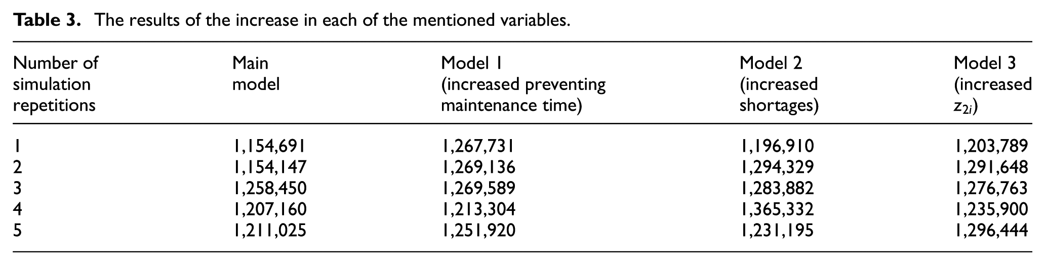
To ensure the statistical validity of the proposed model, three variables—maintenance time, permissible shortage, and warehouse level—were analyzed. The objective was to determine whether changes in these variables caused a statistically significant difference in total costs, as observed through simulation results. A paired t-test, with a 95% confidence level, was employed for this purpose. The simulation results for each variable are presented in Table 3.

Table 3.

The results of the increase in each of the mentioned variables.

Number of simulation repetitions	Main model	Model 1 (increased preventing maintenance time)	Model 2 (increased shortages)	Model 3 (increased $z_{2i}$ )
1	1,154,691	1,267,731	1,196,910	1,203,789
2	1,154,147	1,269,136	1,294,329	1,291,648
3	1,258,450	1,269,589	1,283,882	1,276,763
4	1,207,160	1,213,304	1,365,332	1,235,900
5	1,211,025	1,251,920	1,231,195	1,296,444

8.4.1. F-test for equal variances

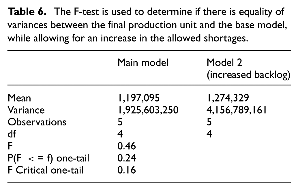
Before performing the paired t-tests, an F-test was conducted to confirm the assumption of equal variances between the two groups in each comparison. The hypotheses for the F-test are as follows:

• Null hypothesis (H₀): The variances of the two groups are equal $({\sigma }_1={\sigma }_2)$ .

• Alternative hypothesis (H₁): The variances of the two groups are not equal $({\sigma }_1\ne {\sigma }_2)$ .

$$\{\begin{array}{c}{H}_0:{\sigma }_1={\sigma }_2\hfill \\ \multicolumn{1}{c}{H_1:{\sigma }_1\ne {\sigma }_2}\end{array}$$

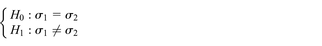
Table 4 provides the F-test results comparing variances between the base model and the model with increased maintenance and preventive maintenance time. Since the P-value (0.14) is greater than 0.05, the assumption of equal variances is accepted. Thus, it is valid to proceed with the paired t-test.

Table 4.

The F-test examines the equality of variances between the production units with increased maintenance and repair time and the base model.

	Main model	Model 1(increased preventing maintenance time)
Mean	1,197,095	1,254,336
Variance	1,925,603,250	580,137,108
Observations	5	5
df	4	4
F	3.32
P(F <= f) one-tail	0.14
F Critical one-tail	6.39

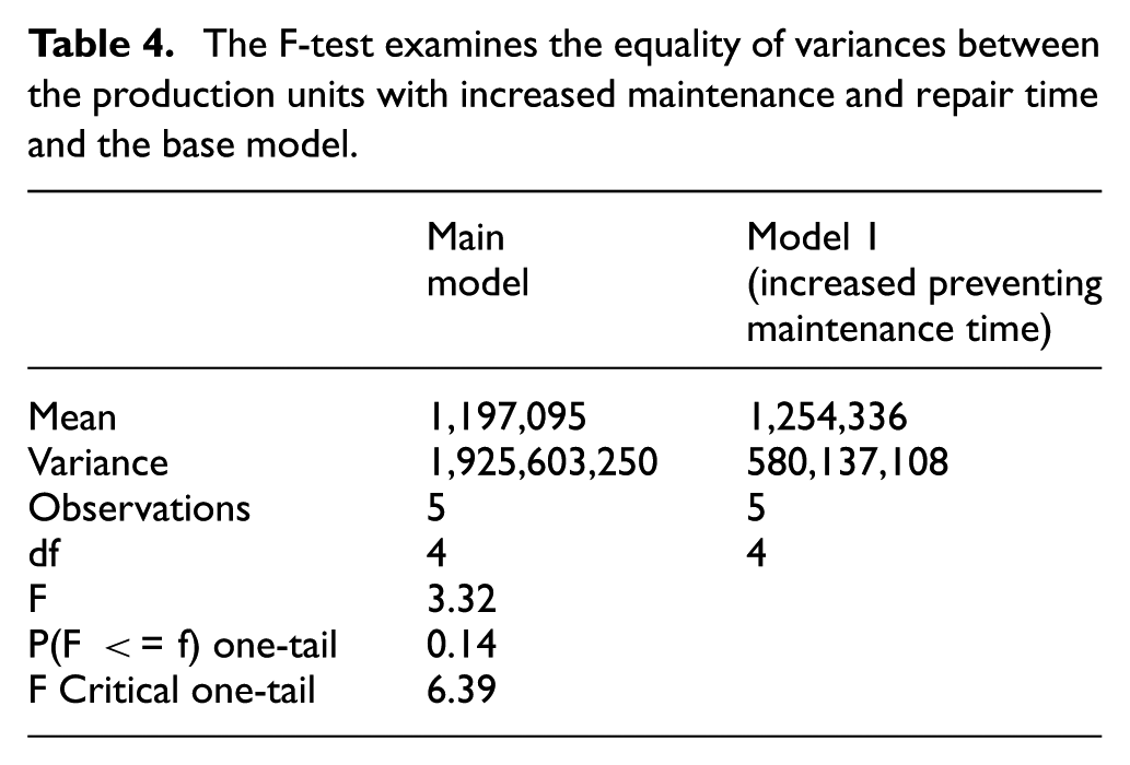
8.4.2. Paired t-test: increased maintenance time

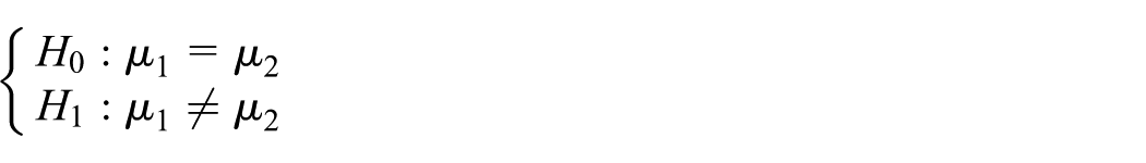
To analyze the effect of increasing maintenance and preventive maintenance time on total costs, a paired t-test was performed. The hypotheses are:

• Null hypothesis (H₀): The averages of the two groups are equal $({\mu }_1={\mu }_2)$ .

• Alternative hypothesis (H₁): The averages of the two groups are not equal $({\mu }_1\ne {\mu }_2)$ .

$$\{\begin{array}{c}{H}_0:{\mu }_1={\mu }_2\hfill \\ \multicolumn{1}{c}{H_1:{\mu }_1\ne {\mu }_2}\end{array}$$

The results are summarized in Table 5, showing a one-tailed P-value of 0.04, which is less than 0.05. Therefore, we reject the null hypothesis and conclude that increasing maintenance time significantly impacts total costs compared to the base model.

Table 5.

Pair of t-tests conducted to analyze the discrepancy in maintenance and repair time between the increased model and the base model.

	Main model	Model 1(increased preventing maintenance time)
Mean	1,197,095	1,254,336
Variance	1,925,603,250	580,137,108
Observations	5	5
Pearson Correlation	−0.17
Hypothesized Mean Difference	0.00
df	4.00
t Stat	−2.39
P(T <= t) one-tail	0.04
t Critical one-tail	2.13

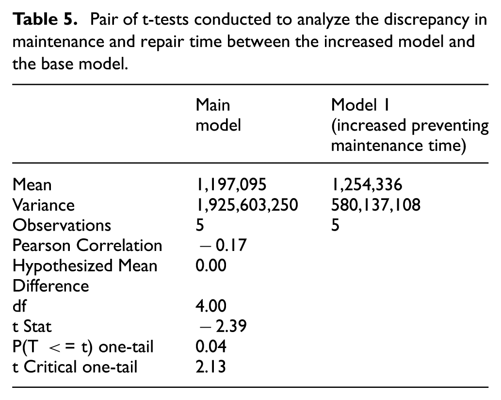
8.4.3. F-test and t-test: increased shortages

Similar analyses were conducted for the scenario where shortages in the final production unit were increased. Table 6 shows the F-test results, where the P-value (0.24) is greater than 0.05, confirming equal variances.

$$\{\begin{array}{c}{H}_0:{\sigma }_1={\sigma }_2\hfill \\ \multicolumn{1}{c}{H_1:{\sigma }_1\ne {\sigma }_2}\end{array}$$

Table 6.

The F-test is used to determine if there is equality of variances between the final production unit and the base model, while allowing for an increase in the allowed shortages.

	Main model	Model 2 (increased backlog)
Mean	1,197,095	1,274,329
Variance	1,925,603,250	4,156,789,161
Observations	5	5
df	4	4
F	0.46
P(F <= f) one-tail	0.24
F Critical one-tail	0.16

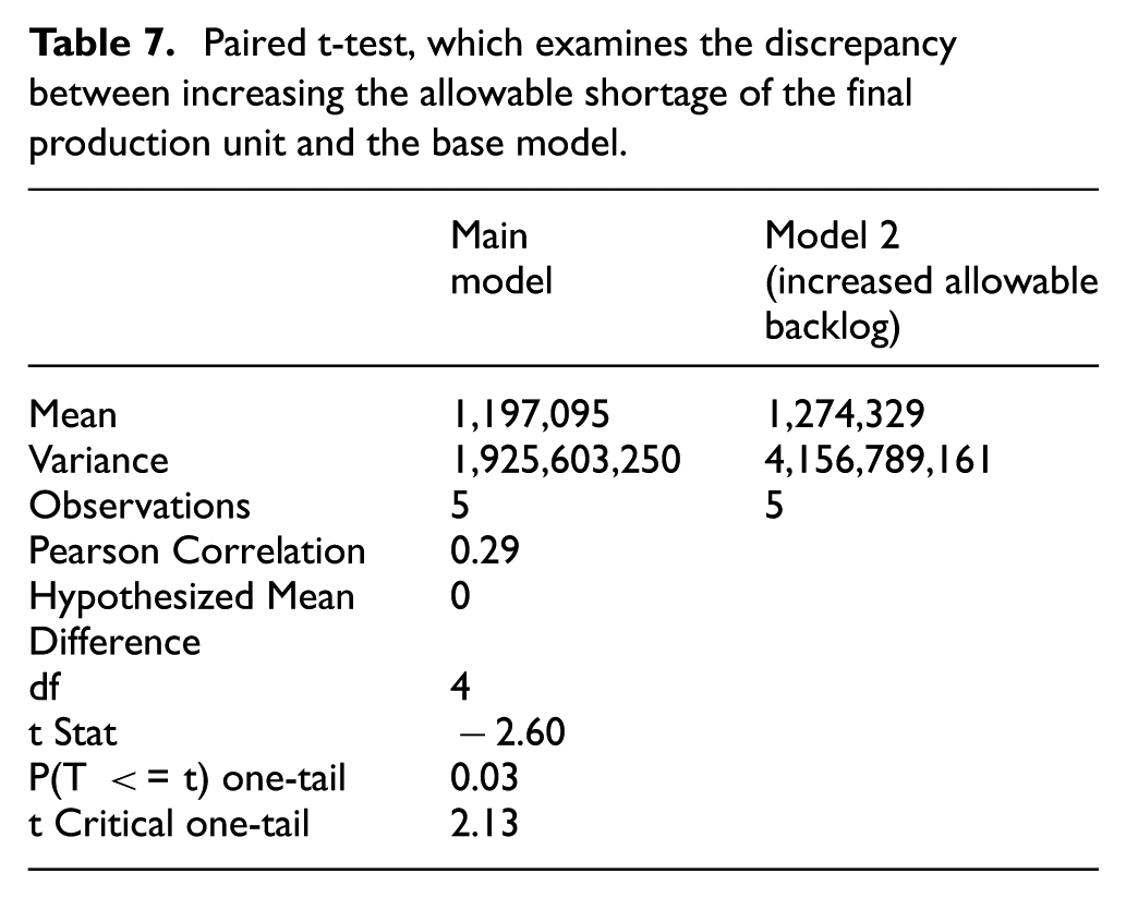
The paired t-test results in Table 7 indicate a significant difference in total costs $(P=0.03)$ . This suggests that allowing for increased shortages significantly affects costs compared to the base model.

Table 7.

Paired t-test, which examines the discrepancy between increasing the allowable shortage of the final production unit and the base model.

	Main model	Model 2(increased allowable backlog)
Mean	1,197,095	1,274,329
Variance	1,925,603,250	4,156,789,161
Observations	5	5
Pearson Correlation	0.29
Hypothesized Mean Difference	0
df	4
t Stat	−2.60
P(T <= t) one-tail	0.03
t Critical one-tail	2.13

8.4.4. F-test and t-test: increased warehouse levels

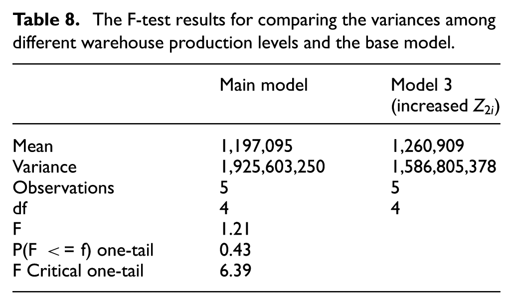
Finally, the impact of increasing warehouse levels on total costs was evaluated. Table 8 confirms equal variances between the base model and the model with increased warehouse levels, as the p-value (0.43) exceeds 0.05.

$$\{\begin{array}{c}{H}_0:{\sigma }_1={\sigma }_2\hfill \\ \multicolumn{1}{c}{H_1:{\sigma }_1\ne {\sigma }_2}\end{array}$$

Table 8.

The F-test results for comparing the variances among different warehouse production levels and the base model.

	Main model	Model 3(increased $Z_{2i}$ )
Mean	1,197,095	1,260,909
Variance	1,925,603,250	1,586,805,378
Observations	5	5
df	4	4
F	1.21
P(F <= f) one-tail	0.43
F Critical one-tail	6.39

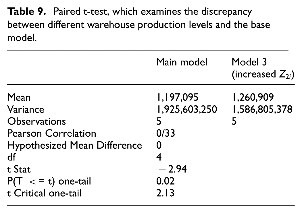
The paired t-test results in Table 9 show a p-value of 0.02, indicating a statistically significant difference in costs. Therefore, increasing warehouse levels also has a notable impact on total costs compared to the base model.

$$\{\begin{array}{c}{H}_0:{\mu }_1={\mu }_2\hfill \\ \multicolumn{1}{c}{H_1:{\mu }_1\ne {\mu }_2}\end{array}$$

Table 9.

Paired t-test, which examines the discrepancy between different warehouse production levels and the base model.

	Main model	Model 3(increased $Z_{2i}$ )
Mean	1,197,095	1,260,909
Variance	1,925,603,250	1,586,805,378
Observations	5	5
Pearson Correlation	0/33
Hypothesized Mean Difference	0
df	4
t Stat	−2.94
P(T <= t) one-tail	0.02
t Critical one-tail	2.13

These results validate the proposed model’s ability to evaluate the cost implications of adjustments to maintenance, shortages, and inventory levels effectively.

9. Case study

The production system is susceptible to failure in an ambiguous network consisting of four production units as shown in Figure 15.

Figure 15.

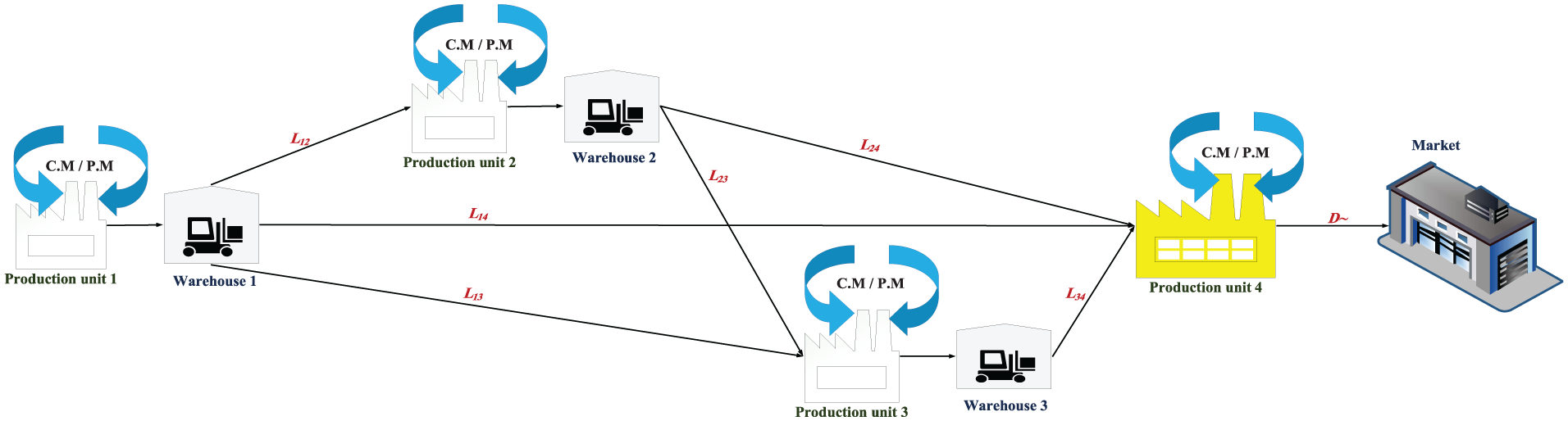
Failure-prone manufacturing system with 4 production unit.

This is done in order to ascertain the optimal production rate and timing for preventive maintenance and repair. The potential demand for final items is measured in units of items per unit of time, and the maximum production rate per unit of production is set according to the following criteria. It should be noted that the production rates are determined using the relationships outlined in equations (5) and (6).

• When the demand for the final product is equal to 1 unit of items per unit of time, the production rate for the first to third production units (in units of items per unit of time) is determined as follows:

$$u_1^{\max }=180,u_2^{\max }=60,u_3^{\max }=20,u_4^{\max }=5$$

• The production rate of the first to third production units (units of items per unit of time) is determined as follows if the demand for the final product is equal to 3 units of items per unit of time:

$$u_1^{\max }=270,u_2^{\max }=84,u_3^{\max }=26,u_4^{\max }=8$$

• The production rate of the first to third production units (measured in units of items per unit of time) is determined based on the demand for the final product, which is equal to 6 units per unit of time.

$$u_1^{\max }=360,u_2^{\max }=108,u_3^{\max }=32,u_4^{\max }=11$$

• If the demand for the final product is 10 units of items per unit of time, the production rate of the first three production units (measured in units of items per unit of time) is determined as follows:

$$u_1^{\max }=480,u_2^{\max }=140,u_3^{\max }=40,u_4^{\max }=15$$

The maximum number of passport requests is k = 10 (units of items).

The consumption coefficients are defined as $l_{12}=3,l_{13}=3,l_{14}=4,l_{23}=7,l_{24}=5$ and $l_{34}=1$

This means that to produce one unit of product on Machine 4 (final product), 4 units of the product from Machine 1 $(l_{14}=4)$ , 5 units of the product from Machine 2 $(l_{24}=5)$ , and 1 unit of the product from Machine 3 $(l_{34}=1),$ are required. Similarly, to produce one unit of product on Machine 3, 3 units of the product from Machine 1 $(l_{13}=3),$ and 7 units of the product from Machine 2 $(l_{23}=7)$ , are required. To produce one unit of product on Machine 2, 3 units of the product from Machine 1 $(l_{12}=3)$ are utilized. In addition, it is assumed that at the initial time of the simulation, the inventories of Machines 1, 2, and 3 have initial stock, while the inventory of Machine 4 is empty. Accordingly, the initial inventory levels for each product are defined as follows:

$$(x_1=70,x_2=50,x_3=5,x_4=0)$$

The capacity of each warehouse (z₂) is also taken into consideration in the following manner:

$$(Z_{21}=3000,Z_{22}=500,Z_{23}=300,Z_{24}=15)$$

The average duration of maintenance and preventive repairs of the production unit is calculated using the exponential distribution with parameters ${\mu }_3=25,{\mu }_2=20,{\mu }_1=15$ and ${\mu }_4=30$ (in time unit), This optimization of the decision variable is crucial for achieving the objectives of the problem. We also consider the average maintenance and repair time, represented by ${\lambda }_3=40,{\lambda }_2=30,{\lambda }_1=25$ and ${\lambda }_4=60$ (in time unit).

The cost of holding each product in the warehouse is $h_3=20,h_2=15,h_1=10$ and $h_4=25$ per unit time. It has been observed that the cost of storing items increases due to the increase in value added.

The cost of storing items has been observed to increase due to the increase in value added. In addition, if items remain in storage for 90 days, they become unusable. The cost of shortage of fuel per unit of items is $C_p=60$ . The cost of Perishable per unit of items is measured in units of money. The cost of lost sales per unit of items is $\hat{\ell }=90$ units of money. The cost of a lost sales deficit, which occurs when the organization’s credit is deducted, is higher than the cost of a deficit. Furthermore, the cost of producing each unit of product $i$ per unit of time is $c_1=10,c_2=20,c_3=30$ , and $c_4=40$ . The production of defective items is influenced by the age of the production unit. As the life of the production unit increases, the likelihood of producing a defective product also increases. However, preventive maintenance and repairs can reset the age of the production unit back to zero, reducing the chances of defect production.

A control point, referred to as, is defined to determine the optimal timing for preventive maintenance and repairs. When the inventory level reaches this point, preventive maintenance and repairs will be production unit out.

The simulation lasts for 365 working days of 8 h. To determine the number of repetitions for each scenario, we use the equations (34)–(39). Assuming a relative confidence interval of 23% and a probability of committing the first type error of 0.05 $(\mathrm{\alpha }=0.05)$ , the minimum required repetitions are 5. This means that each scenario will be repeated 5 times. In this particular example, the coefficient of change is estimated to be approximately 12% based on the number of repetitions. It is important to note that the line balance is taken into consideration when determining the system parameters in the above numerical example.

The simulation of this system utilizes 5 independent and distributed IIDs to execute each scenario in the model. This requires initializing both the system and the statistics. Each iteration begins with an empty system at zero time and ends after 365 days. The use of a random number generator ensures that the values generated are independent and distributed across iterations. This information is included in the model, and the simulation is then initiated using the Arena software. Following the simulation, an analysis of the inventory level and production rate charts, as well as an analysis of the system costs, will be conducted.

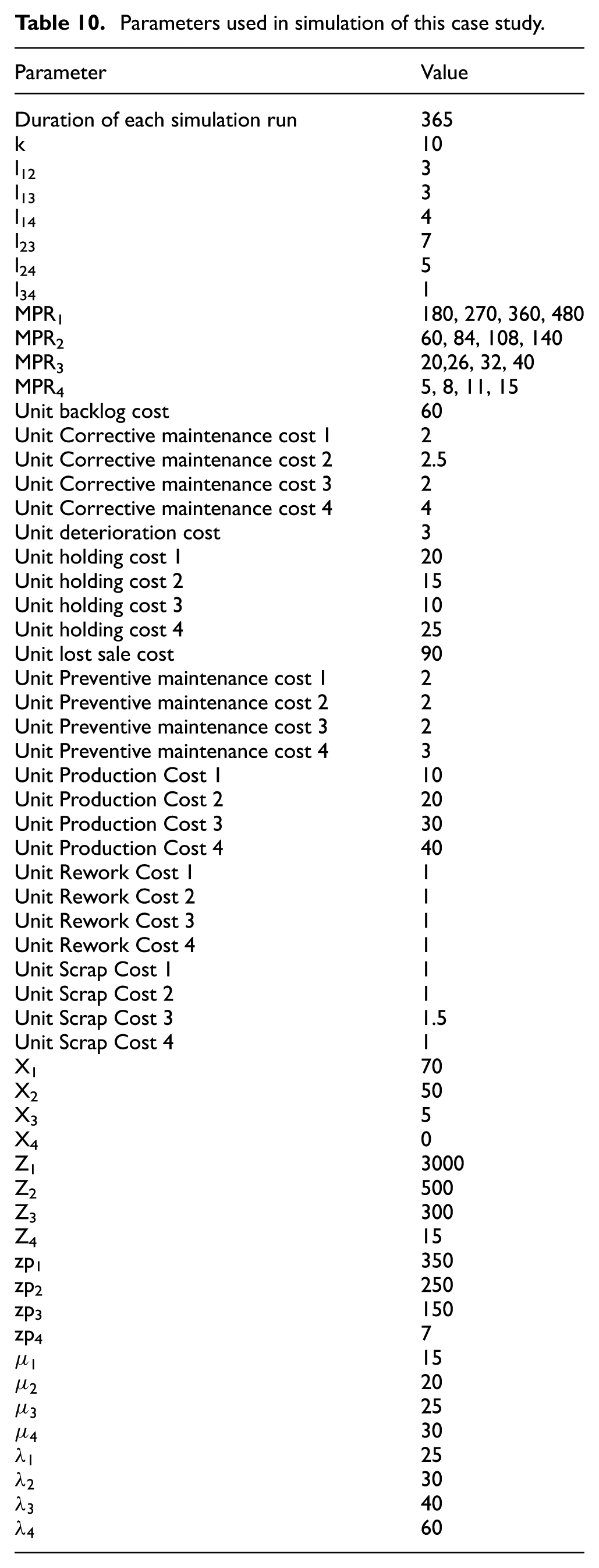
The parameters utilized in simulation of case study is shown in Table 10:

Table 10.

Parameters used in simulation of this case study.

Parameter	Value
Duration of each simulation run	365
k	10
l12	3
l13	3
l14	4
l23	7
l24	5
l34	1
MPR1	180, 270, 360, 480
MPR2	60, 84, 108, 140
MPR3	20,26, 32, 40
MPR4	5, 8, 11, 15
Unit backlog cost	60
Unit Corrective maintenance cost 1	2
Unit Corrective maintenance cost 2	2.5
Unit Corrective maintenance cost 3	2
Unit Corrective maintenance cost 4	4
Unit deterioration cost	3
Unit holding cost 1	20
Unit holding cost 2	15
Unit holding cost 3	10
Unit holding cost 4	25
Unit lost sale cost	90
Unit Preventive maintenance cost 1	2
Unit Preventive maintenance cost 2	2
Unit Preventive maintenance cost 3	2
Unit Preventive maintenance cost 4	3
Unit Production Cost 1	10
Unit Production Cost 2	20
Unit Production Cost 3	30
Unit Production Cost 4	40
Unit Rework Cost 1	1
Unit Rework Cost 2	1
Unit Rework Cost 3	1
Unit Rework Cost 4	1
Unit Scrap Cost 1	1
Unit Scrap Cost 2	1
Unit Scrap Cost 3	1.5
Unit Scrap Cost 4	1
X1	70
X2	50
X3	5
X4	0
Z1	3000
Z2	500
Z3	300
Z4	15
zp1	350
zp2	250
zp3	150
zp4	7
${\mu }_1$	15
${\mu }_2$	20
${\mu }_3$	25
${\mu }_4$	30
${\lambda }_1$	25
${\lambda }_2$	30
${\lambda }_3$	40
${\lambda }_4$	60

9.1. Replications and duration of simulation

To perform analysis on the model outputs, it is important to determine the appropriate number of replications and the duration of execution. The number of simulation iterations can be determined using a coefficient index of changes, which indicates the ratio of the standard deviation to the mean of the data. The coefficient of change can be calculated using the following equation:

$$C.V=\frac{\sigma }{\mu }$$

(34)

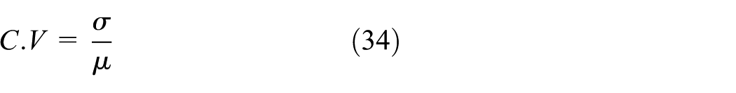
We use the following estimator to estimate the coefficient of change.

$$C.V=\frac{S}{\overline{X}}=\frac{\sqrt{\sum _{i=1}^n{(x_i-{\overline{X}}_i)}^2/(n-1)}}{\sum _{i=1}^n{x}_i/n}$$

(35)

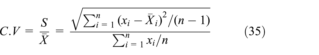
In this case, X represents the average total cost of the system per unit of time per simulation. Meanwhile, n denotes the number of performances. The estimated cost of the system can be determined by considering the distance.

$$\overline{X}\pm t_{\frac{\alpha }{2};n-1}\frac{S}{\sqrt{n}}$$

(36)

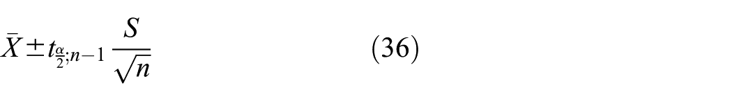
As n increases, the distance estimate becomes shorter and approaches the point estimate. To reduce the length of the distance estimate from a specific value, l, the number of simulation runs is determined. In order to achieve this, the following relationships are utilized:

$$2t_{\frac{\alpha }{2};n-1}\frac{S}{\sqrt{n}}\le l$$

(37)

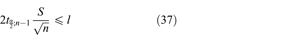
The length of the distance estimation, l, is measured by dividing the parties in the relationship and calculating the ratio of the mean data.

$$2t_{\frac{\alpha }{2};n-1}\frac{S}{\overline{X}\sqrt{n}}\le \frac{l}{\overline{X}}$$

(38)

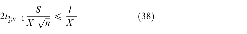
IF $\frac{l}{\overline{X}}=L$ , we will have:

$$n\ge {\left[2t_{\frac{\alpha }{2};n-1}\frac{C.V}{L}\right]}^2$$

(39)

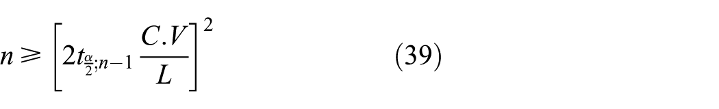
Therefore, in order to establish the relationship mentioned above, ¹ the value of n must be selected accordingly. If the relative confidence interval is 23% and the probability of committing a type I error, α, is 0.05, a minimum of 5 repetitions is required. This means that each scenario should be repeated 5 times. In this particular example, the coefficient of change is estimated to be approximately 12% based on the number of repetitions. It is important to note that in the numerical example provided, the line balance is taken into consideration when determining the system parameters. Furthermore, the simulation of this system utilizes 5 independent and identically distributed (IIDs) scenarios, initializing both the system and the statistics. As a result, each iteration begins with an empty system at time zero and concludes after 365 days. The use of a random number generator ensures that the generated values are independent and distributed throughout the iterations.

9.2. Analysis of the inventory level and production rate of intermediate production units

In this section of the article, we will analyze the charts of the inventory level and the production rate based on the level of control defined for the intermediate production units in equation (18). As mentioned earlier, the simulation executes each scenario using independent and distributed iterations. This means that the system and statistics are initialized in each iteration, causing the simulation to start at zero time and end after 365 days. Figures 16 and 17 depict the graph of the inventory level and the graph of the production rate specifically for the first production unit.

Figure 16.

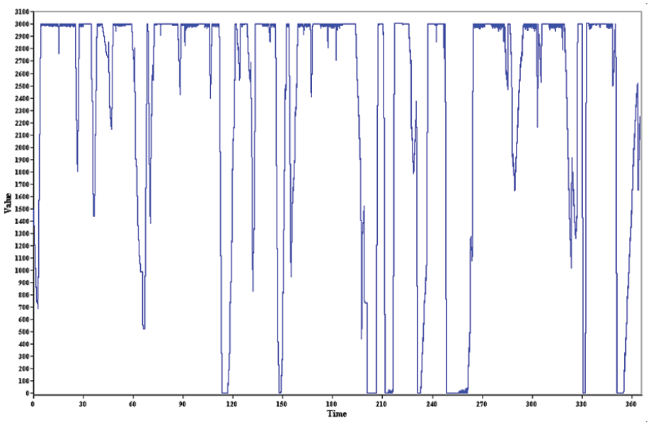
Chart of the inventory level of the production unit 1.

Figure 17.

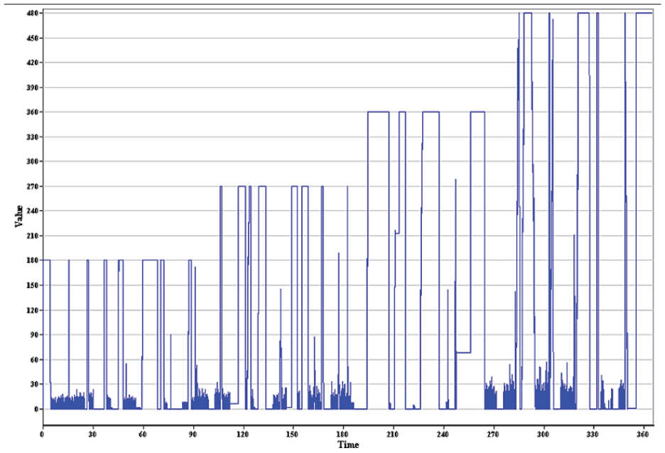
Chart of the production rate of the production unit 1.

As illustrated in Figure 17, the system follows a specific control policy (equation (18)) to ensure that production continues until the inventory level reaches the warehouse threshold. Once the inventory reaches this threshold, production stops and the required number of units for production is supplied from the warehouse. This leads to a decrease in the warehouse inventory level. During this time, the production rate is zero due to a production unit failure. At the 10th moment, the warehouse inventory reaches zero and the production unit starts producing at its maximum capacity to meet the demand of the next production units, preventing any disruption in the production process. Moments like the range of 30-10 show that even though the warehouse inventory level is not zero, the production unit operates at its maximum power due to a production unit failure. This leads to a decrease in warehouse inventory and once the production unit is back in operation, the inventory level increases again. The inventory level of this particular production unit fluctuates between 0 and 3000, ensuring that it never faces shortages, which is an important assumption of the problem. The production rate of the first production unit varies and increases during times when the inventory is zero, as indicated in the production rate chart.

Figures 18 and 19 depict the inventory level and production rate of the second production unit at any given moment.

Figure 18.

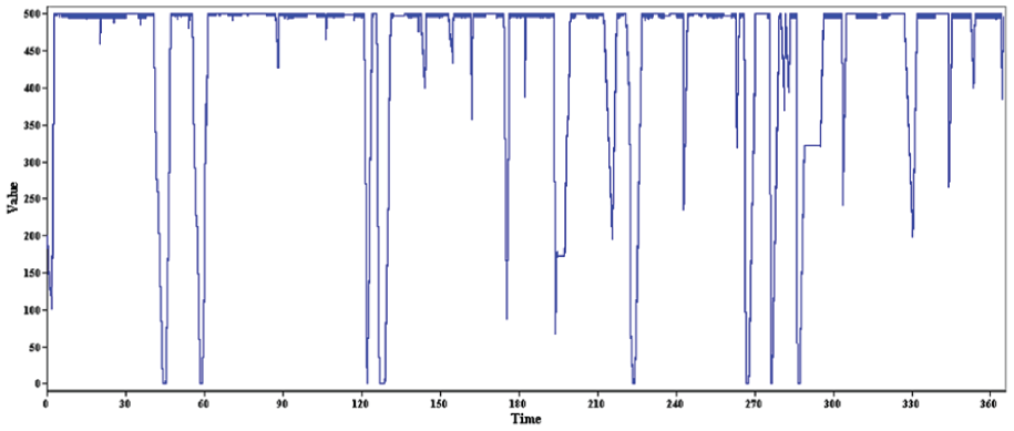
Chart of the inventory level of the production unit 2.

Figure 19.

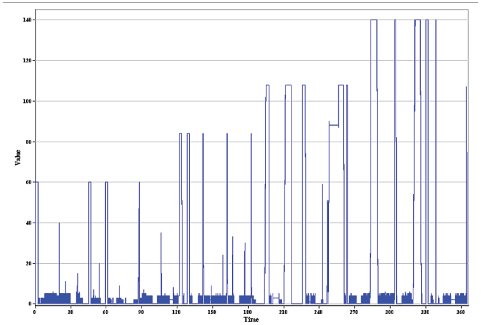
Chart of the production rate of the production unit 2.

As shown, the production rate of the second unit also fluctuates between zero and the warehouse level of 235, ensuring it does not experience shortages. At the moment of 100-50, the warehouse inventory level reaches zero, prompting the production unit to operate at maximum capacity. Prior to this, the production unit had already started operating at maximum power, indicating that the relationship had been established. For instance, at the 100th moment, a production unit failure occurred and the production rate dropped to zero, resulting in a decrease in warehouse inventory. Once the production unit is repaired and resumes production, the inventory level increases again.

Figures 20 and 21 depict the inventory level and production rate of the third production unit.

Figure 20.

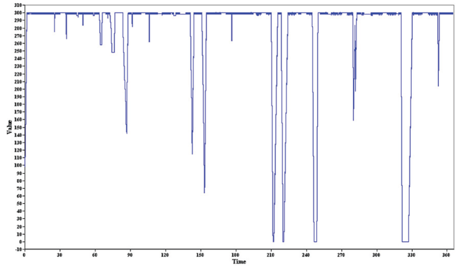
Chart of the inventory level of the production unit 3.

Figure 21.

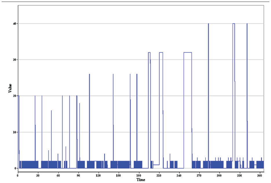
Chart of the production rate of the production unit 3.

The analysis of this unit is identical to that of the first and second units. The production rate in this unit can range from zero to 500, but should not exceed this limit. Similar to the previous units, unauthorized shortages are observed in this unit, with inventory levels fluctuating between zero and the third warehouse level of 300. Once the inventory level reaches the warehouse level, production ceases and the production rate drop to zero. From time 200 to 150, a failure in the production unit occurs, leading to a decrease in inventory levels. Following repairs, production resumes.

9.3. Analysis inventory level and production rate of the final production unit

Figures 22 and 23 depict the inventory level and production rate of the final production unit.

Figure 22.

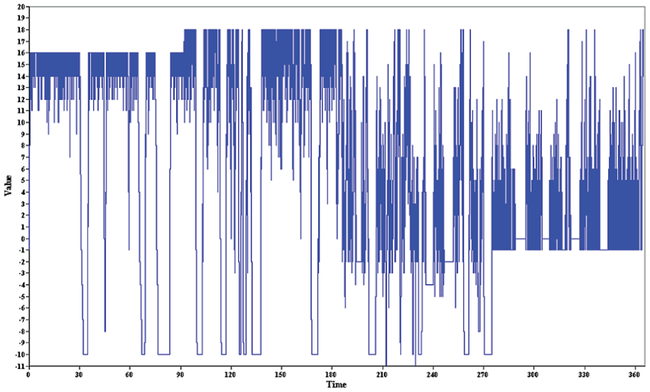
Chart of the inventory level of the production unit 4.

Figure 23.

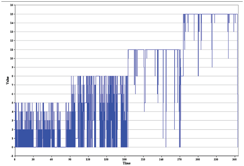
Chart of the production rate of the production unit 4.

As stated in the hypotheses presented in the first and third chapters, shortages are allowed in this production unit. The control level of the unit follows relationship (19). Figure 23 confirms the hypothesis of shortages, as the inventory fluctuates between the permissible shortage rate (10-) and the warehouse level of 35. In addition, there is a Perishable of items in this production unit, which further reduces the inventory level in the warehouse. When the production unit reaches 0-50, it is unable to produce, leading to a production rate of zero. Consequently, demand is fulfilled from the warehouse inventory, causing a decrease in its level until the system encounters a shortage of 10 units of items.

9.4. Simulation optimization

After simulating the system, as discussed in the previous section, the system optimization is performed using the Scatter Plot tool. Arena is a widely recognized and powerful discrete simulation software globally. It offers various capabilities and tools that enable analysts to analyze data and model outputs at each stage of the simulation implementation. One of these tools is the Scatter Plot tool. This tool helps identify the best scenario among thousands of specified scenarios based on constraints and the target function. Within this tool, multiple objective functions of maximization and minimization types can be defined. Tabu Search and Scatter Search algorithms are utilized by this tool to identify the optimal scenario. The purpose of utilizing this tool is to determine the most suitable scenario for minimizing total production costs, maintenance costs, items Perishable, scrap, rework, as well as corrective and preventive maintenance and repairs.

Once decision variables are defined as control variables, which include optimal shortages, optimal capacity of first to fourth machine warehouses, time required for implementing preventive maintenance and repairs for machines, as well as specific inventory for preventive maintenance and repairs, and target functions are established, the search for the optimal solution commences. As shown in Figure 24 the model implementation results reveal that the best scenario was selected after 400th iterations, and no further changes occurred, indicating that the model reached a stable state.

Figure 24.

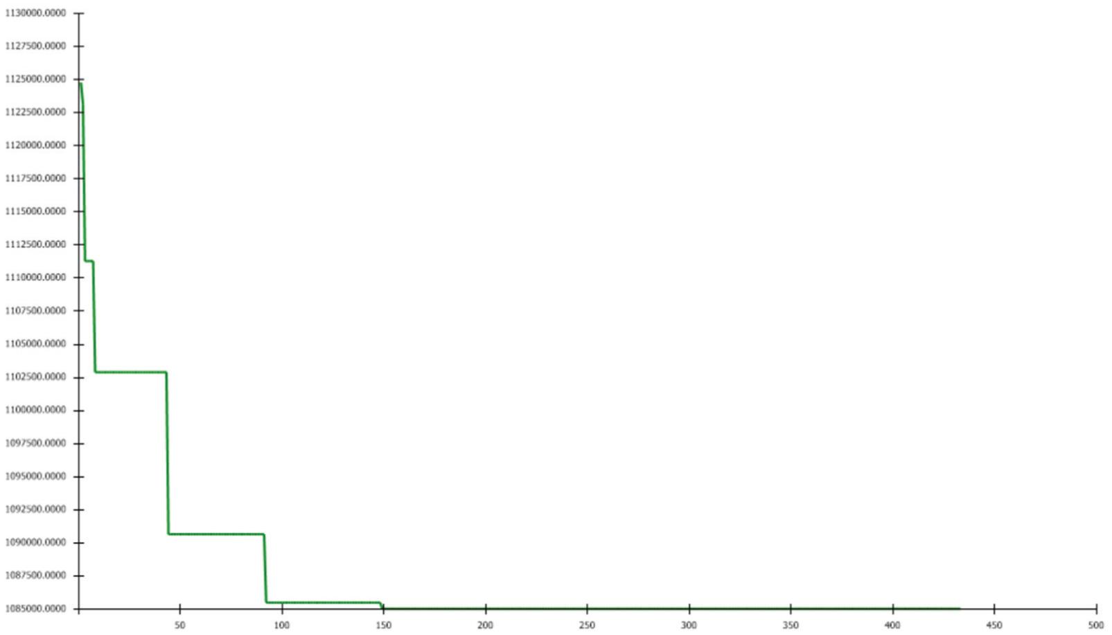
Chart on the total cost optimization.

The results are presented in the Table 11:

Table 11.

Optimization of decision variables in FPMS with 4 production units.

Control name	First value	Best value
K	10	10
Time of PM1	15	13
Time of PM2	20	18
Time of PM3	25	24
Time of PM4	32	32
Z21	825	795
Z22	235	219
Z23	25	23
Z24	30	27
Zp1	450	400
Zp2	110	98
Zp3	15	14
Zp4	10	10
Total cost	1,125,000	1,080,000

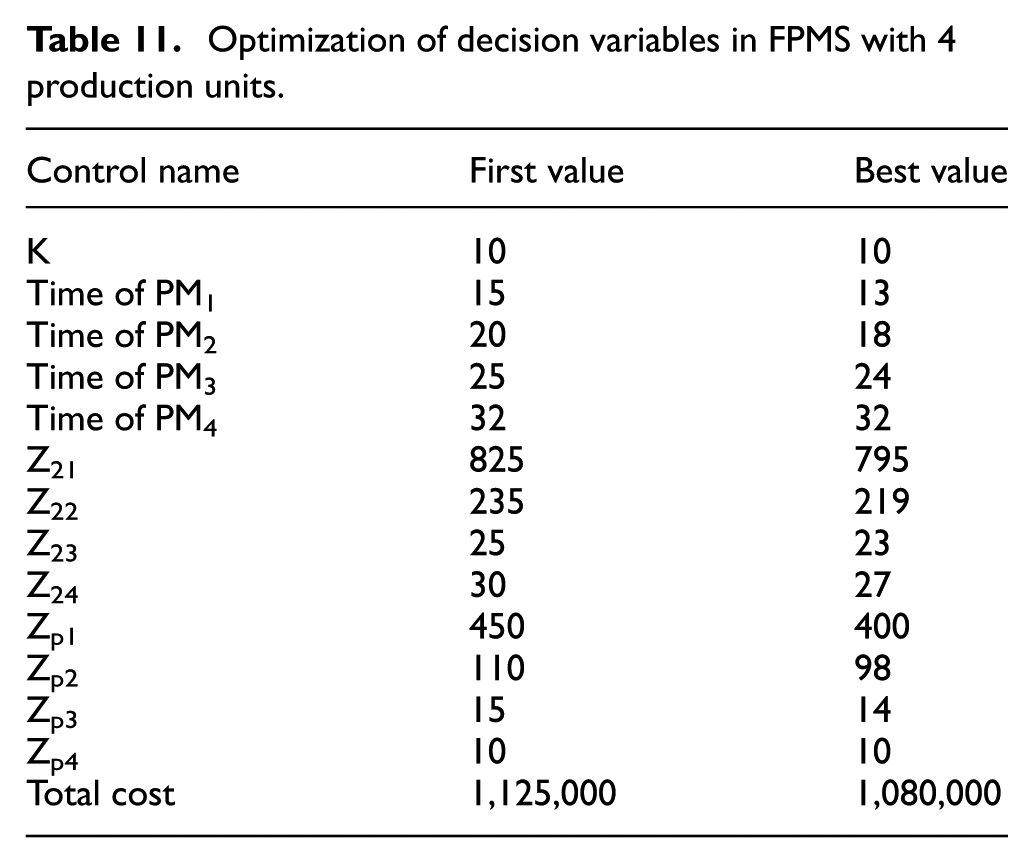
The table below displays the optimal values of the decision variables corresponding to the graph above. These values have increased from 1,125,000 monetary units to 1,080,000 in the 400 m repeat by incorporating these variables into the cost model.

9.5. Optimization model with Tabu search algorithm

The simulation of the Tabu search algorithm in the Arna software is shown in Figure 25.

Figure 25.

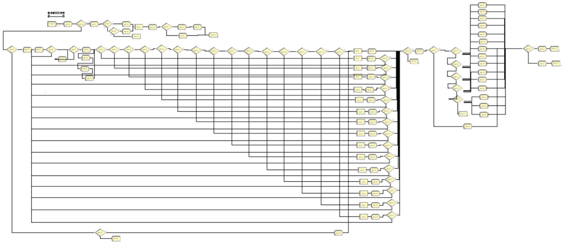
Simulation of the Tabu search algorithm in the Arna software.

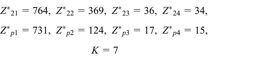
In this problem, the neighborhood radius for decision variables is defined as: the neighborhood radius of the threshold level of the first and second production unit storage $[Z_{2i}\pm 20]$ , the neighborhood radius of the threshold level of the third and fourth production unit storage $[Z_{2i}\pm 3]$ , the neighborhood radius of the number of deficiencies in the form of $[K\pm 1]$ , the neighborhood radius of the inventory minimum in order to production unis out preventive maintenance and repairs for the first and second production units in the form of $[Z_{\mathrm{pi}}\pm 20]$ and for the third and fourth production units in the form of $[Z_{\mathrm{pi}}\pm 3]$ is considered. This is because decision variables are meaningful at these intervals. In the meta-heuristic algorithm, if the neighborhood radius is chosen too small, we may be late to the optimal answer; as well as by choosing the large neighborhood radius, we may be far from the optimal answer. For this reason, the choice of the excavation area is of great importance. In this article, by analyzing the sensitivity on the neighboring radius, the area of exploration is considered as mentioned. The Tabu list is a multi-array variable with 15 rows and 13 columns, with the number 15 indicating the length of the list and the number 13 indicating the number of decision variables examined in this article.

The algorithm’s stop condition can be determined by stopping the algorithm if the target function reaches the predefined threshold value. So, the condition for stopping the algorithm in this study is that if the average total cost is reduced by more than 4%, the algorithm is stopped.

With the complete implementation of the algorithm, it is observed that in the 19th iteration (iteration of 95 to 100 simulation models), the average total cost decreases from 1,125,000 monetary units to 1,078,502 monetary units, which has decreased by more than the expected value, i.e., about 5%, and the algorithm stops in this iteration.

$$\begin{array}{c}{Z^{*}}_{21}=764,{Z^{*}}_{22}=369,{Z^{*}}_{23}=36,{Z^{*}}_{24}=34,\hfill \\ {Z^{*}}_{p1}=731,{Z^{*}}_{p2}=124,{Z^{*}}_{p3}=17,{Z^{*}}_{p4}=15,\hfill \\ K=7\hfill \end{array}$$

When comparing the results of the two optimization methods, it is worth noting that the Tabu search meta-heuristic algorithm, implemented in the arena software.

$$\begin{array}{c}\multicolumn{1}{c}{u_{i=1}(t)=\{\begin{array}{c}0x_i(t)>z_{2i}\hfill \\ \multicolumn{1}{c}{u_i^{\max }{x}_i\left(t\right)+u_i^{\max }<z_{2i}}\\ \multicolumn{1}{c}{[z_{2i}-x_i(t)]\mathrm{Otherwise}}\end{array}}\\ \multicolumn{1}{c}{u_{i=2}(t)=\{\begin{array}{c}0x_i(t)>z_{2i}\hfill \\ \multicolumn{1}{c}{u_i^{\max }{x}_i\left(t\right)+u_i^{\max }<z_{2i}}\\ \multicolumn{1}{c}{[z_{2i}-x_i(t)]\mathrm{Otherwise}}\end{array}}\\ \multicolumn{1}{c}{u_{i=3}(t)=\{\begin{array}{c}0x_i(t)>z_{2i}\hfill \\ \multicolumn{1}{c}{u_i^{\max }{x}_i\left(t\right)+u_i^{\max }<z_{2i}}\\ \multicolumn{1}{c}{[z_{2i}-x_i(t)]\mathrm{Otherwise}}\end{array}}\\ u_{i=4}(t)=\{\begin{array}{c}0x_i-d>z_{2i}\hfill \\ \multicolumn{1}{c}{u_i^{\max }{x}_i+u_i^{\max }+u_{\mathrm{rem}}^{\max }-d<z_{2i}}\\ \multicolumn{1}{c}{z_{2i}-(x_i-d)\mathrm{Otherwise}}\end{array}\hfill \end{array}$$

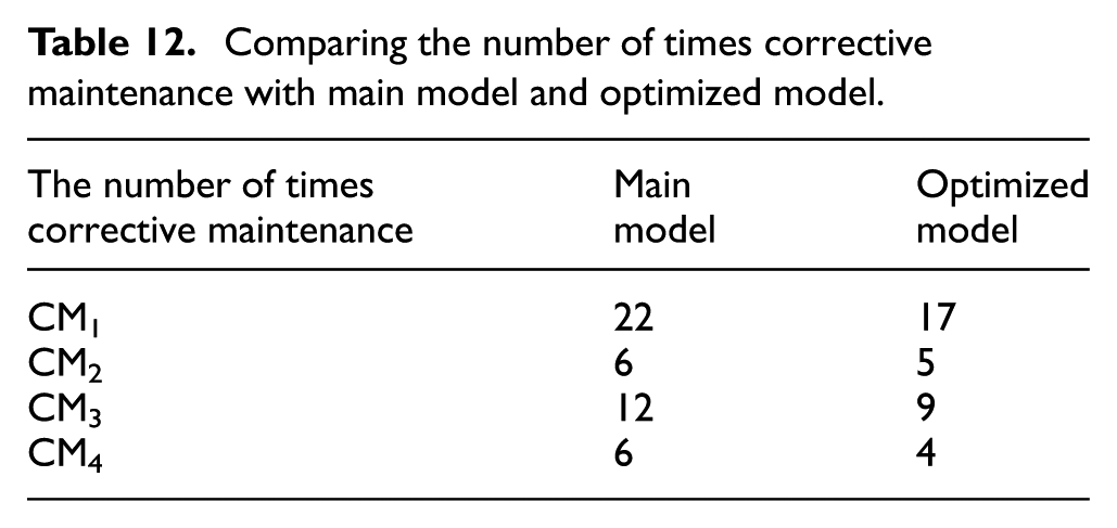
As shown in Table 12 and Figure 26, the reduction in intervals between preventive maintenance has significantly decreased the occurrence of unforeseen failures. This helps prevent system downtime, potential shortages, and loss of organizational credibility. This reduction serves as a clear indication of the model’s effectiveness.

Table 12.

Comparing the number of times corrective maintenance with main model and optimized model.

The number of times corrective maintenance	Main model	Optimized model
CM1	22	17
CM2	6	5
CM3	12	9
CM4	6	4

Figure 26.

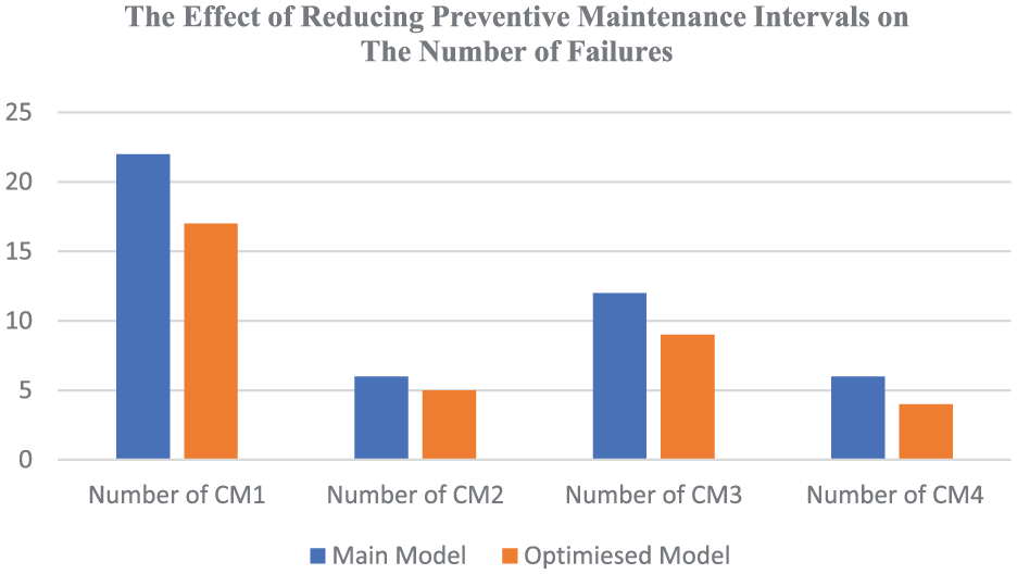
The effect of reducing preventive maintenance intervals on the number of failures.

In order to demonstrate the effectiveness of the model presented, we utilized the optimal solution from the previous problem involving 4 production units to model a problem with 6 production units as Figure 27.

Figure 27.

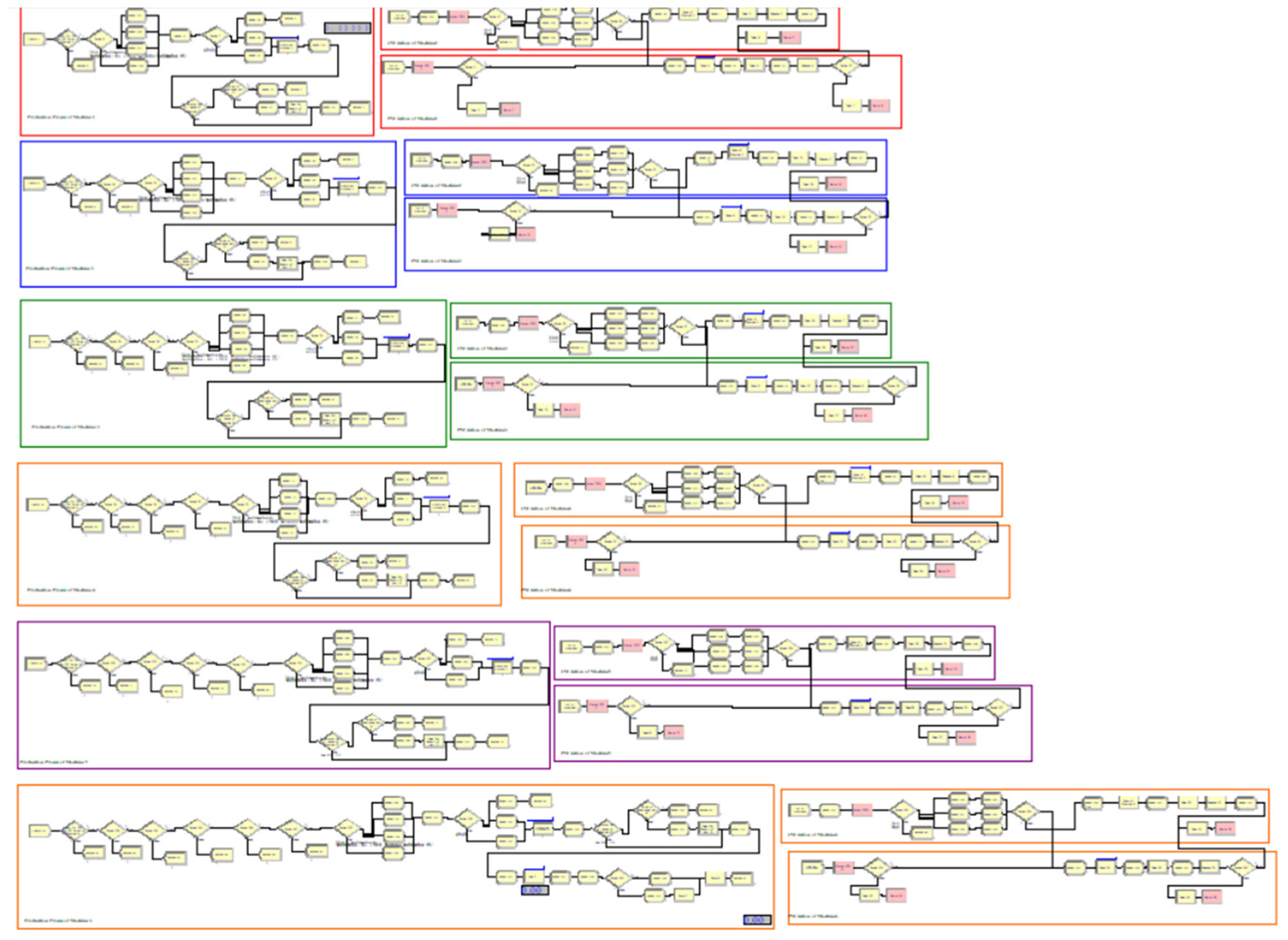
Simulation of manufacturing system with 6 production units.

The optimal solutions were then calculated in the same manner as before. Similarly, we used the optimal solution from the problem with 6 production units to tackle the larger problem involving 10 production units. By examining the results obtained from these analyses, it has been determined that this model is capable of addressing complex problems, even when incorporating additional assumptions that closely resemble real-world scenarios.

The optimal solutions of the problem with 6 production units and using the Tabu search algorithm coded in the ARENA.14 software is shown in Table 13.

Table 13.

Optimization of decision variables in FPMS with 6 production units.

Control name	First value	Best value
K	10	11
Time of PM1	13	9
Time of PM2	18	15
Time of PM3	24	20
Time of PM4	32	30
Time of PM5	45	38
Time of PM6	30	20
Z21	795	824
Z22	219	226
Z23	23	20
Z24	27	29
Z25	25	28
Z26	25	30
Zp1	400	415
Zp2	98	114
Zp3	14	10
Zp4	10	15
Zp5	20	23
Zp6	12	15
Total cost	2,358,400	2,249,000

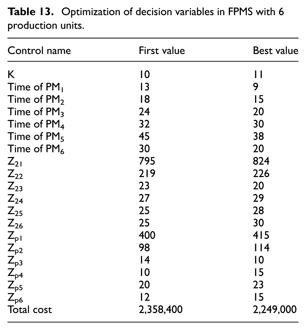
Finally, the simulation was conducted on a failure-prone Manufacturing system of large size, consisting of 10 production units. The results of the simulations for the small-sized system (4 production units) and the medium-sized system (6 production units) were then analyzed in the same manner. The investigation results demonstrate that in this system, the total cost has decreased from 5974000 to 5256000. This indicates the model’s efficiency in handling large problems.

9.6. Description with inputs, effectiveness metrics, and RCM-risk integration

In order to evaluate the effectiveness of the production system under different maintenance and operational scenarios, a set of Key Performance Indicators (KPIs) have been used. These quantitative metrics provide a basis for comparing system performance and assessing the impact of maintenance strategies and production planning decisions. In order to enhance the clarity and reproducibility of the case study, this section as Table 14 presents the key performance metrics used to evaluate the system, and the adopted maintenance strategy, including RCM and risk analysis.

Table 14.

Key performance indicators (KPIs) for evaluating production system effectiveness.

KPI	Description	Unit	Relevance to study
Total System Cost	Total cost including production, maintenance, inventory, shortage, and waste	Currency units (e.g., $)	Primary objective function for optimization
Availability	Ratio of uptime to total time for each production unit	%	Reflects equipment reliability and maintenance effectiveness
Average Inventory Level	Mean stock level for each product throughout the simulation	Units	Indicates storage efficiency and related costs
Mean Time to Failure (MTTF)	Average time between failures for each production unit	Time units (e.g., hours)	Measures equipment reliability
Number of Defective Items	Total number of products failing quality requirements	Units	Represents production quality and maintenance impact
Service Level	Ratio of demand fulfilled to total demand	%	Reflects the ability to meet customer demand and minimize shortages

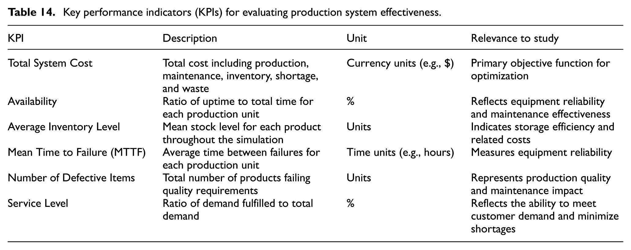
The main KPIs considered in this study are as follows:

• Total System Cost: The aggregate of maintenance costs, production costs, inventory holding costs, shortage penalties, and cost of defective items. This metric is the primary objective in the optimization model.

• Availability: The proportion of time each production unit is in an operational (non-failed) state relative to the total simulation time. This measures the effectiveness of maintenance planning.

• Average Inventory Level: The mean inventory level across all products over the simulation period. It indicates the logistical efficiency and storage cost implications.

• Mean Time to Failure (MTTF): The average time between two consecutive failures of each production unit, reflecting the reliability of the equipment.

• Number of Defective Items: The total number of defective products generated during the simulation. This serves as a quality control metric and is impacted by equipment age and maintenance frequency.

• Service Level: The ratio of fulfilled demand to total demand, indicating the system’s ability to meet customer requirements.

These metrics were selected because they directly reflect the operational, economic, and reliability aspects of the system, and are commonly used in production and maintenance optimization studies.

Availability is calculated by dividing the total operational time of each production unit by the sum of its operational and downtime periods. The formula used is:

$$\mathrm{Availability}=\frac{\mathrm{Uptime}}{\mathrm{Uptime}+\mathrm{Downtime}}$$

These values are extracted from the simulation logs, which monitor the status of each machine over the 365 working days.

The plant currently uses a time-based preventive maintenance strategy, which was modeled in the simulation using exponential failure and repair distributions. To improve maintenance decision-making, a Reliability-Centered Maintenance (RCM) approach was implemented:

• RCM Analysis: Functional failures were identified for each unit, and a Failure Mode and Effects Analysis (FMEA) was conducted to prioritize components using Risk Priority Numbers (RPN = Severity × Occurrence × Detectability).

• Risk Assessment: A risk matrix was used to quantify operational risk, based on the probability of failure, the severity of its impact on production and cost, and detection time.

• High-risk components (e.g., units with high failure frequency and cost impact) were selected for targeted preventive maintenance planning.

This structured approach ensures a comprehensive evaluation of the system’s performance and the effectiveness of maintenance policies.

Table 15, presents a comparative risk analysis of the production units before and after the implementation of RCM.

Table 15.

Risk analysis of production units before and after RCM implementation.

Component	Probability of failure (λ)	Severity (cost impact per failure)	Risk (λ× cost)	RCM action	Residual risk (after RCM)	Risk reduction (%)
Unit 1	0.04	400	16	PM every 13 days	6	62.5%
Unit 2	0.05	600	30	PM every 18 days	10	66.7%
Unit 3	0.07	800	56	PM every 24 days	18	67.9%
Unit 4	0.06	1000	60	PM every 32 days	20	66.7%

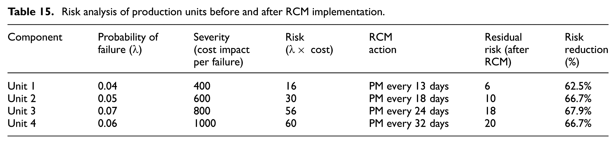
As shown, the preventive and predictive maintenance strategies significantly reduced the risk level, with an average reduction of over 65%. This improvement justifies the cost and complexity of applying the RCM framework to the current system.

10. Conclusion

This research focuses on studying a network failure-prone system (NFPMS) that produces multiple products. The system assumes that the products are unstable. Each stage of production relies on the product from the previous stage, with a specific consumption factor. The machines may fail during production but are repaired and return to the production process. In the final stage of the system, shortages of backlog and lost sales are allowed. In addition, spoilage of items is permitted, but it is time-dependent. If the final product is not used within a certain timeframe, it becomes unusable. The production process is strictly forward; going back is not allowed. It is important to note that customers who receive spoiled items are given priority over customers facing backlog shortages. The main objective of this study is to determine the optimal production rate and maintenance schedule that minimizes the mathematical expectation of total costs, including production, maintenance, rework, scrap, corrective and preventive repairs, shortage losses, and product spoilage. Determining the optimal rate of production and addressing shortage issues are considered sub-goals. The production control policy is based on the limiting point policy (HPP), which considers production and maintenance to meet demand and prevent shortages. Given the uncertainty and complexity of these systems, system simulation was conducted using ARENA 14.0 software. After completing the simulation model, the Opt Quest tool was utilized to determine the optimal solution and optimize the system based on simulation. The algorithm was then executed to determine the optimal production rate. Then, the simulation is run for system with 6 and 10 production units. The use of the Tabu Search algorithm to optimize the sequence of production steps leads to a reduction in the total cost of production. This method, with its ability to comprehensively search a large space, can find the optimal sequence of production steps, which is difficult to achieve with traditional optimization methods. Therefore, the Tabu Search algorithm can be an effective tool in production management and cost reduction. For the successful implementation of RCM, managers must consider key factors such as the costs of system implementation, the need for reliability data analysis, and resource allocation strategies. For instance, in manufacturing industries, prioritizing maintenance for critical equipment can significantly reduce failure costs. In addition, organizational resistance to change must be managed, requiring training programs and cultural adaptation initiatives. This approach ensures that managerial considerations are clearly discussed within a practical context.