Sage Journals: Discover world-class research

Abstract

Some architects struggle to choose the best form of how the building meets the ground and may benefit from a suggestion based on precedents. This paper presents a novel proof of concept workflow that enables machine learning (ML) to automatically classify three-dimensional (3D) prototypes with respect to formulating the most appropriate building/ground relationship. Here, ML, a branch of artificial intelligence (AI), can ascertain the most appropriate relationship from a set of examples provided by trained architects. Moreover, the system classifies 3D prototypes of architectural precedent models based on a topological graph instead of 2D images. The system takes advantage of two primary technologies. The first is a software library that enhances the representation of 3D models through non-manifold topology (Topologic). The second is an end-to-end deep graph convolutional neural network (DGCNN). The experimental workflow in this paper consists of two stages. First, a generative simulation system for a 3D prototype of architectural precedents created a large synthetic database of building/ground relationships with numerous topological variations. This geometrical model then underwent conversion into semantically rich topological dual graphs. Second, the prototype architectural graphs were imported to the DGCNN model for graph classification. While using a unique data set prevents direct comparison, our experiments have shown that the proposed workflow achieves highly accurate results that align with DGCNN’s performance on benchmark graphs. This research demonstrates the potential of AI to help designers identify the topology of architectural solutions and place them within the most relevant architectural canons.

Keywords

Machine learning graphs classification deep graph convolutional neural network graph neural network graph machine learning 3D topological models

1. Introduction

Numerous studies have assessed the classification of architectural forms, and the connection they share with the ground.^1,2 Evaluating the typology of the link between buildings and the ground generates pertinent data that can aid architects in making more informed design choices. Morphological evidence indicates that quantitative research techniques, fortified by the assistance of computational tools, help achieve a more efficient design process. Although the effect of such an approach in established architectural undertakings has its limitations, studies suggest that employing machine learning (ML) technologies can raise awareness of architectural forms and refine their recognition and classification. However, numerous obstacles impede the usage of such techniques. First, supervised ML requires a significant amount of labelled data to aid the learning process. Much of this needed labelling data is difficult to infer from image-based representations of buildings. Moreover, the limitation of vision-based approaches is that much of the viable information is difficult to infer from image-based representations of buildings. Maximizing ML operations requires removing any 3D semantically rich data before converting such data into images. However, this information is simple to infer from graph-based representations of buildings because the graph explicitly represents this information. The shortage of distributable 3D data sets can cause issues due to the scarcity of open-source sets having varied formats, appropriateness, usability, and license agreements.³

Even if 3D data sets are made available, there remain challenges in recognizing and classifying them. Various studies have focused on the capacity of 3D models^4,5 to recognize features, which involves capturing be manually performed. Second, numerous ML processes depend on two-dimensional (2D) pixel-based image recognition which may not align with the typical representation and storage of information in this domain. Architectural environments typically comprise several elements, three dimensions, and a topological connection, and thus, the reliance on plans and drawings may result in significant restrictions. Despite this, numerous ML approaches fail to comprehend the content of images because numerous 2D depictions of the models before aligning them with an image-based query. However, such an approach fails to capture the 3D topological relationships embedded in the data. To counter these shortcomings, a more thorough strategy involves pulling data from 3D models and converting them into vectors to facilitate inputting them into a neural network.⁶ This method removes a fragment of information, which is then transformed into standard input vectors while ignoring the topological data that indicate the objects’ types.

This paper posits that a graph structure best represents buildings and their relationship to their surrounding context. This was deemed superior to using height maps since they represent heights only, but fail to represent the often complex relationships that buildings have with the surrounding ground. Pilotis/columns and interlocked forms are difficult to capture in a height map. Examples of these difficulties can be seen in the well-known distorted representations of buildings in street mapping software such as Apple Maps and Google Maps. Having decided to use graphs to represent building and ground, it follows naturally that these graphs would be injected with semantic information so that an ML system (or any graph-based processing software) can make sense of the data and produce more useful information.

A promising approach involves the use of ML on graphs (graph machine learning (GML)).^7–9 However, numerous strategies are impeded because they must decompose the graphs into smaller substructures, typified as paths and walks, and glean any similarities based on a summary of the graphs’ traits. The Deep Graph Convolutional Neural Network (DGCNN) bypasses such restrictions by offering end-to-end deep learning that categorizes graph-based information.¹⁰

This network proves to be beneficial because it accepts graphs without the need to first transform the data into a vector representation. This study seeks to design a novel proof-of-concept workflow that employs the network to classify 3D models according to their topology instead of their 2D image representation. To aid the research, the study employed a morphology based on the connection shared by buildings and the ground. First, the researchers utilized a software library (Topologic)¹¹ that refined the presentation of 3D models by focusing on non-manifold geometry and encoded semantic data. The next step saw the software used to automatically generate a large synthetic data set of building/ground precedents with several topological categories. Next, the models were labeled and transformed into topological dual graphs with comprehensive semantic data. Second, the researchers utilized the data as input to train DGCNN for graph classification.

The remainder of this paper is organized as follows. Section 2 provides the paper’s motivation. Section 3 provides a summary of the existing building and ground relationship. Section 4 conducts a review of related work carried out using graphs and ML in architecture. Section 4.1 discusses the related variations of graph convolutional neural networks (GCNNs). Section 4.2 describes the DGCNN employed in this research project. Section 5 provides a summary of graph theory. Section 6 describes the Topologic software library. Section 7 details the experimental case study. Section 8 reports on the findings of the experiments. Finally, section 9 provides concluding remarks, the limitations of this work, and lists plans for future work.

2. Motivation

To enable architects to make informed design decisions, digital aids must help them first identify building performance characteristics in the early design stages. Manually performing this task can be costly, time-consuming, and prone to errors. In the age of artificial intelligence (AI), and especially GML, designers can predict the performance of buildings and the ground during the design process because of automatic classification. This framework has the potential to introduce into the design process similar precedents such that the designer can quickly estimate the performance consequences of their design decisions. However, to date, AI techniques have focused on the use of 2D visual representations of building features to classify buildings. Making use of only pixel information reduces the ability of the system to use 3D information. However, encoding a full 3D model is challenging and too time-consuming for ML. Therefore, because of topological graphs, building representations are no longer constrained by the limitations of 2D pixels and do not necessitate the complexity of encoding a full 3D model. Thus, the challenge shifts to having the ability to derive topological graphs from a conceptual model. This paper presents to the practitioner the importance of taking into consideration the building’s ground at the earliest possible design stages before the complexity and rigidity of a fully developed building information model (BIM) take hold. Different technologies, such as AI, can help designers achieve this goal and will play an ever-increasing role in future design practice.

3. Building and ground relationship

The building/ground relationship question cannot be avoided when architects design a building. Historically, the building and ground have long undergone deliberations in architecture. The Roman military engineer Vitruvius stated that “a very healthy site” constitutes the first principle of finding a city location. He explained the traits of healthy sites by declaring that they must be “high, neither misty nor frosty, and in a climate neither hot nor cold, but temperate.”¹²

In the Middle Ages, the ground was central to the design and construction of buildings with a religious character. The master masons’ architect would initially etch the plan into the earth and use projection systems to construct the building from the ground up.¹³ Moreover, the building and ground engagement has remained constant even with the revolution of technological advancement. In “The Four Elements of Architecture,” Semper wrote that the mound comprises one of the architectural elements that requires engagement with the building and the surrounding context. Modern architects, such as Ludwig Mies van der Rohe and Le Corbusier, have been known to raise their projects above the earth surface, while others construct a new “plinth” above the existing ground. Richard Neutra and Frank Lloyd Wright sought to bridge the gap between architecture and the surrounding natural environment by way of a more significant effort than Le Corbusier and Ludwig Mies van der Rohe. However, recent technological, philosophical, and geopolitical changes have improved the notion of connections with the ground.¹⁴ Contemporary architects have employed a similar approach to the ground but, at the same time, more complex and conformist with the ground. Some contemporary architects such as Renzo Piano in “Botin Center” and Tom Wiscombe in “Guggenheim Helsinki” adopted the idea of ignoring the ground using separated objects. In contrast, others, such as Weiss/Manfredi in “The Olympic Sculpture Park” and Peter Eisenman in “The City of Culture” have attempted to blur the division between landscape and building with megastructures, field conditions, landform building, and landscape urbanism According to the Toma Berlanda, 2014 lexicon, the building touches the ground via different categories; grounded; ungrounded; foundation; plinth; artificial ground; and absence of level. In addition, the building’s relationship with the terrain is defined through topography, landing and grounding, strata and earthwork landforms 1 . Despite all these approaches (Figure 1), Toma has generalised the current building/ground relationship taxonomy into three main categories: Separation, Adherence and Interlock, which are the categories adopted in this paper (Figure 2).¹⁴

Figure 1.

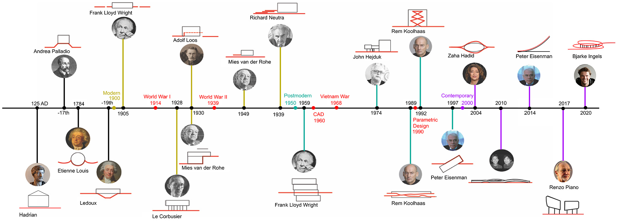
Timeline represents the development of physical building and ground designs over the last 100 years.

Figure 2.

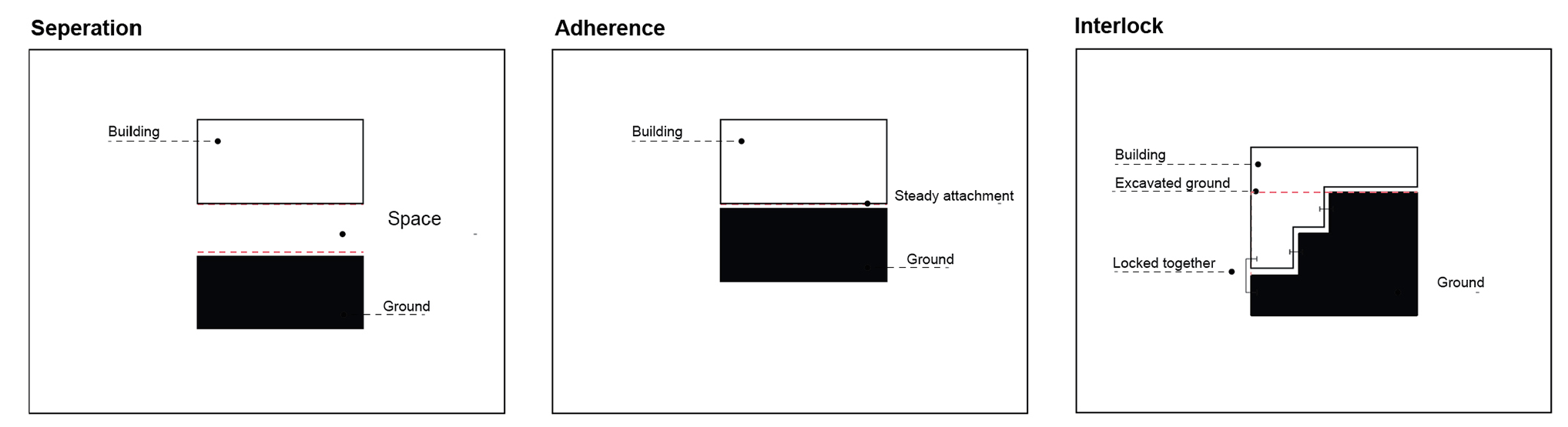
Main building and ground categories.

4. Related work

Derix and Jagannath¹⁵ developed ways to construct spatial typologies by associating spatial attributes with layouts. A building floor plan underwent analysis using isovists, centrality, and visual connectivity concepts.¹⁶ The model facilitates an experience-based approach to architectural and urban design by determining types and sequences of user experiences across buildings instead of strict typologies. To develop a reconfigurable exhibition space plan, Harding and Derix¹⁷ used a two-stage neural network and spectral graph theory as a spatial pattern recognition tool. Due to their ability to act as a spatial pattern recognition tool, a two-stage neural network and spectral graph theory were used by Harding and Derix to develop an exhibition plan. The researchers utilized spatial adjacencies to construct and classify plans and reduced the graph by finding its “graph spectrum” to facilitate its representation as a synaptic vector in feature space. The result of such an approach is that comparing graphs becomes significantly easier. A particularly noteworthy aspect of their research is that they used this approach for automatically generating spatial layouts using a repulsion algorithm combined with a diagram that distributes graphs evenly on a boundary plan. To maintain node adjacency, topological connections were simulated as springs.¹⁷

Beetz¹⁸ has researched the use of graph databases for harmonized distributed concept libraries to build information models. He aims to create “flexible, granular, and cascading concept libraries for the building industry.” The purpose of this research is to standardize the input data for graph neural networks. Tamke¹⁹ has investigated supervised and unsupervised ML approaches to deduce implicit information in (BIM). His platform can extract literal values, aggregates, and derived values from IFC SPF files. In addition, the system can perform geometrical and topological analysis that can detect anomalies and divide floor plans into two groups based upon their geometrical appearance. Ferrando et al.²⁰ aim to demonstrate how ML techniques may be used to identify typological and functional traits from building plans based on a data set of religious buildings. Their analysis of this data set, via the use of ML techniques, allows them to determine whether these buildings are mosques or monasteries and derive other such insights into the connections between typology and spatial connectivity within them. This proposed method for classifying buildings based on their spatial structures has achieved high levels of accuracy. Although this research data set focuses on religious complexes, they are confident that this approach can be applied to other buildings and help answer other architectural questions.

4.1. GCNNs

In 2014, Bruna²¹ introduced graph neural networks, demonstrating how to apply neural networks or deep learning to graphs. In 2018, Xie and Grossman²² proposed a crystal graph neural network (CGCNN) that can help ascertain crystal atom properties. During studies, CGCNN accurately predicted eight properties of crystals. A multi-GCNN was proposed in 2018 by Chai et al.²³ to predict bike flow within bike-sharing stations. By reducing the prediction error, their model has outperformed state-of-the-art prediction models. Using a diffusion recurrent neural network (DCRNN), Li et al.²⁴ proposed a deep learning framework for a traffic forecasting algorithm that incorporates both spatial and temporal dependent variables in traffic flow. Yu et al.²⁵ proposed graph convolutional networks that have consistently outperformed the state-of-the-art baseline based on real-world traffic data sets. In relation to various real-world traffic data sets, Kipf and Welling²⁶ presented a scalable approach to learning from graph-structured data in 2019. Their model scales linearly and can encode both local graph structures and features of nodes. On data sets in the domain of citation networks, they found that their approach significantly outperformed related methods. GCNN has been successfully applied in numerous different domains. However, their application in the architecture domain remains comparatively recent.

4.2. DGCNNs

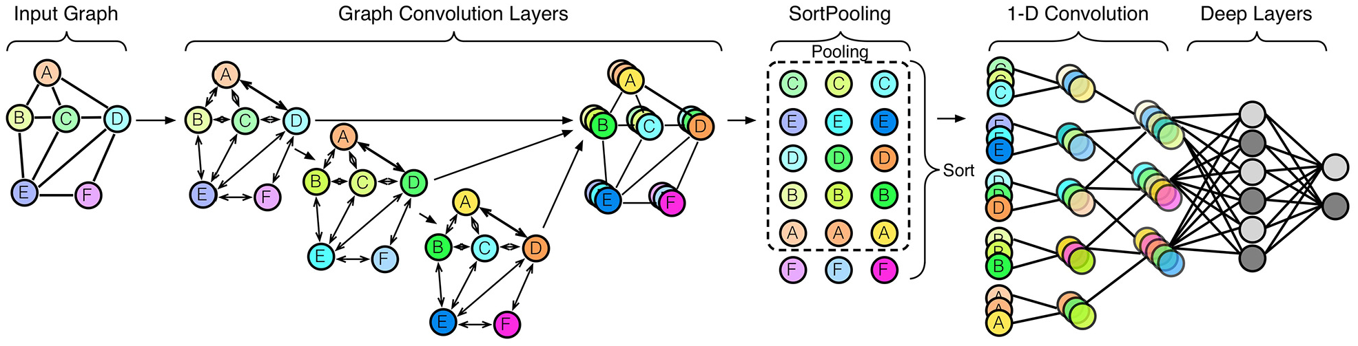
In 2018, Zhang et al. established an end-to-end DGCNN. Such a network can accept arbitrary graphs with no requirement to convert them into fixed dimension vectors utilizing feature engineering.¹⁰ DGCNN achieves this goal by sending the input graph through numerous graph convolution layers where node data propagates between neighbors. Next, an additional layer positions the graph’s vertices in a compatible sequence; the vertices then undergo input into a conventional convolutional neural network (Figure 3). By placing the vertices in order instead of summing them up, DGCNN retains more data, which, in turn, allows it to acquire information from global graph topology. In addition, Zhang et al. offer theoretical proof that in DGCNN, should a pair of graphs prove isomorphic with matching structures, their graph representation, following an assortment of the vertices, remains as it is. This situation bypasses the requirement to conduct further expensive algorithms to canonize the graph. In comparison to kernel-based methods for learning on graphs, DGCNN achieves more notably accurate results on benchmark graph classification data sets. In 2020, Jabi and Alymani used a DGCNN to classify a 3D data set of an urban block with different typological forms. Jabi and Alymani’s model reached a high prediction accuracy result (84.33%). We followed a similar approach in this paper but used a different data set and significantly different classification aim. The experiments in this paper used different labeling schemes and compare this novel workflow to other approaches.²⁷

Figure 3.

The general structure of DGCNN (re-presented after Zhang et al.¹⁰ and Jabi and Alymani²⁷).

5. Graphs

One of the best approaches to describe the connection shared by the building and the ground is to make use of graph theory. Graph theory uses mathematical structures to model relations between objects. A simple graph G comprises a set of points called vertices V(G), and lines called edges E(G) that join pairs of vertices. The degree of a vertex in a graph is the number of edges connected to it. Vertices connected by an edge are known as adjacent vertices. Similarly, the edges that share a common vertex are known as adjacent edges. Two graphs which have identical structure with respect to which vertices are connected by edges are known as isomorphic graphs.²⁸ Graphs can model numerous types of physical and biological relationships and processes.²⁹ Therefore, we used graphs in this research to model the physical building and ground relationship (for more detailed information on graph theory, please consult Voloshin³⁰).

6. Topologic

Topologic³¹ is a modeling software library created to improve space representations in 3D parametric and generative settings, as typified by Dynamo,³² Grasshopper,³³ and Sverchok.³⁴ The library follows the notion of non-manifold topology,^11,35 and its class list features Aperture, Cell, CellComplex, Cluster, Content, Context, Edge, Face, Graph, Shell, Topology, Wire and Vertex (Figure 4). A Vertex represents an area in a 3D space with X, Y, and Z values. Edges connect starting and ending Vertices, and Wires join together several Edges. Faces consist of a collection of closed Wires, while Shells gather Faces that share Edges. Cells comprise closed Shells, while a CellComplex gathers a series of Cells that share Faces. Clusters group Topologies of all dimensionalities. A Graph represents an information construction born of Topologies. Meanwhile, Apertures constitute a specific kind of Face anchored to a host Face. Topologies can often have other Topologies added to their Contents; such Content Topologies point back to their Context counterparts in a way that shows similarities with the connection between parents and their offspring. In addition, Topologies can have Dictionaries in which there exist numerous arbitrary key-attribute pairs.

Figure 4.

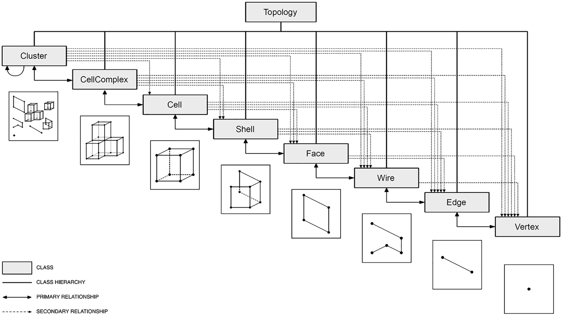
Topologic core class hierarchy.

This study will evaluate a pair of Topologic elements that have proved integral to the suggested flow of work. The first is the automated deduction of 3D topological dual graphs utilizing the Cell, CellComplex, and Graph classifications, while the second involves implanting semantic data via custom dictionaries.

Topologic can construct CellComplexes from enclosed 3D spatial units, namely, Cells that share Faces. The Cells that share Faces are otherwise known as adjacent Cells. Graph classifications and related techniques align with graph theory. Graphs comprise Vertices and Edges that join together Vertices. The Topologic library contains methods that accept Topologies as input with additional parameters and produces Graphs as output. At its most fundamental level, a dual Graph associated with a CellComplex constitutes a Graph connecting adjacent Cells’ centroids with linear Edges (Figure 5).

Figure 5.

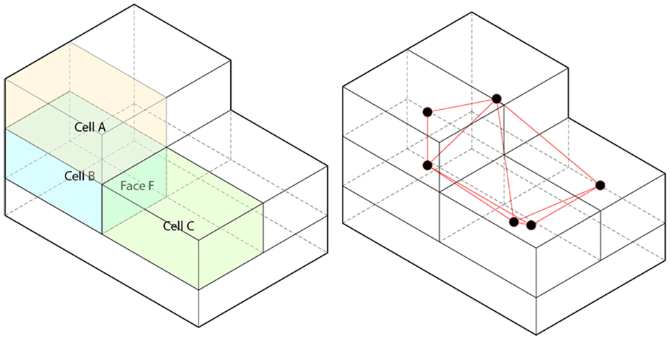
Left: an example CellComplex. Cell A and Cell B are said to be adjacent because they share Face F. Right: an example dual graph of the CellComplex. Each Cell is represented by a Vertex and the Vertices of adjacent Cells are connected by an Edge.

A dictionary is a data structure made of key/value pairs. Any identifying string (e.g., “ID,”“Type,”“Name”) acts as a key. A key’s value can be of any data type (e.g., float, an integer, a string or a list). Topologic enables the embedding of arbitrary dictionaries in any topology. When topologies undergo geometric operations (e.g., slicing a Cell into several smaller Cells, thereby creating a CellComplex), the dictionaries of operand topologies are transmitted to resulting topologies. Furthermore, creating a dual graph from a Topology sees the dictionaries of the constituent topologies transferred to their corresponding vertices. We use this capability to label the vertices in the dual graph.

7. Experimental case study

For the experimental case study, we created prototype rules around the building and ground relationship based on built architectural precedents. We then used Grasshopper and Topologic to generate various 3D parametric models and their associated topological dual graphs of the building and ground relationship (Figure 6).

Figure 6.

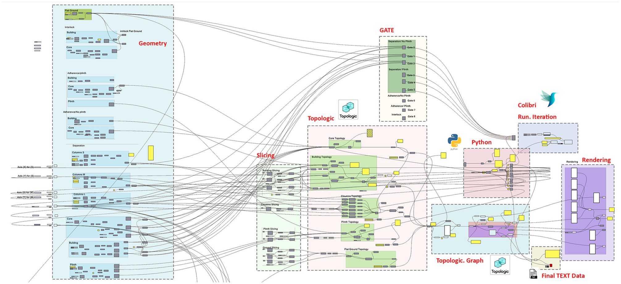
Grasshopper definition of generated 3D parametric models and their associated topological dual graph.

The ground plate was fixed in size. The plinth was then dimensioned to be a percentage of the ground plate with equal offsets on all sides. The building geometries were then placed with appropriate offsets and spacing. The height of the building was varied. Finally, the building geometries were subdivided internally into a grid of cells. It is important to note that the internal sub-division of the building was designed to aid the neural network in distinguishing structures of different heights rather than to provide room-level detail.

The rules we created were based on the main building and ground relationship, which is divided into three categories:

Separation (of ground, building, core, columns, plinth).

Adherence (of ground, building, core, plinth), and

Interlock (of ground, building, core).

Three tasks were required to create a data set. The first task was to label the overall graph. Separation is when the building is elevated from the ground on columns or on a plinth and columns. Adherence refers to the buildings that are set directly on the ground or on a plinth which in turn rests on the ground. Finally, interlock refers to buildings that overlap with the surrounding topography. The second task was to label the vertices. DGCNN required the labeling of both the overall graph and each vertex in it; for this data set, the vertices were labeled according to five categories: Ground (0), Plinth (1), Columns (2), Building (3), and Core (4) (Figure 7). The generative algorithm is aware of the category to which the generated model belongs to as well as the node types being generated within the model. Thus, it can assign the graph label as well as the node labels correctly at the point of export to DGCNN.

Figure 7.

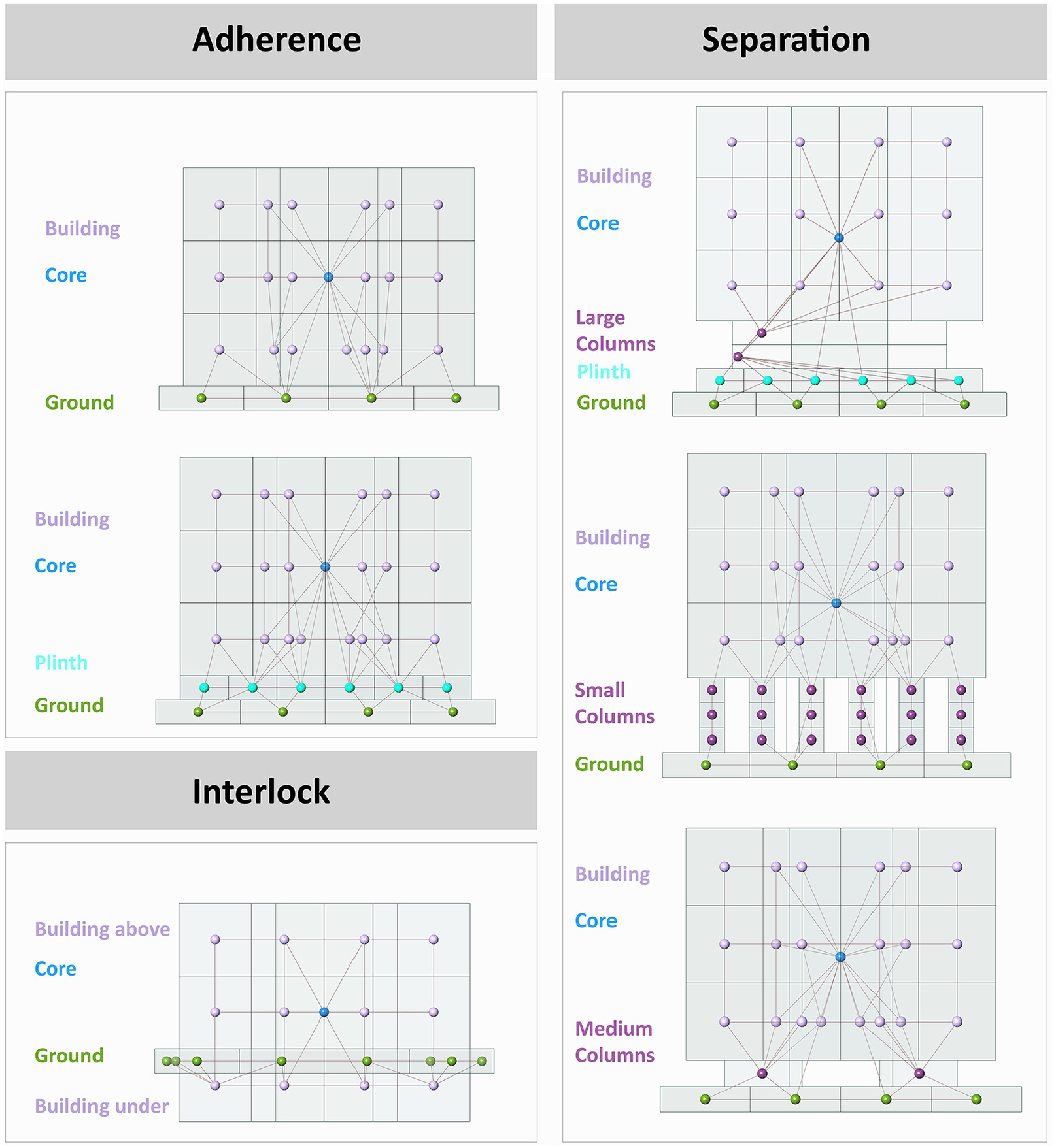
Examples of auto-generated Building/Ground configurations with associated dual graph.

The final task was to integrate the visual dataflow definition with a custom Python script to convert the 3D dual graph created by Topologic into a text file to meet the DGCNN format requirements. The first line of the text file has the total number of graphs (g). This is followed by g blocks of graphs where each block starts with a line that contains the number of vertices (n) followed by a number that indicates the classification (p) of that graph. This is then followed by a block of n vertices where each line starts with the label of the vertex (vl) followed by the indices of its adjacent vertices. The index of a vertex is implied by its line position using a zero-based numbering system (Figure 8).

Figure 8.

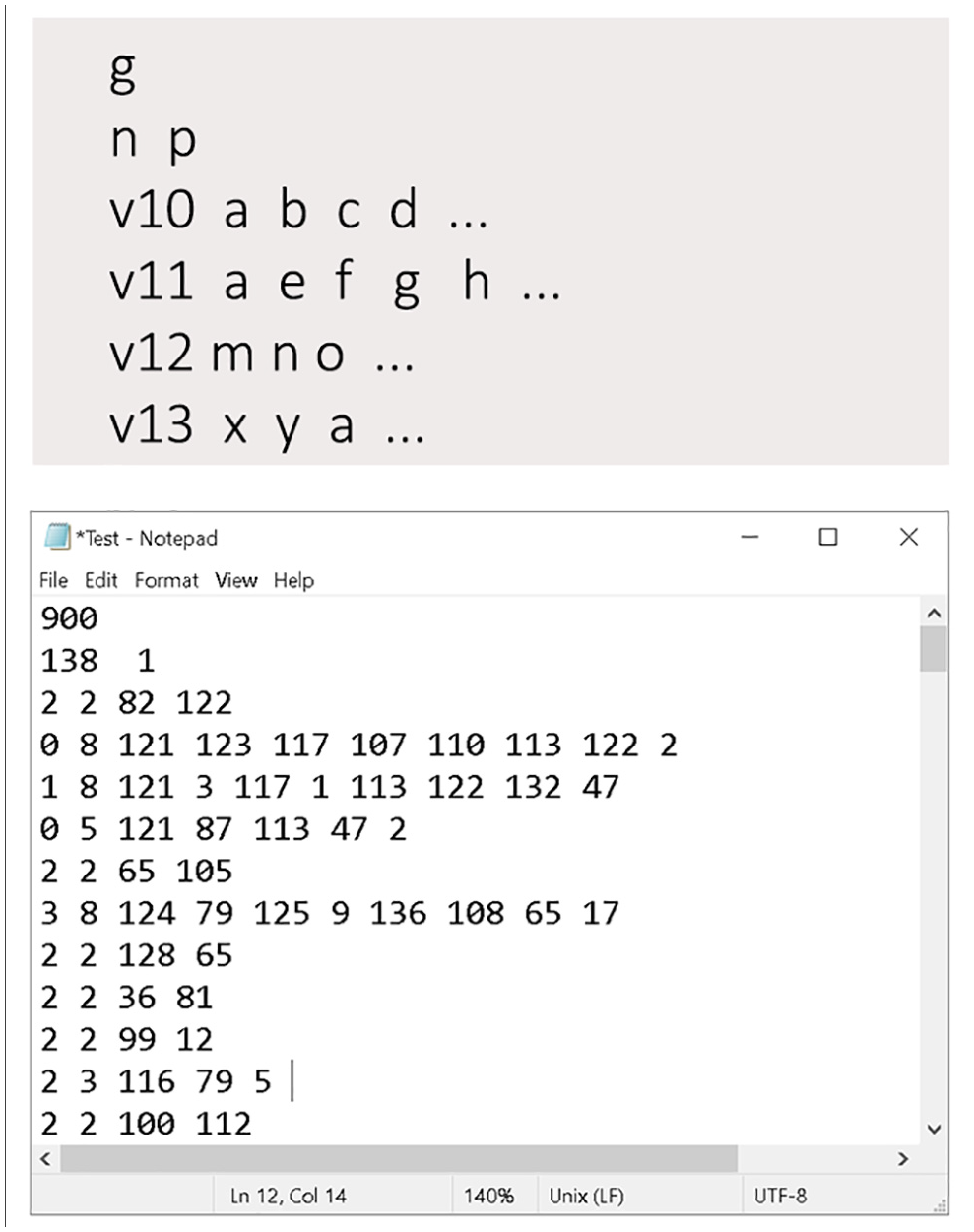
The general data set format required for DGCNN.

Since the data set in synthetically produced through iterative and nested loops, the resulting list contains sequential numeric patterns and is not random in nature (Figure 9). Thus, to avoid biased training, or the testing of only a specific level of complexity, the final list of graphs is reordered randomly.

Figure 9.

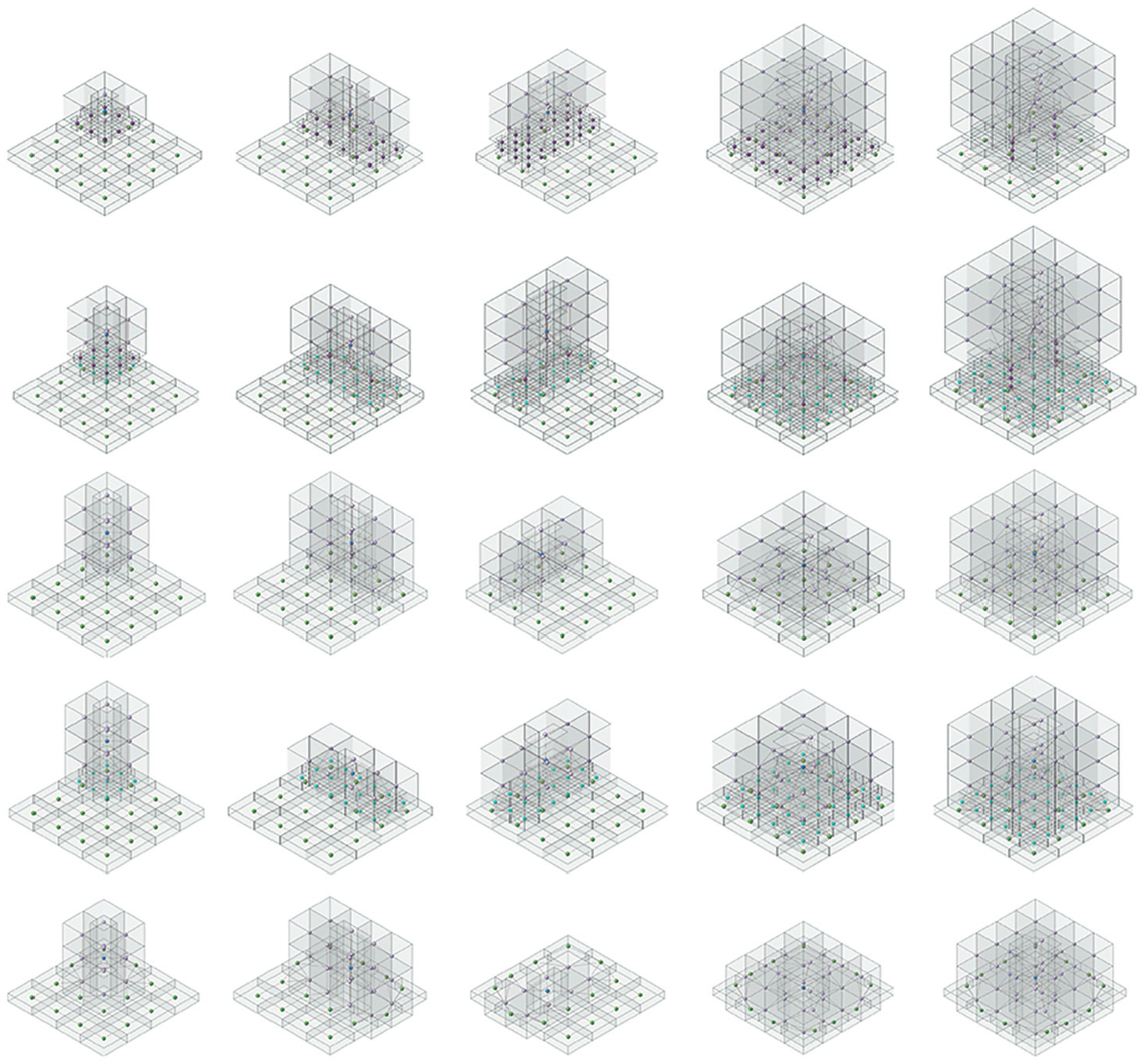
Sample of automatically generated building/ground typologies.

The produced data set totaled 900 graphs as follows:

A total of 700 Separation graphs are as follows:

Ninety building graphs separated from flat ground on small, medium, and large columns.

Ninety building graphs separated from flat ground on small, medium, and large columns, set unto a plinth.

Two hundred sixty building graphs separated from sloping ground on small, medium, and large columns.

Two hundred sixty building graphs separated from flat ground on small, medium, and large columns, set unto the plinth.

2. A total of 96 Adherence graphs as follows:

Twelve building graphs set directly on flat ground.

Twelve building graphs set on a plinth on flat ground.

Thirty-six building graphs set directly on sloping ground.

Thirty-six building graphs set on a plinth on sloping ground.

3. A total of 104 Interlock graphs:

Thirty-four building graphs interlocked with flat ground.

Seventy building graphs interlocked with sloping ground.

4. Further data set details are as follows:

The total number of vertices is 55,081.

The average number of vertices per graph is 61.

The minimum number of vertices per graph is 20.

The maximum number of vertices per graph is 197.

The total number of ground vertices is 31,772.

The total number of building vertices is 18,626.

The total number of plinth vertices is 10,689.

The total number of column vertices is 16,923.

The total number of core vertices is 900.

All experiments were run on a laptop computer running the MacOS Catalina 10.15 operating system with an Intel Core i7 Quad-Core CPU running at 2.7 GHz with 16 GB of memory. DGCNN was deployed using the PyTorch Python environment.

DGCNN has the following default parameters, most of which were maintained throughout the experiments.¹⁰ The following is a summary of these unmodified parameters:

Decay parameter: the largest power of 10 that is smaller than the reciprocal of the squared maximum node degree.

SortingPool k: set such that 60% of the graphs have more than k nodes.

Two one-dimensional (1D) convolutional layers. The first layer has 16 output channels with a filter size of 2 and a step size of 2. The second 1D convolutional layer has 32 output channels with a filter size of 5 and a step size of 1.

The dense layer has 128 hidden units followed by a softmax output layer.

A dropout layer is added at the end with a dropout rate of 0.5.

DGCNN uses a nonlinear hyperbolic function (tanh) in the graph convolution layers and a rectified linear unit (ReLU) in the other layers. DGCNN does not use validation set labels for the training.

The neural network parameters were optimized using the Adam optimizer.

DGCNN uses a Cross-Entropy to calculate the loss function.

8. Experimental results

Initially, the whole data set was split into training, validation, and testing sets. The 900 graphs were divided into 35% training, 35% validation, and 30% testing. As detailed below, the number of epochs, the learning rate, and the batch size hyperparameters were varied to improve performance. The training and validation data used for tuning the hyperparameters were 630 graphs (70%).

8.1. Number of epochs

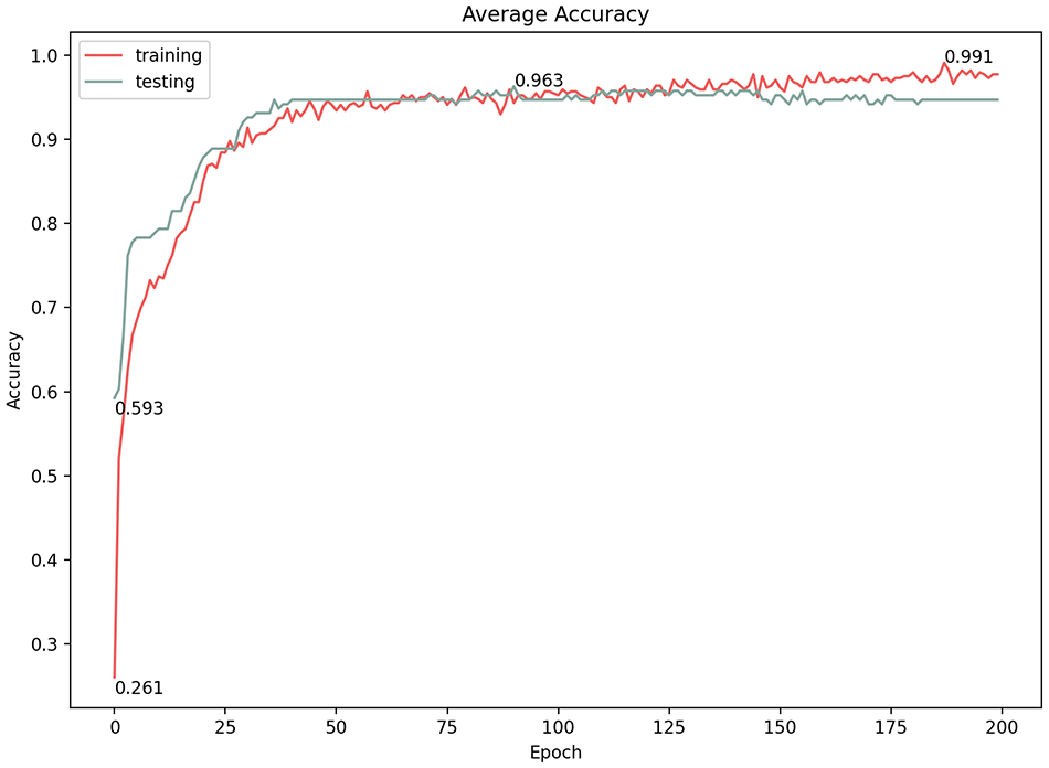
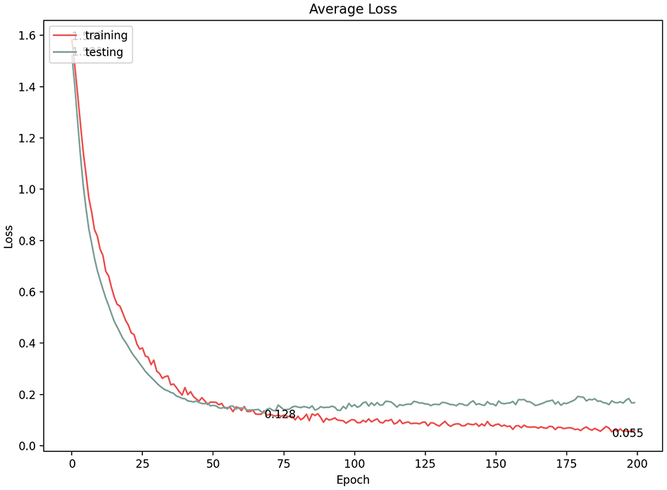
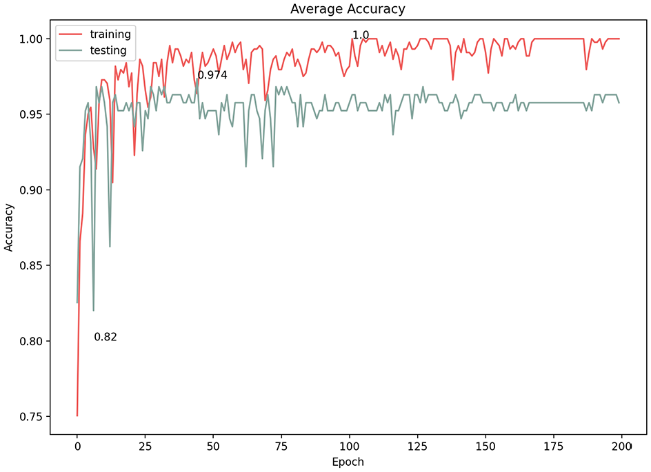
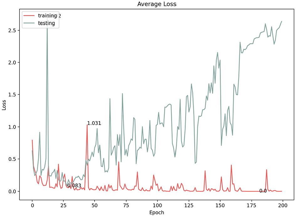
The number of epochs is the number of complete iterations through the training data set. We experimented with various numbers of epochs and found that the best classification average accuracy result was at 200 epochs (96.3%) with a 0.128 loss. Exceeding that value (i.e., 250 epochs and more) resulted in no change in the classification accuracy, although the loss gradient was significantly (Figures 10 and 11), which indicates that the model became over-fitted (Figure 10). The model started learning and improved dramatically from the first few epochs, but the accuracy level tapered after reaching approximately 200 epochs, meaning that the model stopped learning after that point.

Figure 10.

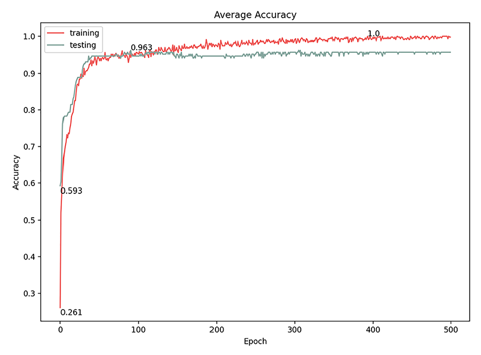
Average accuracy of 500 epochs model.

Figure 11.

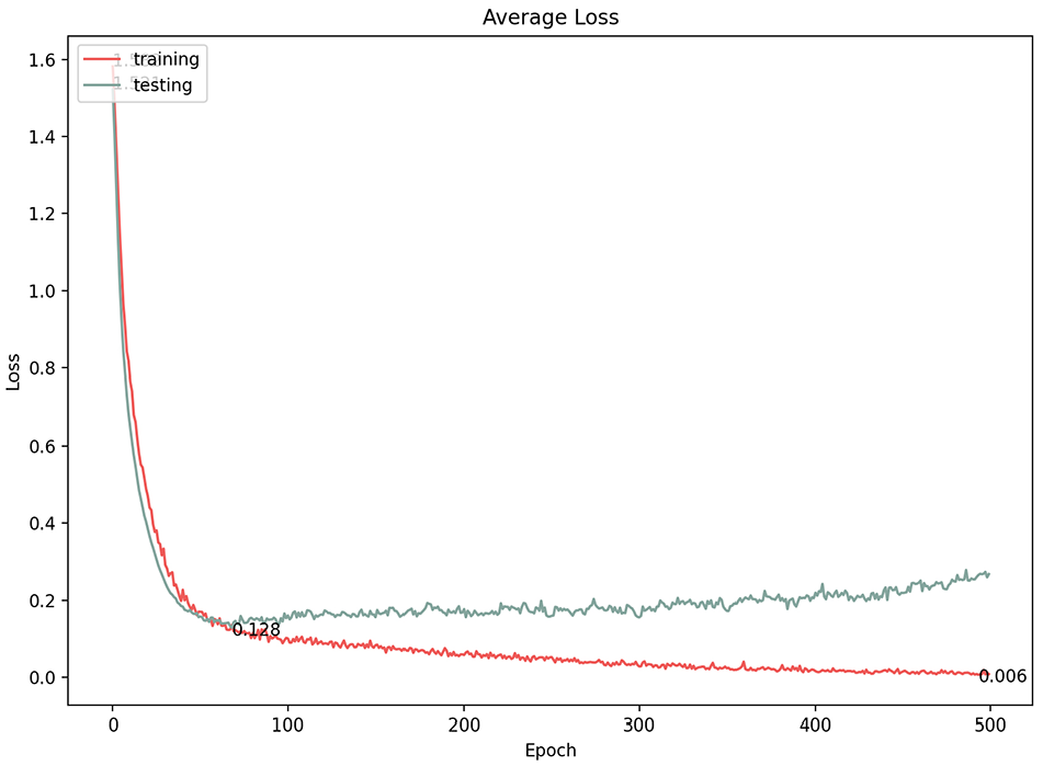
Average loss of 500 epochs model.

8.2. Learning rate

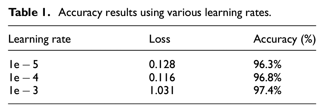
In convolutional neural networks, the learning rate is the amount by which the model parameters are updated at each optimization step. Varying the learning rate can dramatically affect the performance of the model. We experimented with three learning rates (1e−5, 1e−4, 1e−3) and documented the results (Table 1). At first glance, all three options showed high classification results; however, a more in-depth consideration of the model performance revealed a fluctuating learning performance at the 1e−4 and 1e−3 learning rates (Figures 12 –15). The highest prediction accuracy result with an acceptable model performance (96.3%) was achieved through a learning rate of 1e−5, with the lowest error loss at 0.128 (Figures 16 and 17). Therefore, in subsequent experiments, we used this learning rate to continue improving the accuracy of the results.

Table 1.

Accuracy results using various learning rates.

Learning rate	Loss	Accuracy (%)
1e−5	0.128	96.3%
1e−4	0.116	96.8%
1e−3	1.031	97.4%

Figure 12.

Average accuracy of 1e−4 learning rate.

Figure 13.

Average loss of 1e−4 learning rate.

Figure 14.

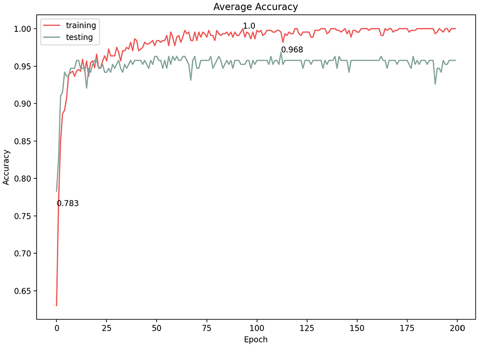
Average accuracy of 1e−3 learning rate.

Figure 15.

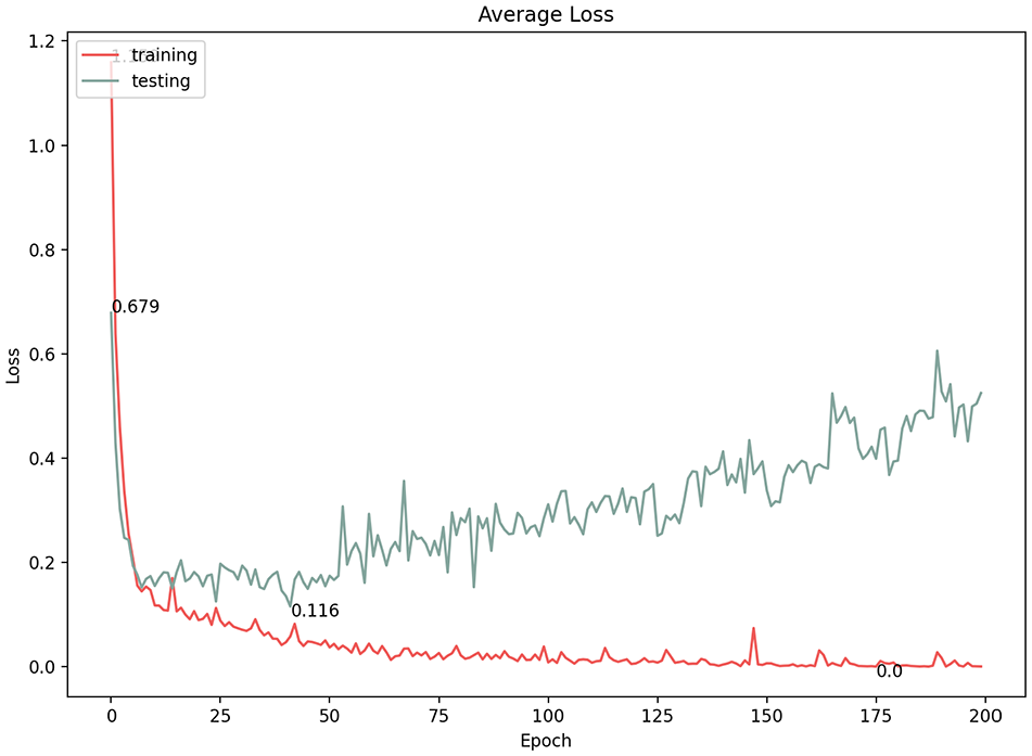
Average loss of 1e−3 learning rate.

Figure 16.

Average accuracy of 1e−5 learning rate.

Figure 17.

Average loss of 1e−5 learning rate.

8.3. Batch size

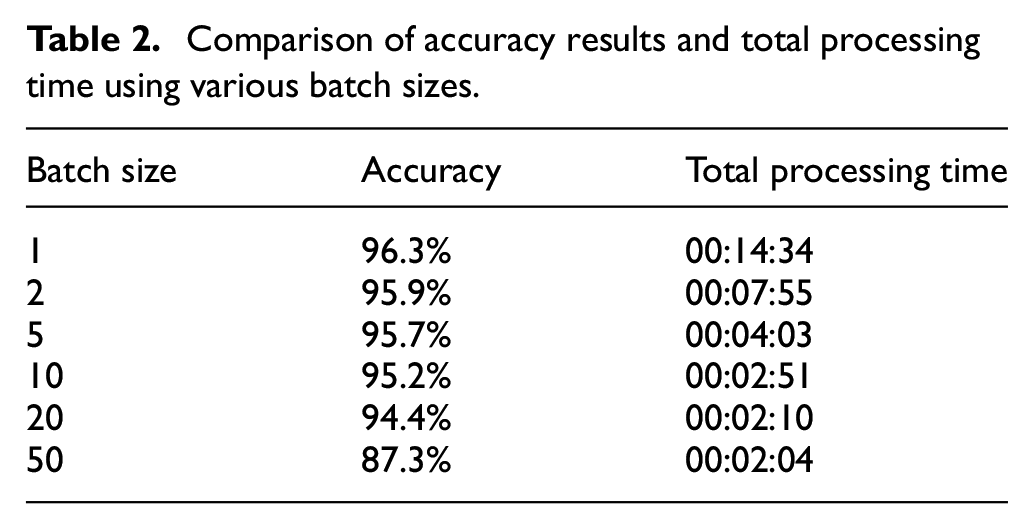
The batch size of gradient descent in convolutional neural networks controls the number of training samples to iterate through before the model’s internal parameters are updated. For this last experiment, we maintained a 1e−5 learning rate for 200 epochs while experimenting with a diverse range of batch sizes (1, 2, 5, 10, 20, and 50). The best classification accuracy was reported for a batch size of 1 (Table 2). However, a significant reduction in processing time (approximately 76%) can be achieved by increasing the batch size from 1 to 20 with a relatively modest loss in accuracy (approximately 1.9%). The associated line graph indicates the effect of the batch size on classification accuracy (Figure 18).

Table 2.

Comparison of accuracy results and total processing time using various batch sizes.

Batch size	Accuracy	Total processing time
1	96.3%	00:14:34
2	95.9%	00:07:55
5	95.7%	00:04:03
10	95.2%	00:02:51
20	94.4%	00:02:10
50	87.3%	00:02:04

Figure 18.

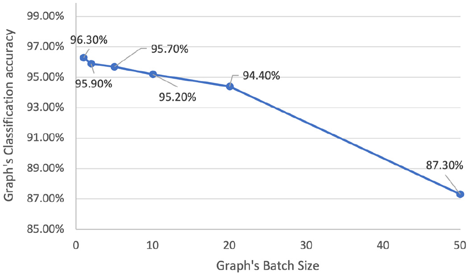
The effect of increasing the batch size on the classification accuracy.

8.4. Testing the DGCNN architecture

After tuning the hyperparameters, the best performing model was saved and tested on the test set. The parameters were as follows: epochs: 200, learning rate: 1−e5, and batch size: 1. The final test accuracy model achieved 95.6%.

Finally, the data set that we created was unbalanced, which is common for classification tasks. Moreover, our synthetic data are actually very similar/homogeneous within the same category. However, to prove the effect on the classification performance, we used an under-sampling technique to re-sample and test the final model. The new data set in this final test consisted of 253 separation, 96 adherence, and 108 interlock graphs. The final model achieved a 94.3% accuracy with 0.278 loss, which is less than the best model accuracy by only 1.4% (Figures 19 and 20).

Figure 19.

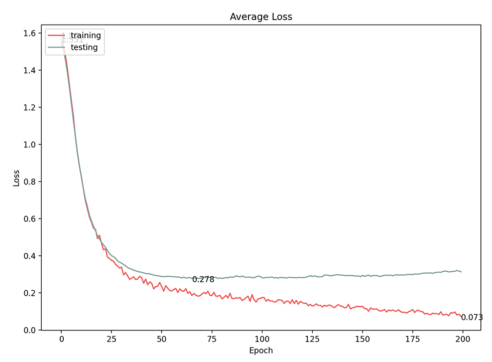
Average loss for under-sampling technique model performance.

Figure 20.

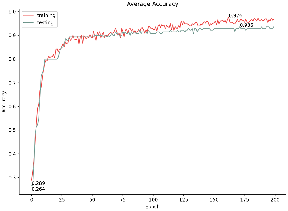
Average accuracy for under-sampling technique model performance.

9. Conclusion

This paper aimed to classify architectural topology form through a novel workflow that uses ML on 3D graphs rather than 2D images. We leveraged a sophisticated topology-based 3D modeling environment to derive dual graphs from 3D models and label them automatically. We then exported those graphs to a state-of-the-art deep learning GCNN. To discover the best accuracy rates, we experimented with different learning rates, the number of epochs, and the number of batches.

We found that the data set of 900 graphs with a testing ratio of 20%, a learning rate of 1e−5, using 200 epochs, and a batch size of 1 gave us the best prediction accuracy (95.6%). While we cannot use benchmark data sets with which we can compare our results, the results achieved in this paper are consistent with accuracy results that DGCNN achieves using benchmark data sets. This means that we have been able to leverage DGCNN’s full potential. Moreover, by improving our node labeling, these result proved superior to our last experiment on an urban block tower, which produced a prediction accuracy of 84.33%.²⁷ Our approach shows strong promise for recognizing architectural forms using more semantically relevant and structured data. Planned future work will experiment with more data sets and different building/ground topologies and compare this novel workflow to other approaches.

Due to the lack of “real” data sets, we generated synthetic data sets based on extracting building/ground relationship rules from 500 architectural precedents. We recognize that real data sets may need intervention and translation to make them amenable to dual graph extraction. Furthermore, this paper focused on the domain of an architectural object’s relation to the ground; its applicability to other typologies remains to be tested.

We have identified several new areas of research based on our findings. First, we are planning to investigate node classification rather than just overall graph classification. Second, we are planning a system that can recognize the topological relationships the designer is building in near real-time and suggest precedents from a visual database. Other future planned work includes the use of this technique as a fitness function within an evolutionary algorithm to generate and evaluate design options.

Footnotes

Appendix 1 Acknowledgements

The authors thank Architecture Andrea Mujica, Cardiff University for her help with the PyTorch programming environment.

Funding

This research received no specific grant from any funding agency in the public, commercial, or not-for-profit sectors.

ORCID iD

Abdulrahman Alymani

Author biographies

Abdulrahman Alymani is a PhD student under Dr Wassim Jabi supervision. Mr Alymani earned his MArch from Southern California Institute of Architecture (SCI-Arc). Mr Alymani is interested in wide-ranging topics in computational methods in architecture such as AI and machine learning applications in architecture, parametric design, digital design, and generative design. Alymani is interested in exploring interdisciplinary aspects of the relationship between building and ground. His work is highly interdisciplinary, and he collaborates with other academic’s areas of Computer Science, Landscape Architecture, and Urban Planning. His current research explores the relationship between building envelope and ground using machine learning (how the building meets the ground).

Wassim Jabi earned his PhD from the University of Michigan. While in the United States, he led the Association for Computer-Aided Design in Architecture (ACADIA), secured a significant National Science Foundation (NSF) grant, and taught at various universities before moving to Europe in 2008. He is currently a Reader (tenured Associate Professor) at the Welsh School of Architecture, Cardiff University where he leads the digital design area. Dr Jabi has published widely on topics ranging from parametric and generative design to the role of light in architecture and building performance simulation. He is a member of the editorial board of the International Journal of Architectural Computing (IJAC). Dr Jabi has written a book titled “Parametric Design for Architecture” (Laurence King Publishing, London). His current research is at the intersection parametric design, the representation of space, building performance simulation, and robotic fabrication in architecture. Dr Jabi has recently secured a significant grant from the Leverhulme Trust to study spatial topology in building information modeling and from the university’s internal competitive funding scheme to purchase a large six-axis high accuracy industrial robot to investigate innovative digital fabrication processes of architectural components and structures.

Padraig Corcoran is a Senior Lecturer and Academic Director of the Data Science Academy (DSA) in the School of Computer Science and Informatics (COMSC) at Cardiff University. The DSA is a recently launched collaborative project between a number of academic schools in Cardiff University which aims to ensure that Wales produces highly skilled and employable graduates in the field of data science. After completing his PhD, Dr Corcoran obtained a highly competitive Irish Research Council (IRC) 2-year post-doctoral fellowship. This in turn contributed to him subsequently obtaining a 2-year European Marie Curie International Outgoing Fellowship (IOF). Marie Curie fellowships are the flagship fellowship for leading young researchers in Europe. Dr Corcoran completed his IOF fellowship in the Computer Science and Artificial Intelligence Laboratory (CSAIL) at the Massachusetts Institute of Technology (MIT). Following completion of the above post-doctoral positions, Dr Corcoran joined Cardiff University as a lecturer in 2015. Dr Corcoran has much experience and expertise in the fields of graph theory and applied topology. He is particularly interested in applications to the domains of geographical information science and robotics.

References

Berlanda

. Architectural topographies: a graphic lexicon of how buildings touch the ground. New York: Routledge, 2014.

Porter

ZT.

Contested terrain: professional jurisdiction as a frame for analyzing the architecture/landscape divide. In: Proceedings of the 104th ACSA annual meeting conference, Seattle, WA, 17–19 March 2016.

Gröger

Plümer

. CityGML—interoperable semantic 3D city models. ISPRS J Photogramm 2012; 71: 12–33.

Kasaei

. OrthographicNet: a deep learning approach for 3D object recognition in open-ended domains, 2019, https://www.researchgate.net/publication/331008757_OrthographicNet_A_Deep_Learning_Approach_for_3D_Object_Recognition_in_Open-Ended_Domains

Sarkar

Trained 3D models for CNN based object recognition. In: Proceedings of the 12th international joint conference on computer vision, imaging and computer graphics theory and applications (VISIGRAPP’2017), Porto, SCITEPRESS - Science and Technology Publications, Lda, 27 February–1 March 2017, pp. 130–137.

Qin

Gao

, et al. A deep learning approach to the classification of 3D CAD models. J Zhejiang Univ: Sci C 2014; 15: 91–106.

Kriege

Mutzel

. Subgraph matching kernels for attributed graphs. In: Proceedings of the 29th international conference on machine learning (ICML), Edinburgh, 26 June–1 July 2012, pp. 1015–1022. New York: ACM.

Orsini

Graph invariant kernels. In: Proceedings of the IJCAI international joint conference on artificial intelligence 2015, Buenos Aires, AAAI Press, 25–31 July 2015, pp. 3756–3762.

Vishwanathan

SVN

Schraudolph

Kondor

, et al. Graph kernels. J Mach Learn Res 2010; 11: 1201–1242.

10.

Zhang

Cui

Neumann

, et al. An end-to-end deep learning architecture for graph classification. In: Proceedings of the 32nd AAAI conference on artificial intelligence, New Orleans, LA, 2–7 February 2018, pp. 4438–4445. Menlo Park, CA: AAAI Press.

11.

Jabi

Aish

Lannon

, et al. Topologic: a toolkit for spatial and topological modelling. In: Proceedings of the 36th annual education and research in computer aided architectural design in Europe (eCAADe), Lodz, 17–21 September 2018.

12.

Vitruvius. The ten books on architecture. Cambridge: Cambridge University Press, 1916.

13.

Frankl

. The secret of the mediaeval masons. Art Bull 1945; 27: 46–60.

14.

Porter

ZT.

Lecture note, Porter ZT. Theories of Ground, Lecture note, Sci-Arc, 2016.

15.

Derix

Jagannath

. Digital intuition—autonomous classifiers for spatial analysis and empirical design. J Space Syntax 2014; 5: 189–215.

16.

Hillier

Hanson

. The social logic of space. Cambridge: Cambridge University Press, 1984.

17.

Harding

Derix

. Associative spatial networks in architectural design: artificial cognition of space using neural networks with spectral graph theory. In: Gero

(ed.) Design computing and cognition. Berlin; Heidelberg: Springer, 2010, pp. 305–323.

18.

Beetz

A scalable network of concept libraries using distributed graph databases. In: Proceedings of the 2014 international conference on computing in civil and building engineering, Orlando, FL, 23–25 June 2014, pp. 955–1865. Reston, VA: ASCE.

19.

Tamke

Assessing implicit knowledge in BIM models with machine learning. In: Proceedings of the design modelling symposium: modelling behaviour, 2015, https://doi.org/10.1007/978-3-319-24208-8

20.

Ferrando

Dalmasso

Mai

, et al. Architectural distant reading using machine learning to identify typological traits across multiple buildings. In: Proceedings of the 18th international conference CAAD futures, Daejeon, South Korea, 26–28 June 2019.

21.

Bruna

Spectral networks and deep locally connected networks on graphs. In: Proceedings of the 2nd international conference on learning representations (ICLR; ed Y

Bengio

LeCun

), Banff, AB, Canada, 14–16 April 2014.

22.

Xie

Grossman

. Crystal graph convolutional neural networks for an accurate and interpretable prediction of material properties. Phys Rev Lett 2018; 120: 145301.

23.

Chai

Wang

Yang

Bike flow prediction with multi-graph convolutional networks. In: Proceedings of the 26th ACM SIGSPATIAL international conference on advances in geographic information systems, Seattle, WA, 6–9 November 2018, pp. 397–400. New York: ACM.

24.

Shahabi

, et al. Diffusion convolutional recurrent neural network: data-driven traffic forecasting. In: Proceedings of the 6th international conference on learning representations (ICLR’2018): conference track proceedings, OpenReview.net, Vancouver, BC, Canada, 30 April–3 May 2018, pp. 1–16.

25.

Yin

Zhu

. Spatio-temporal graph convolutional networks: a deep learning framework for traffic forecasting. In: Proceedings of the 27th international joint conference on artificial intelligence (IJCAI’18), Stockholm, 13–19 July 2018, pp. 3634–3640. Menlo Park, CA: AAAI Press.

26.

Kipf

Welling

Semi-supervised classification with graph convolutional networks. In: Proceedings of the 5th international conference on learning representations (ICLR’2017): conference track proceedings, OpenReview.net, Toulon, 24–26 April 2019, pp. 1–14.

27.

Jabi

Alymani

Graph machine learning using 3D topological models. In: Proceedings of the 11th annual symposium on simulation for architecture and urban design (SimAUD), Vienna, 25–27 May 2020, pp. 427–434. San Diego, CA: Society for Computer Simulation International.

28.

Wilson

RJ.

Introduction to graph theory, https://www.maths.ed.ac.uk/~v1ranick/papers/wilsongraph.pdf

29.

Mashaghi

Ramezanpour

Karimipour

. Investigation of a protein complex network. Eur Phys J B 2004; 41: 113–121.

30.

Voloshin

. Introduction to graph theory. New York: Nova Science Publishers, Inc., 2009.

31.

Topologic, 2019, https://topologic.app

32.

Dynamo, http://dynamobim.org

33.

Grasshopper Plugin, https://www.rhino3d.com/download/

34.

Sverchok, https://www.blender3darchitect.com/modeling-for-architecture/getting-started-with-sverchok-for-3d-modeling/

35.

Aish

Jabi

Lannon

, et al. Topologic: tools to explore architectural topology. In: Proceedings of the advances in architectural geometry (AAG), Chalmers University of Technology, Gothenburg, Klein Publishing GmbH, 22–25 September 2018, pp. 316–341.

Graph machine learning classification using architectural 3D topological models

Abstract

Keywords

1. Introduction

2. Motivation

3. Building and ground relationship

4. Related work

4.1. GCNNs

4.2. DGCNNs

5. Graphs

6. Topologic

7. Experimental case study

8. Experimental results

8.1. Number of epochs

8.2. Learning rate

8.3. Batch size

8.4. Testing the DGCNN architecture

9. Conclusion

Footnotes

Appendix 1

Acknowledgements

Funding

ORCID iD

Author biographies

References