
Abstract
This paper documents the workflow and supporting technologies that a large system dynamics model, the biomass scenario model, employs to streamline the data preparation, simulation, quality control, and analysis process at the National Renewable Energy Laboratory. The workflow centers on automation of routine aspects of the flow of data between data stores, simulations, and visualizations. It enforces quality checks on data, reproducibility of computations, and traceability of results, while maintaining complete archives of modeling and analysis artifacts. The resulting frictionless simulation/analysis environment supports large-scale sensitivity analysis, interactive creation of ensembles of simulations, and rapid visualization-based exploration of simulation results.
1. Introduction
The biomass scenario model (BSM) is a well-established simulation of the biomass-to-biofuel supply chain.1–5 It uses the system dynamics methology 6 to model the potential evolution of the biofuels industry, subject to physical, technological, and economic constraints, resource availability, behavior, and policy. The BSM is currently used to develop insights into the biofuels industry’s growth and market penetration, particularly with respect to policies and incentives applicable to each supply-chain element (volumetric, capital, and operating subsidies; carbon caps/taxes; R&D investment; loan guarantees; and tax credits). Because the BSM comprises hundreds of equations, incorporates dozens of input data sources as thousands of input parameters, and generates voluminous output in the form of multi-dimensional time series, data and workflow management become complex. Furthermore, its application in support of analyses for academic publications or for decision-makers and project sponsors requires high levels of quality control, reproducibility, traceability, and archivability.
This paper first discusses the BSM workflow at a high level and subsequently describes the architecture supporting that workflow, detailing the database schema, the process for editing models, the technology for executing simulations, and the process of analyzing simulation results. Through years of refining the model simulation process, it has evolved from a typical analysis workflow to a streamlined simulation-based analysis workflow. Here, the approach is explained in detail, so that this new best-practice approach could be adopted by other simulation-based and/or system dynamics models. The approach applies generally to simulations that yield multi-dimensional time series output as a function of input parameters, and the specific implementation applies to any model using the STELLA™ simulation software, though the implementation could be readily adapted to other system dynamics simulations.
2. High-level workflow
The BSM team employs an iterative process along the lines of that shown in Figure 1. The provisional requirements for a particular analysis led to preparatory phases of modifications to the BSM model, preparation of input data, and design of initial scenarios. (We define “scenario” as a set of input data designed to coherently model a state of affairs of analytic interest. The result of executing a simulation for the scenario is called a “run” here.). The team performs a rigorous set of checks on the results of the initial simulations and refines the model, input data, and scenarios accordingly. These can include checking current scenarios against a set group of historical scenarios’ key outputs (e.g. ethanol production) to see if the magnitude of difference is within the expected range. Exploratory analysis and visualization of the results may lead to further adjustments in the preparatory phases. Deeper analysis in the exploratory, visualization, and reporting phases often causes revision of the analytic requirements, particularly as they affect the design of the scenarios. The scenarios themselves may be finely crafted cases illustrating insights into the behavior of the biomass supply chain 7 or they may be statistically designed experiments involving hundreds of thousands of simulations.8,9
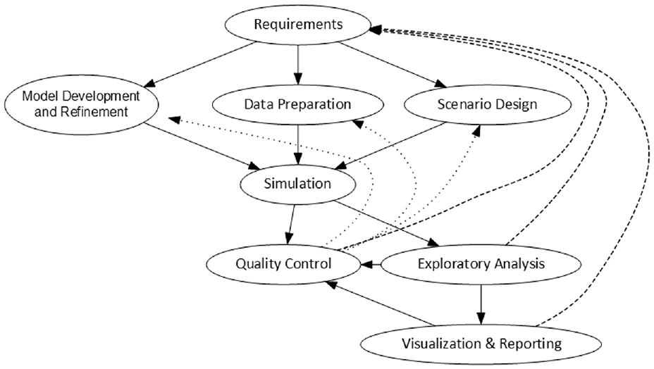
High-level workflow for analyses using the BSM: This highly iterative process begins with requirements definition and flows toward analysis products, but intermediate steps are refined to improve quality and develop insightful analyses.Source: NREL.
Throughout the process of analysis and exploration, artifacts of inputs, outputs, and visualizations are tracked and archived to ensure the traceability and reproducibility of results that are essential for analytic endeavors and for workflow and team-communication efficiencies. This not only supports the retrieval and reproduction of results long after they were first generated, but also the reproduction of the original context around the earlier analysis, so that analysts can fruitfully continue exploration, scrutinize earlier work, and elaborate upon the previous scenarios. It enhances the “team memory” of the project by concretizing the pasts’ realizations of the workflow.
3. Architecture
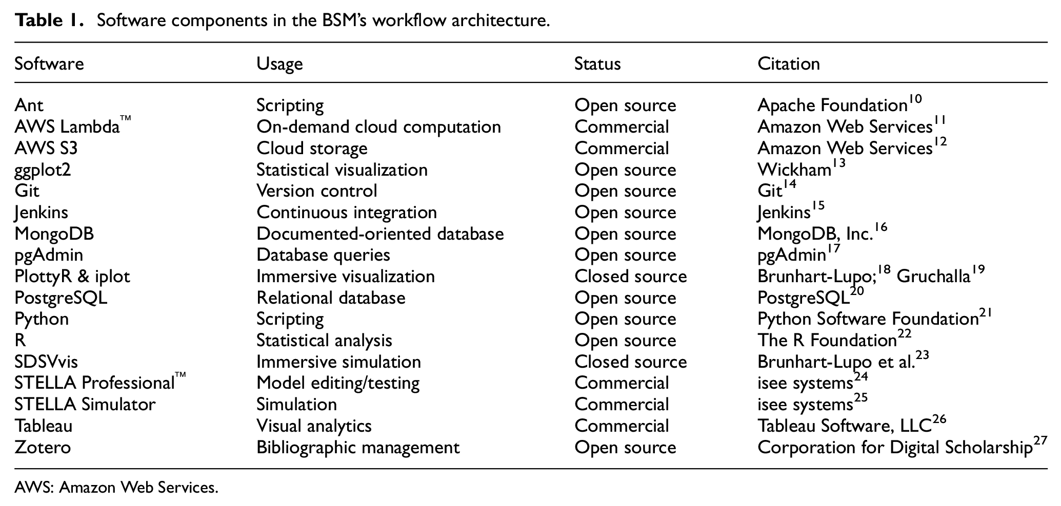
The simulation workflow relies on a suite of software tools, including databases, simulators, and visualizers (see Table 1 and Figure 2). These tools aid in moving the workflow from a historically typical one to a streamlined simulation-based workflow for performing agile analysis. For a tangible example, we point to the BSM model and corresponding infrastructure that supports model simulations. All versions of the BSM model and artifacts related to its data preparation and analysis reside in a Git repository. A PostgreSQL database holds all input data, model results, and scenario and model metadata. AWS (Amazon Web Services) S3™ (Simple Cloud Storage Service) stores backups, and Zotero stores bibliographic data. Commercial (Tableau™), open source (ggplot2), and in-house (SDSVvis, PlottyR, iplot) tools provide visualizations. Simulations use STELLA. Data analysis is done using either PostgreSQL or R. Automation and scripts (Ant, Jenkins, Python) accomplish the central portions of the dataflows in Figure 2, but data preparation and analysis use ad hoc and idiosyncratic processes.
Software components in the BSM’s workflow architecture.
AWS: Amazon Web Services.
Major components in BSM’s dataflow architecture: The dotted boxes delimit main phases of the workflow; within those, 3D boxes represent software tools, cylinders represent data stores, rectangles with turned-in corners represent data files, and arrows point along the movement of data.Source: NREL.
3.1. Database schema
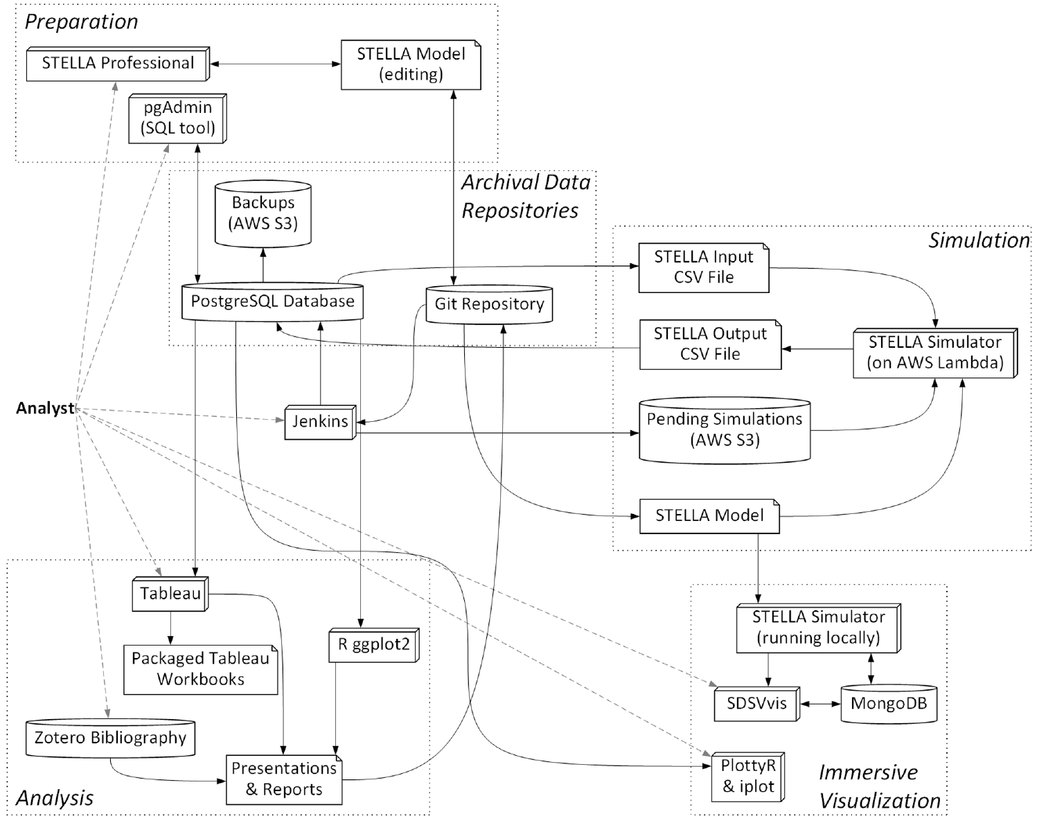
The BSM’s PostgreSQL database stores model metadata, scenario definitions, input data sets, simulations results, and other modeling artifacts. Figure 3 presents an entity–relationship diagram for the BSM schema. Jenkins’ web interface allows users to run an Ant script that transforms an XMILE format 28 STELLA model’s metadata (variables, equations, and input values—see Table 2) into SQL (structured query language) which is then inserted into the PostgreSQL database. The Revisions table associates an integer revision number and a Git hash with each version of the model. Having each model version’s metadata stored in this relational database makes it straightforward to compare model versions and perform quality assurance (QA) checks. Several standard QA checks are triggerable via the Jenkins web interface. Most of the QA checks involve verifying the correctness of input data in terms of its dimensionality (i.e. the dimensions of input arrays match the dimensions of the variable in the model), completeness (i.e. no required input values are missing), and adherence to standards (i.e. naming conventions for model variables). We have also used the model metadata to automatically generate documentation for the model.
Simplified entity–relationship diagram for the SQL schema of the BSM: each box corresponds to a table; curved blue lines correspond to relationships between tables; the boxes simply group closely related tables.Source: NREL.
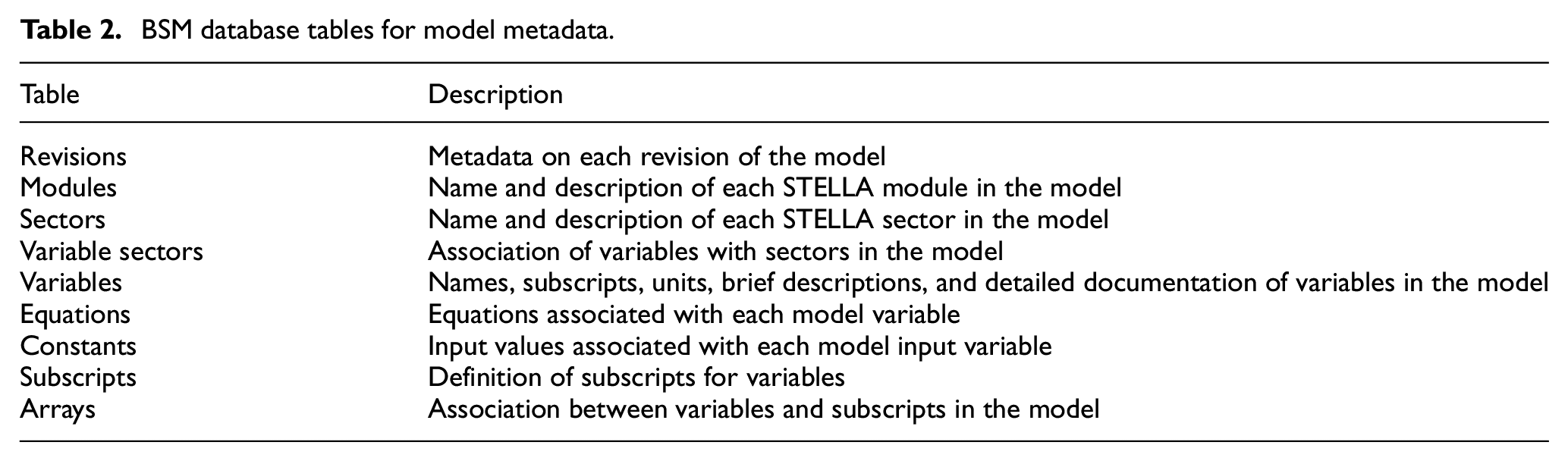
BSM database tables for model metadata.
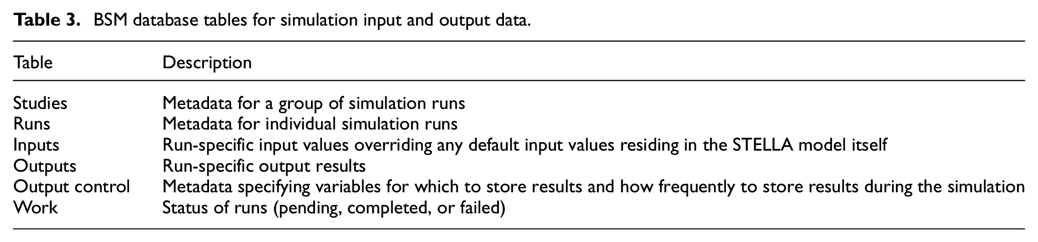
Six tables organize the input data for simulations and the output results associated with those inputs, along with metadata (Table 3). The BSM team organizes analyses into “studies,” which consist of a coherent group of simulation “runs” (results of individual simulations). Collectively, these tables and the archived version of the model itself record a precisely reproducible triad of model, inputs, and results. The BSM team’s archive of results spans over a decade and consists of hundreds of thousands of simulation results, all with provenance relating them to previous analyses and publications.
BSM database tables for simulation input and output data.
Input data sets for studies and runs may be hand crafted, generated through the statistical design of experiments, or assembled from previously prepared combinations of input parameters (called “vignettes” here). Hand-crafted inputs are developed using R, spreadsheets, or SQL, assigned a run number, and then inserted into the database. Statistically created experiments typically employ full factorial, Latin Hypercube, orthogonal array, or quasi-random designs: these are tagged with a study number and inserted from R directly into a sequence of run numbers in the PostgreSQL database. Alternatively, the input values for runs can be constructed by combining inputs, in “mix and match” style, from a selection of “variables” within vignettes (see Table 4).
BSM database tables for preparing input data sets.
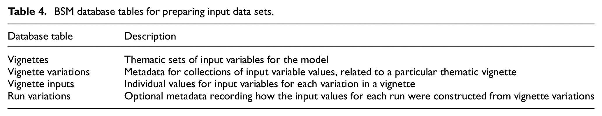
For purposes of the BSM workflow, a vignette is a thematic set of input conditions: examples of vignettes are the “Renewable Fuel Standard 2,”“Petroleum Prices,” or “Technology Cost Assumptions.” Each variation within a vignette realizes a particular state associated with the general theme of the vignette. For instance, a “Technology Cost Assumptions” vignette might have variations like “Optimistic Technology Costs,”“Standard Technology Costs,”“Pessimistic Technology Costs,”“Stagnant Technology Costs,” or “Federal Target Technology Costs.” One of the variations might be flagged as the default variation for the vignette. The vignettes and vignette variations tables encode this information, respectively. The vignette inputs table reifies each variation into the set of input values relevant for a particular version of the BSM model. A particular run can be constructed by selecting one variation from each vignette of interest; a thematic study can be constructed by collecting a group of such runs with different selections of variations for the given set of vignettes. For example, a study might consist of runs comprising all combinations of selection of either the “Optimistic Technology Costs,”“Standard Technology Costs,” or “Pessimistic Technology Costs” variation of “Technology Cost Assumptions” along with either the “Low Petroleum Prices” or “High Petroleum Prices” variation of the “Petroleum Prices” vignette, making nine runs in total. The BSM team carefully curates raw data sources into the vignettes and variations, so that meaningful new studies can be rapidly constructed from well-vetted input data.
3.2. Model editing
Analysts prepare and edit changes to the BSM using STELLA Professional™. They pull the latest master or branch version of the BSM from Git and commit changes to it there. Jenkins’ web-browser interface lets analysts perform QA functions on the model, such as finding model variables that lack documentation or pushing a new version of the model’s metadata to the PostgreSQL database. The QA process for editing the BSM varies depending on the extensiveness of the changes and whether they are made for the mainline “master” branch of the model or for a “side branch” of the model.
3.3. Simulation execution
Modelers typically make initial test runs of the BSM on laptop or desktop computers, but the automated simulation workflow described here is used for all (even early stage and internal) collaborative explorations and for all production-quality analyses. The process starts with inserting study metadata into the Studies database table, run metadata into the runs table, and input data for variables (except those having default values) into the inputs table. Jenkins can be used to insert the list of runs to be executed into the work table. Server processes monitor the work table and then create STELLA-formatted input files by querying the Inputs table using a complex SQL query, packaging those files with metadata, and then pushing them to an AWS S3 bucket that is monitored by AWS Lambda. AWS Lambda then retrieves the model to be simulated and its input data, executes the simulation, and finally stores the results in another AWS S3 bucket. Server processes next pull the results from that S3 bucket and then insert the results into the PostgreSQL database’s outputs table, also updating the status of the run in the work table. Figure 4 summarizes the interactions in this workflow.
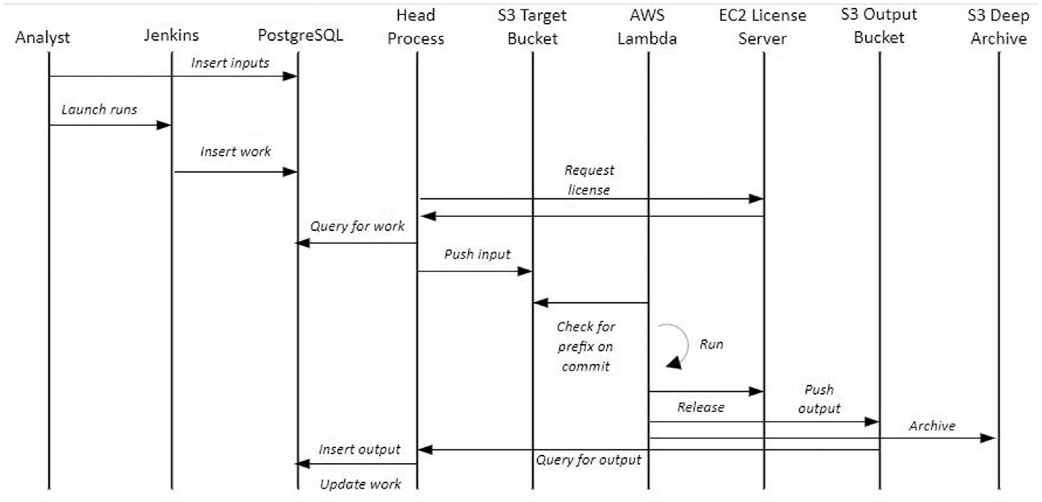
Interaction diagram for the automated execution of BSM simulations: vertical lines represent software components and horizontal arrows represent the flow of control and data.Source: NREL.
As described, the system depends on Lambda to be packaged with the most current version of the STELLA model. Creating an automated system to update the Lambda configuration automatically when a model is changed would simplify the process, but creates some extra complexity if there are potentially multiple versions of the model being used in simulation. Using Lambda to run simulations in parallel creates some complexity regardless; the system was implemented this way to work around single-system processing limitations. Having implemented a Lambda solution and having nearly unlimited compute resources at our disposal leaves us with two remaining limitations: STELLA licensing requirements and the response time of the PostgreSQL database to insert commands. Our STELLA licensing agreement limits us to a maximum of 20 concurrent processes, so that we can never exceed 20 simultaneous simulations under any circumstance. In practice, we never use more than about four processes at a time because the system becomes I/O bound performing writes to the database. Therefore, the system could be simplified considerably without sacrificing performance if all of the simulations were performed on a single host with a few processor cores available. This system could be integrated with the Git repository of model versions, making it simpler to change versions quickly or iterate on model changes. The tradeoff here is the flexibility of the system versus the overhead and expense of keeping a compute host running idle or starting it up when needed.
3.4. Analysis
The BSM analysis process varies somewhat depending on the purpose and nature of each study. The early phases of analyses invariably center on building confidence in the results, exploring provisional hypotheses, and identifying opportunities for tuning the model, input data, and scenario definition for the particular study. For this, the BSM team uses a visualization-oriented workflow relying on Tableau, a highly interactive data visualization and business intelligence tool that is well suited to the BSM’s output of multi-dimensional time series. The BSM database schema’s “long data format” normalization and table structure are nearly optimal for rapidly developing and modifying visualizations in Tableau, allowing analysts to organize variables, their subscripts, and the time dimension for single runs, groups of runs, or whole studies. Joining the vignette-definition metadata to the STELLA output allows higher-level analysis of the thematic trends in the results.
Tableau workbooks (see Figure 5) have live connections to the BSM database, so that a simple refresh of the workbook (one key press) will display the latest results when a study is being executed, enabling real-time QA activities. Because workbooks do not contain the data themselves, they can be stored and versioned efficiently in Git; however, the workbook’s data also can be incorporated into “packaged workbooks” that are self-contained archives of the data and visualizations not needing a database connection. The BSM team has evolved a semi-standard set of diagnostic workbooks that visualize key aspects of BSM output and contain QA plots that would highlight potential problems with input data, scenario design, or model structure.
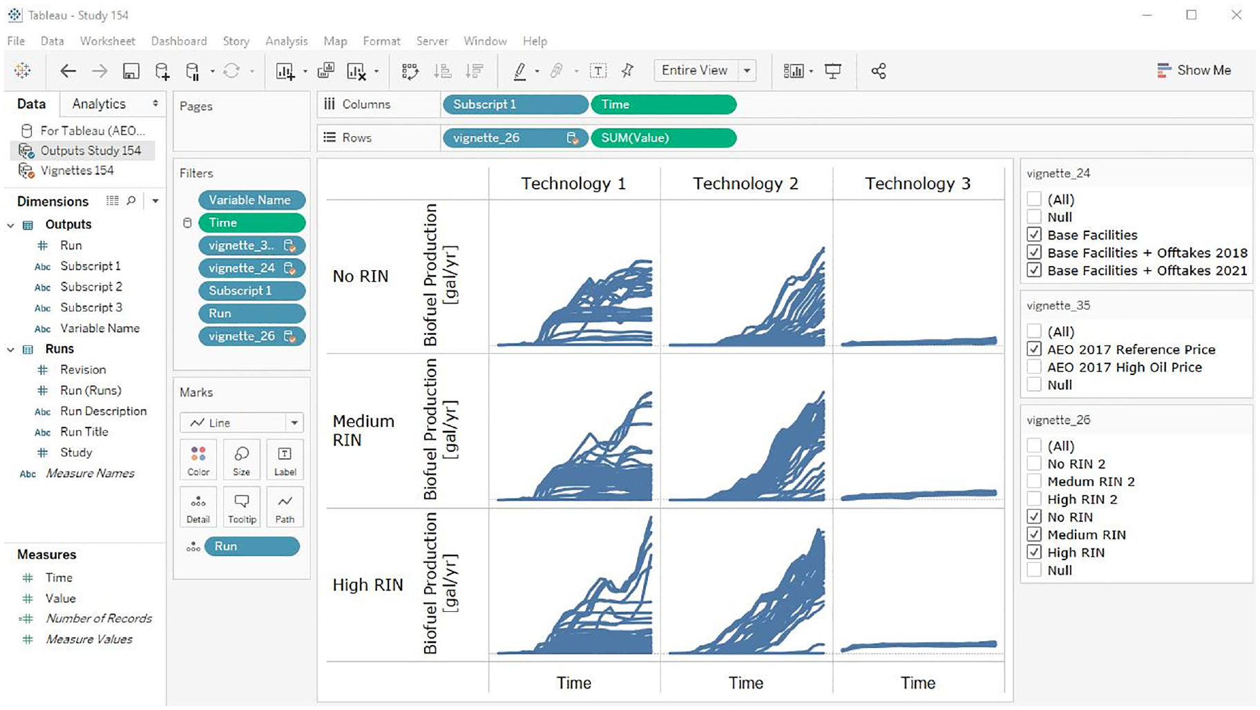
Example of interactive Tableau visualization of BSM results: the matrix of time series plots encode five dimensions of the BSM output, analysts can filter the selection of runs displayed using the checkboxes on the right, or they can interactively redesign the visualization using the controls on the left.Source: NREL.
We also use the R language and the ggplot2 graphics package for performing statistically oriented analyses and occasionally for making specialized, publication-quality graphics that would be difficult to make with Tableau. The BSM database feeds publicly available results to the publicly accessible BSM Viewer (Figure 6) when a publicly available study is selected by the BSM team to be included in the viewer through a control table in the database. 29 The BSM Viewer also has a login option, where the BSM team can share non-public results interactively with stakeholders.
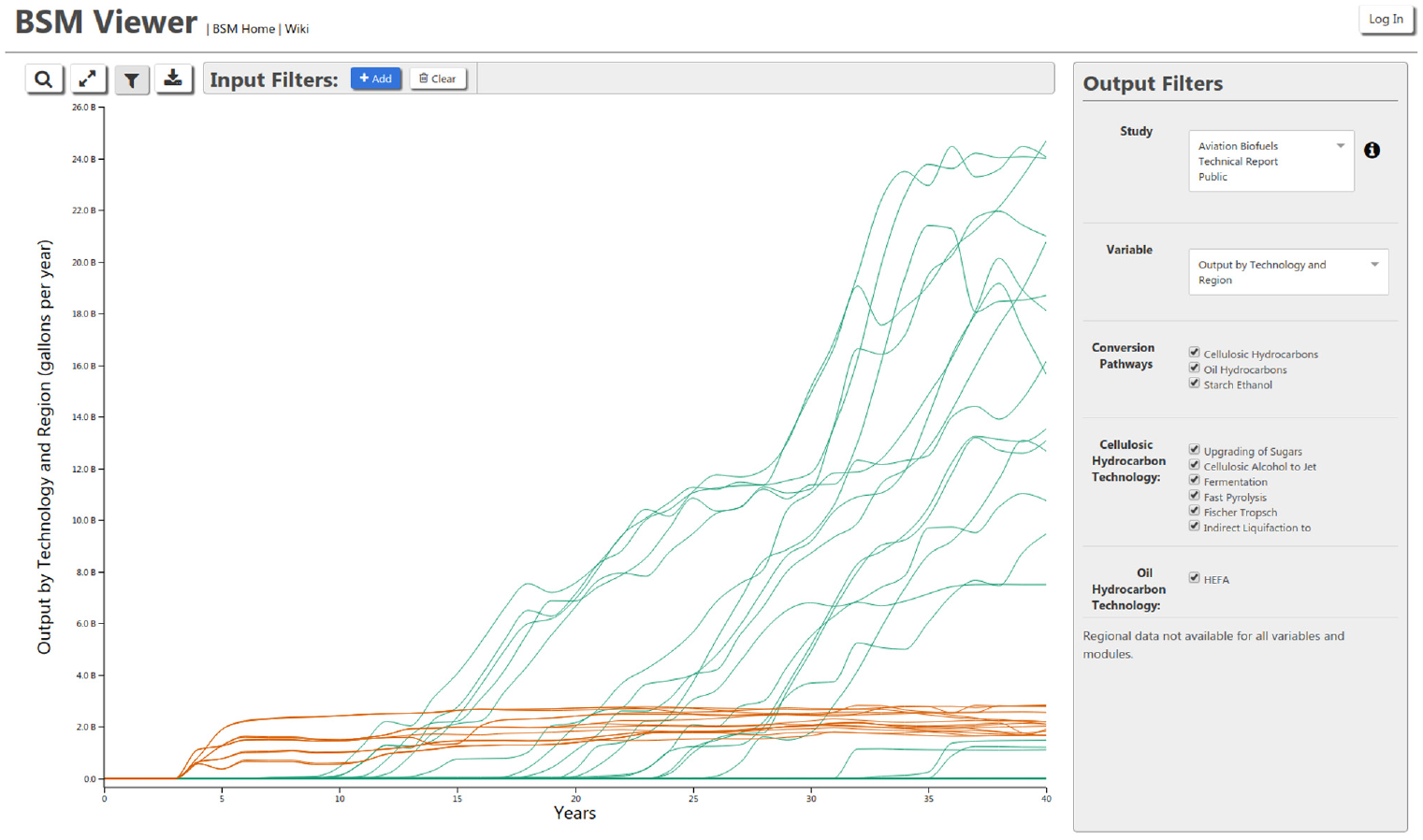
Screenshot of the BSM Viewer: visitors to <https://bsm-viewer.nrel.gov/> can interactively filter, organize, and explore the results of published BSM analyses.Source: NREL.
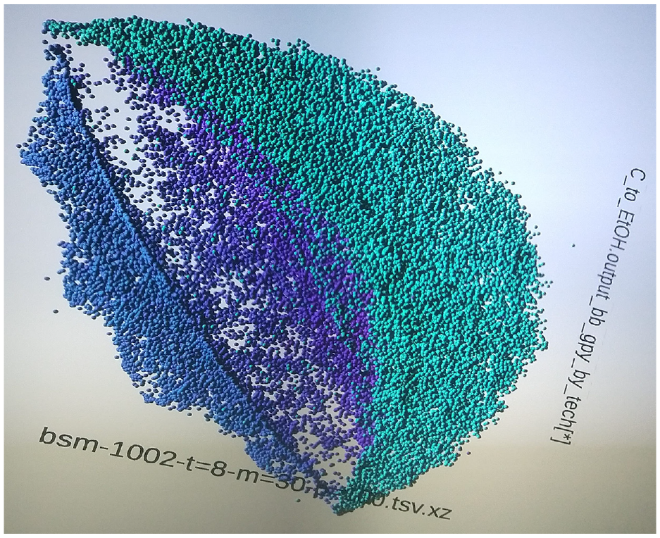
The BSM team also utilizes immersive 3D visualizations in National Renewable Energy Laboratory’s (NREL) Insight Center. 30 The SDSVvis tool 23 allows analysts to create ensembles of BSM simulations in real time and view up to 20 dimensions of correlated BSM output simultaneously for thousands of ensemble members (Figure 7). We also employ tools for web-browser-based 2D and immersive 3D exploration of the high-dimensional features of BSM output (Figures 8 and 9).31,32 The 3D tools pack more information (scenarios, data points, and dimensions) into the visualization than the 2D tools typically do, and the hands-on, immersive creation and exploration of simulation results accelerate discovery.
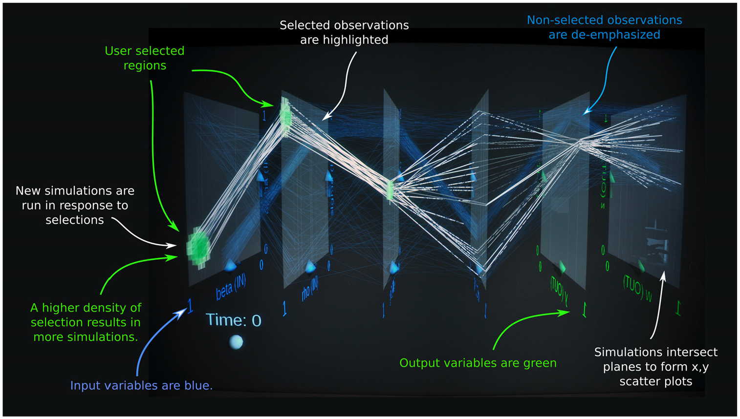
Immersive 3D “parallel planes” visual steering of BSM using SDSVvis software: 23 this visual interface to the BSM allows analysts to create ensembles of simulations by coloring input-parameter regions of interest in 3D space and then soon view the correlation between up to 20 variables of the resulting simulation output.Source: NREL.
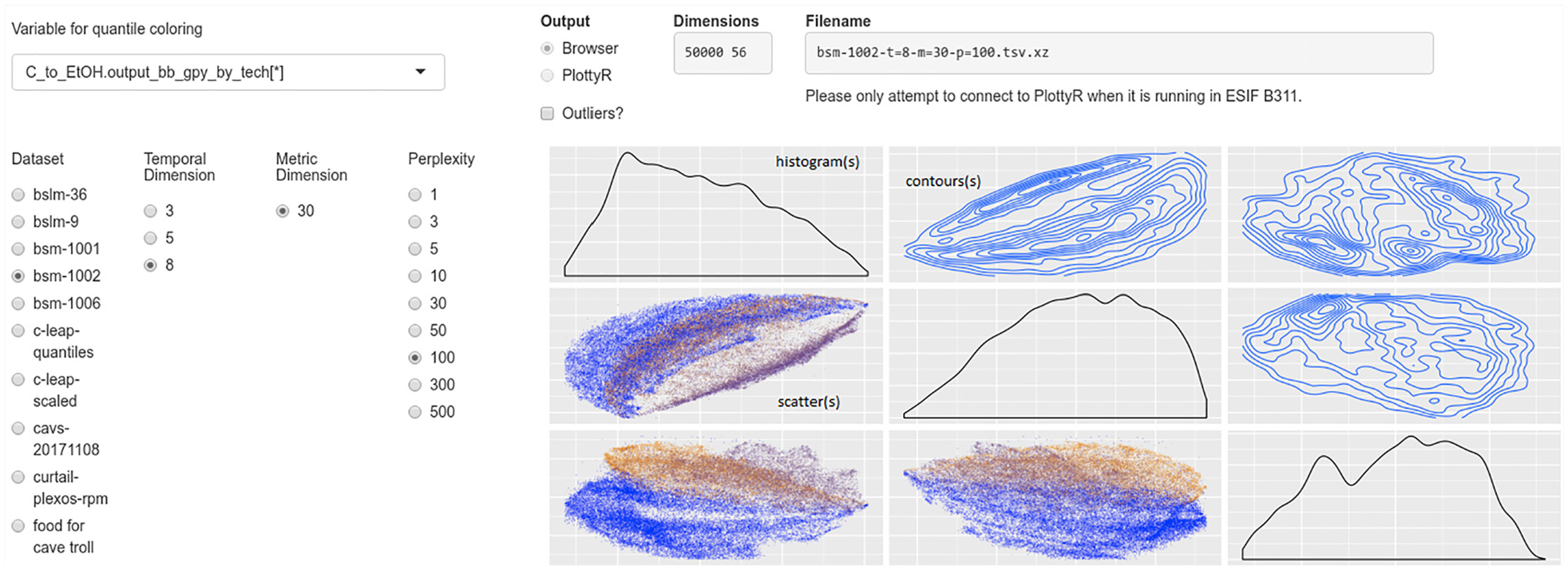
Web-browser interface to a self-organized map of BSM results: visitors to this web page can explore low-dimensional representations of the structure and features contained in the high-dimensional output of the BSM model, finding correlations between BSM variables and patterns in simulation results. The left filter panel controls the visualization which contains histograms of data (along the diagonal), contour-plots of the density of simulation results (upper right squares), and scatterplots of individual simulation runs (lower left squares).Source: NREL.
Immersive 3D visualization of a self-organized map of BSM results: this photograph shows the 3D visualization corresponding to the plots in 2D in Figure 8.Source: NREL.
These visualization-oriented analysis tools support several workflows. The most basic one emphasizes model debugging and stress testing where an analyst varies input parameters as they confirm whether the model responds with the correct qualitative or quantitative results and trends. Debugging tends to focus on input parameters close to the values of interest for a particular study, whereas, stress testing utilizes more extreme values of those same parameters. As confidence in the input data sets, scenario definitions, and model formulation/response grows, the workflow shifts toward hypotheses generation and testing, with an aim to craft and verify robust, semi-quantitative insights regarding system behavior. Exploration of the non-linear correlations between input parameters and output metrics (or just between the output metrics themselves) employs brushing techniques (visual selection of all input/output values associated with a group of runs) on ensembles of simulation runs to generate hypotheses (provisional insights) about system behavior. Analysts then visually test those hypotheses as they informally or formally execute computer experiments to verify or falsify the insights. The hypothesis generation and testing cycle iterates as insights become refined.
4. Conclusion
Over the past decade, the BSM team has evolved its simulation and analysis workflow from a traditional, iterative sequence of scenario design, input processing, execution of simulations, output processing, construction of graphics, and analysis (see top row A of Figure 10) through “visual analytics” (middle row B) toward “simulation analytics” (bottom row C).
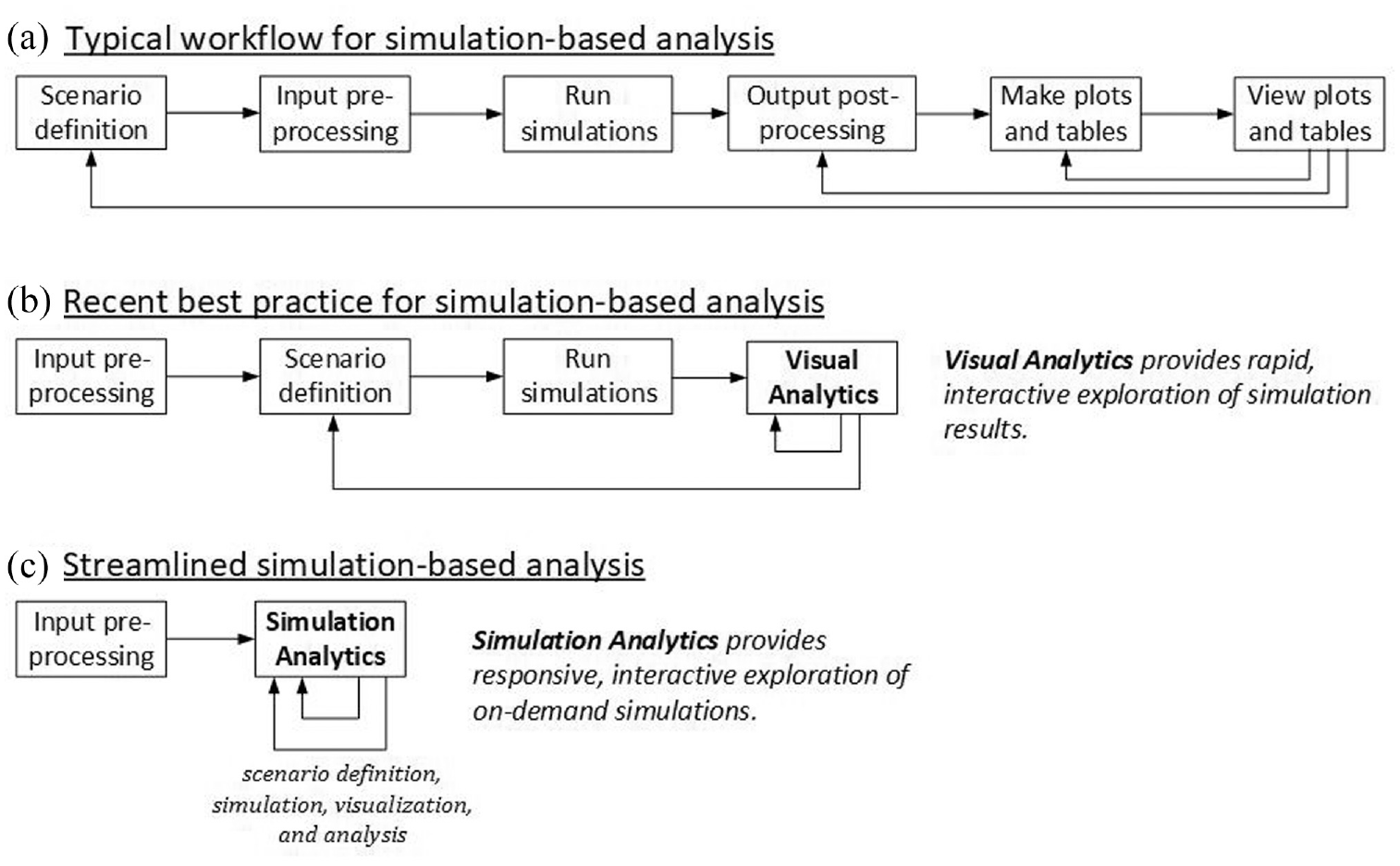
Evolution of the BSM analysis process over the past decade: (a) the workflow of a traditional analysis process, (b) a process where post-simulation phases are collapsed into interactive visual analytics, and (c) the streamlined process where scenario definition, simulation, visualization, and analysis are tightly coupled into a responsive interactive process.Source: NREL.
In conjunction with the streamlining of workflow, the BSM team has developed and implemented a dataflow that heightens quality, ensures reproducibility and traceability of results, and maintains full archives of analysis artifacts. The workflow and dataflow continue to evolve as more sophisticated and complex analyses are undertaken and as supporting technology develops.
Footnotes
Acknowledgements
The authors would like to acknowledge the review and support of this work by Alicia Lindauer and Zia Haq, US Department of Energy, Bioenergy Technologies Office. The views expressed in the article do not necessarily represent the views of the DOE or the US government. The US government retains and the publisher, by accepting the article for publication, acknowledges that the US government retains a nonexclusive, paid-up, irrevocable, worldwide license to publish, or reproduce the published form of this work, or allow others to do so, for US government purposes.
Funding
This work was authored by the National Renewable Energy Laboratory, operated by Alliance for Sustainable Energy, LLC, for the US Department of Energy (DOE) under Contract No. DE-AC36-08GO28308. Funding provided by the US Department of Energy Office of Energy Efficiency and Renewable Energy’s Bioenergy Technologies Office.