
Abstract
Regardless of its origin, in the near future the challenge will not be how to generate data, but rather how to manage big and highly distributed data to make it more easily handled and more accessible by users on their personal devices. VELaSSCo (
Keywords
1. Introduction
The Discrete Element Method (DEM) is a simulation tool used in engineering to model complex systems of particulates at the particle scale by specifying a relatively small number of microstructural parameters. DEM is very closely related to molecular dynamics (MD), an analysis tool used in chemistry, biochemistry, and materials science. 1 The largest difference between DEM and MD is the scale of interest: MD simulates the interactions between individual atoms or molecules, whereas DEM is used to simulate soils, powders, and grains at much larger scales. The fundamental algorithm for MD was proposed in the 1950s,2,3 with the related DEM methodology developed later in the 1970s. 4 Since then, DEM has become increasingly popular for analyzing the particle-scale mechanisms that underlie the complexity of the overall material response. In the most common implementation of DEM, particles are modeled as rigid bodies with finite size, inertia, and stiffness. Deformations of particles at the contact points are captured by permitting overlaps between the interacting bodies. The particle sizes usually range from microns to tens of millimeters. A timestepping algorithm is implemented and, at each successive timestep, interparticle forces are evaluated at the contact points using suitable force–displacement relations. The resultant force on each particle is calculated by summation. Newton’s Second Law is applied to determine particle accelerations based on the resultant forces, 5 which are integrated numerically to find particle velocities and displacements; hence, positions may be updated during each timestep.
DEM is capable of providing extremely detailed information about the microstructure of a simulated material and its temporal evolution. Such information is of interest to researchers working with a broad range of granular materials from minerals to pharmaceuticals. Although some barriers remain to the adoption of DEM for industrial applications, 6 its popularity continues to grow.1,7 There has been an approximately linear rate of increase in the number of DEM-related papers published since 1996. 5 The growing interest in DEM among the scientific community is further emphasized by the publication of a number of special issues of journals devoted to DEM within the past decade—for example, Engineering Computations 26(6); Granular Matter 11(5); Powder Technology 193(3); Powder Technology 248.
This interest in DEM has been driven by the increasing availability of substantial amounts of computational power, enabling fully three-dimensional simulations to be run that are of practical use. MPI-parallelized solvers such as LAMMPS 8 and LIGGGHTS 9 scale to hundreds of nodes and beyond on clusters. The popular commercial codes PFC 10 and EDEM 11 use parallel processing to exploit modern multicore architectures. Inevitably, increases in computational power and the exploitation of parallelism lead to commensurate increases in the amount of data generated by particle simulations. Although predictions that a 10 million particle problem would be considered “easy” by 2011 were optimistic, 12 the predicted continual growth of simulation size has been proved correct. The accessible timescales and number of atoms in MD simulations have closely tracked Moore’s Law. 13 A large DEM simulation now generates >1 TB of data (information about each particle and each contact in the system) with hundreds of megabytes of data per timestep. For large-scale N-body simulations, the current limitation is data post-processing, which is often done on a single workstation. This is unsustainable as the data storage requirements and CPU effort required for analyses become ever-larger.
Post-processing of particle simulations is often essential for correct and/or meaningful interpretation of the data. In particular, consider the discrete-to-continuum (or Discrete2Continuum/D2C) transformation. This applies temporal and spatial coarse graining methods14,15 to DEM simulation data in order to compute bulk quantities such as solid fraction or stress tensors that are projected onto a continuum field. A snapshot of the data at one instant appears chaotic and does not show the concealed, underlying trends that emerge over longer timescales. This computationally expensive post-processing allows the long-term behavior of scientific interest to be distinguished from short-term random and transient fluctuations. The current limitations on processing of large-scale simulations mean that often analyses are conducted with small subsets of the available data. This leads to two related problems: first, restricting the analyses to a small fraction of the data could yield misleading results; and second, some of these data that are discarded without analysis could contain results of scientific interest.
There are several papers in the literature showing the usefulness of the D2C transformation. Weinhart et al. 16 recently simulated silo discharge using DEM and applied spatiotemporal coarse graining to the data. They quantified stresses from interparticle contact forces and demarcated three distinct flow regions by comparing macroscopic fields obtained from spatial averaging. This analysis identified stagnant, highly stressed regions adjacent to the silo outlet. This indicates that, in order to achieve mass flow where the stored solids are all flowing concurrently, the silo would need to be redesigned – for example, by changing the hopper angle. Clark et al. 17 applied coarse graining to an impeller-driven mixer system to evaluate local densities, averaged velocities, and granular temperatures. The quality of mixing may be evaluated using this information; the extent to which materials are mixed can significantly affect product quality 18 and sometimes safety—for example, excipients and active pharmaceutical ingredients (APIs) must be blended thoroughly before tableting to ensure that no tablet contains a potentially dangerous surfeit of API.
Such analyses are very computationally expensive and were formerly limited to small datasets with few particles and/or timesteps. This was due to the lack of a suitable parallelized tool for distributed analysis of scientific Big Data. In this paper, we discuss the VELaSSCo software platform, aiming to address this problem. 19 This platform is developed within an EC FP7-funded project, VELaSSCo: “Visualisation for Extremely Large-Scale Scientific Computing.” VELaSSCo is a three-year project that ran from January 2014 to December 2016. The goal of VELaSSCo was to create the VELaSSCo platform for distributed post-processing and visualization of very large engineering datasets. 20 These datasets include DEM, the finite element method (FEM),21–23 and computational fluid dynamics (CFD).24–26 VELaSSCo is a consortium of seven European partners: the University of Edinburgh (UK), CIMNE, Atos Research & Innovation (both Spain), INRIA (France), Fraunhofer IGD (Germany), SINTEF, and Jotne EPM (both Norway).
The development of the VELaSSCo platform has been guided by a user panel. The panel was consulted at the start of the project to learn of their requirements for the platform, they were kept apprised of developments, and they evaluated both an early prototype of the platform and the final platform. User feedback on the prototype has been invaluable to inform its subsequent development. The user panel had around 60 members, with approximately a 70:30 balance between academia and industry. Usability testing in VELaSSCo followed a “goal, question, metric,” or GQM, approach to software metrics. 27 Two variants of the VELaSSCo platform have been created: a fully open-source version and a proprietary version which use Apache HBase and EXPRESS Data ManagerTM (EDM) as database systems, respectively. Only the open-source version is described in this paper.
The aim of this paper is to show, by means of selected use cases, how the VELaSSCo platform facilitates distributed post-processing and visualization of large engineering datasets. A comprehensive overview of the platform is provided along with a description of the D2C transformation for DEM data. Some practical guidance is provided for using the platform, while two DEM use cases demonstrate the capabilities of the VELaSSCo platform.
2. Overview of the VELaSSCo platform
The VELaSSCo platform was developed to work both with open-source and closed-source software. The open-source version is built on top of the open-source Hadoop software stack—a Java-based framework for distributed storage and processing of Big Data. The software components within the Hadoop framework include the Hadoop Distributed File System (HDFS), which stores files in a distributed, split, and redundant way for parallel access; HBase, a distributed database built on top of HDFS providing a transparent means for storing and accessing data on the cluster; YARN, which manages the computing resources and schedules jobs across the cluster; and MapReduce, which refers to the programming model for large-scale data processing. Figure 1 shows the three main layers in the architecture: the visualization clients, the Core Analytics Module, and the Data Layer.
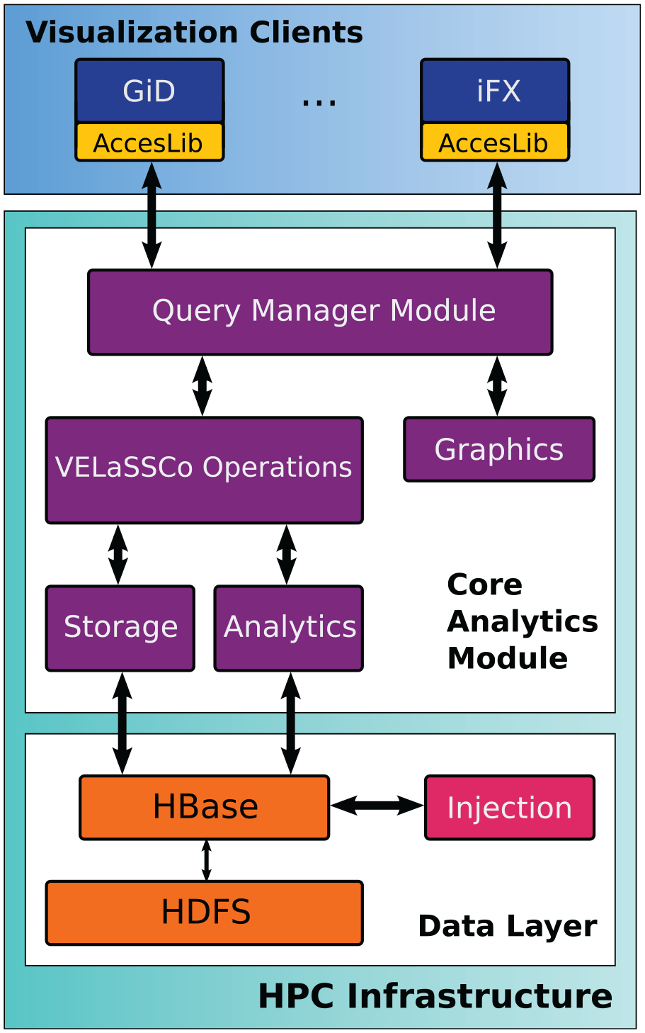
VELaSSCo open-source architecture.
2.1. Visualization clients
The visualization client triggers queries through the access library, which is the interface between the client and the platform. The complex D2C query is explained in a later section. The visualization clients (currently two: GiD 28 and iFX 29 ) implement a plugin to access the platform. Integration between components is done through a Thrift API, so the plugin implements a public API provided by the platform. The results output by the queries are returned to the clients through an internal VELaSSCo format which is designed to minimize latencies through high-speed transfer. The following requirements were considered when designing the format:
In this format, a batch of data is represented as a file. A file is a self-contained binary “blob” of data that includes all the information to display a scene. Such a file consists of two sections, a header section and a data section. The header contains a description of how the payload is handled. The data section is simply a collection of buffers. Within a C/C++ program a file could be accessed as the struct shown in Listing 1.
The internal VELaSSCo platform file format. It is used to transfer DEM/FEM meshes from the HPC infrastructure to visualization clients.
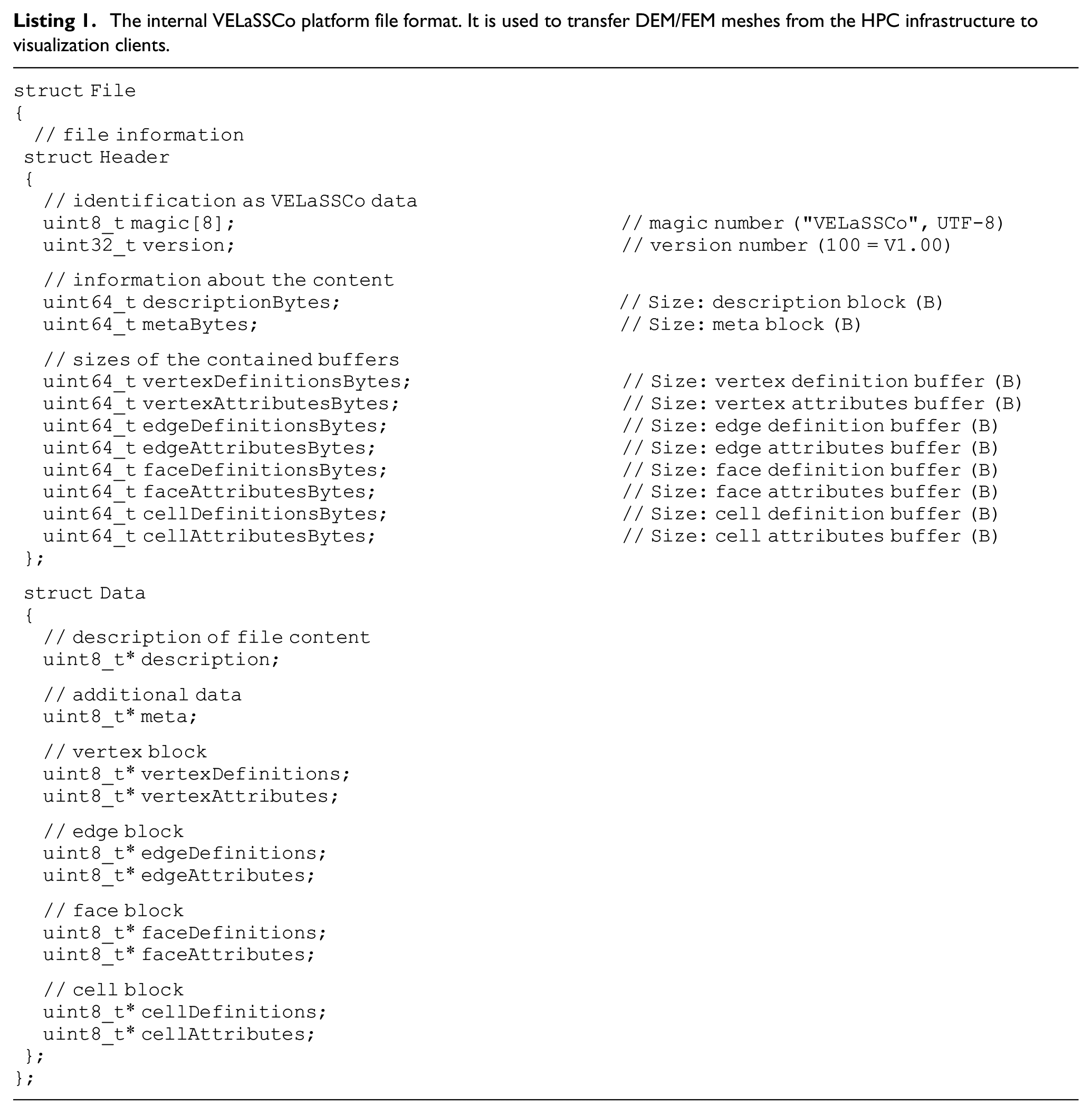
For example, transferring particles with information requires the use of vertex definitions and vertex attributes. The vertex definitions buffer keeps particle centers along with vertex attributes which store their attributes (e.g., radius). In addition, pressure, velocity, etc. can be packed into the file format sent to the client. The description buffer is responsible for implicitly informing the visualization clients about incoming file contents and how they should be interpreted.
In the case of progressive visualization (e.g., visualizing particles across different timesteps as an animation), this format does not explicitly support streaming or level-of-detail display. The intention is that in such cases data are not sent as a single file, but rather as a stream of files (which are transferred one after another). Later, files could either contain new data that replace old data (e.g., a new set of triangle strips), but they could also provide incremental data. For example, in the case of progressive meshes, new files could add new vertices and edges that are used to expand available geometries to a new detail level. How new data are to be interpreted could be defined in the description buffer.
The rendering algorithms are optimized to provide highest efficiency during rendering of the received data. In DEM cases in which the particles need to be drawn, they are received in a compact format. As mentioned before, the client can redirect it to the rendering module without any conversion. The iFX visualization client supports two rendering modes: rasterization-based and ray tracing-based. In both cases, particle data are sent to the rendering device without any conversion. Furthermore, the deferred approach 30 is utilized to improve massive mesh (e.g., very high number of particles) rendering efficiency. In addition to position, material, etc. buffers stored as G-Buffer, for each attribute, a buffer is filled during the first stage. Although rendering simulation meshes consisting of cells is done via triangulation, a more efficient approach is utilized for particle rendering. In the first approach, the GPU’s pipeline is programmed so it produces a sprite in the geometry shader for each particle. Spheres inside every sprite are ray casted in the fragment shader. 31 To improve the final result, screen space techniques such as depth darkening 32 and ambient occlusion 30 can be applied to the shaded image to improve the final image’s visual perception quality. In the ray tracing-based approach, the received data are used to produce a bounding box for each particle; then a bounding volume hierarchy 33 acceleration structure is created and used to speed up ray tracing. To get pixel-accurate results, instead of triangulating the spheres, ray–sphere intersection is done analytically. In addition, path tracing- 34 and ray tracing-based ambient occlusion can be utilized to give better perceptual clues about depth, curvature, and proximity. In the second stage of deferred shading, attribute values are mapped to a color ramp and used during lighting calculation as the geometry colors to make the final images easier to analyze.
In addition, the mesh data transferred to the client can be post-processed by existing tools in visualization clients. For example, D2C result meshes can be cut through, or streamlines can be computed on the client side to help the user get a better understanding of attribute-changing behaviors inside the mesh.
2.2. Core analytics module
The queries triggered by the visualization clients are processed by the Core Analytics Module, which retrieves and analyzes the data. This module runs on the HPC infrastructure and delivers the query results to the visualization clients. The data are compressed to avoid overloading the network. Different internal modules are in charge of the different functions:
2.3. Data Layer
The Data Layer is the deepest layer and stores and manages the data. The core of this layer is HDFS, which is responsible for data storage and distribution across regions. It guarantees data replication across the Hadoop cluster and fault tolerance. HBase is a non-relational database that works on top of HDFS and provides real-time access to the data. As it stores information with a key–value structure, all data can be easily accessed.
The simulation data can be received by the system in real time or via files, with the final data stored on disk. The injection module manages both data sources. Apache Flume is used to ingest simulation data into HBase. Once the data are stored in HBase, the injection module is able to perform some post-injection actions, such as execute a set of frequently called queries and store the results data to provide faster results to users in future queries.
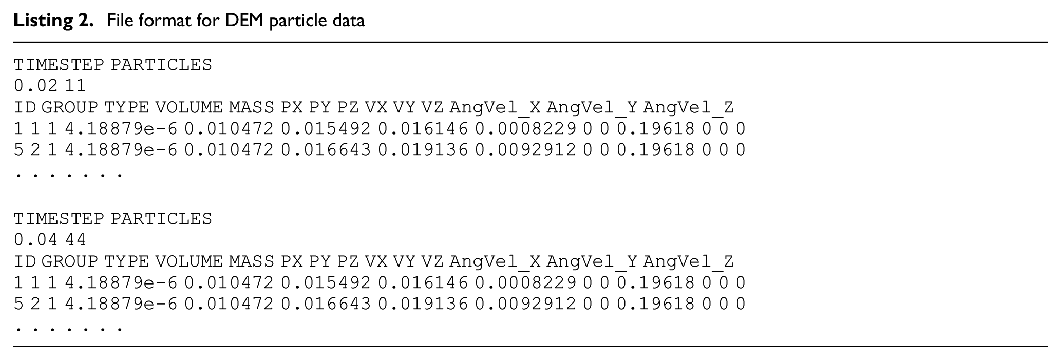
Data are provided to the platform in a file format that has been developed as an extension to ISO 10303-209:2014 Application protocol: “Multidisciplinary Analysis and Design.”35,36 A well-defined input format allows the platform to be used by many different simulation solvers with ease. An example of the standard input for DEM data for spherical particles is presented in Listing 2, which also shows how an optional variable, angular velocity (in a vector format), can be included. Additional variables can be defined as either vectors or scalars. The orientation of non-spherical particles can be accounted for by including the nine-component orientation matrix as the first additional output in the particle file.
File format for DEM particle data
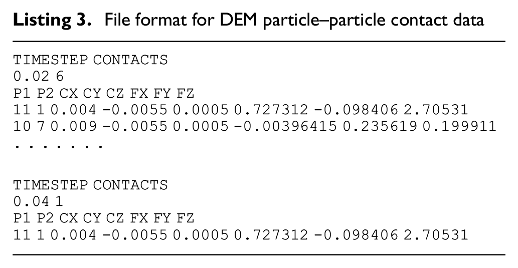
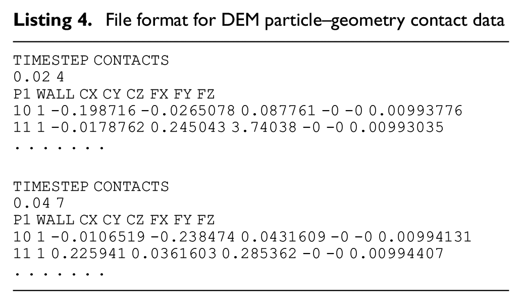
Both particle–particle and particle–geometry contact data follow the same style; examples of each file can be seen in Listings 3 and 4, respectively. Geometry meshes can be imported as standard STL files.
File format for DEM particle–particle contact data
File format for DEM particle–geometry contact data
3. Analysis of DEM simulation data with the VELaSSCo platform
The VELaSSCo platform has been designed such that using VELaSSCo for analysis of data becomes a relatively trivial task for the end-user, with the complexity of implementation hidden in the background. The user accesses the platform through a simple GUI that allows manipulation of the data using the features of the visualization client. Currently plugins have been written for the popular iFX and GiD visualization clients that allow these to work seamlessly with the VELaSSCo platform.
The Discrete2Continuum (D2C) transformation is one of the advanced analysis tools that has been incorporated within the platform. It applies temporal and spatial coarse graining methods to DEM simulation data to compute bulk quantities (such as solid fraction or stress tensors) that are projected onto a continuum field. The interface to the D2C query is presented in Figure 2. The interface displays the many options related to the transformation in an easy-to-access manner for the end-user in the form of a simple GUI.
The processing option can be divided into four main sections:
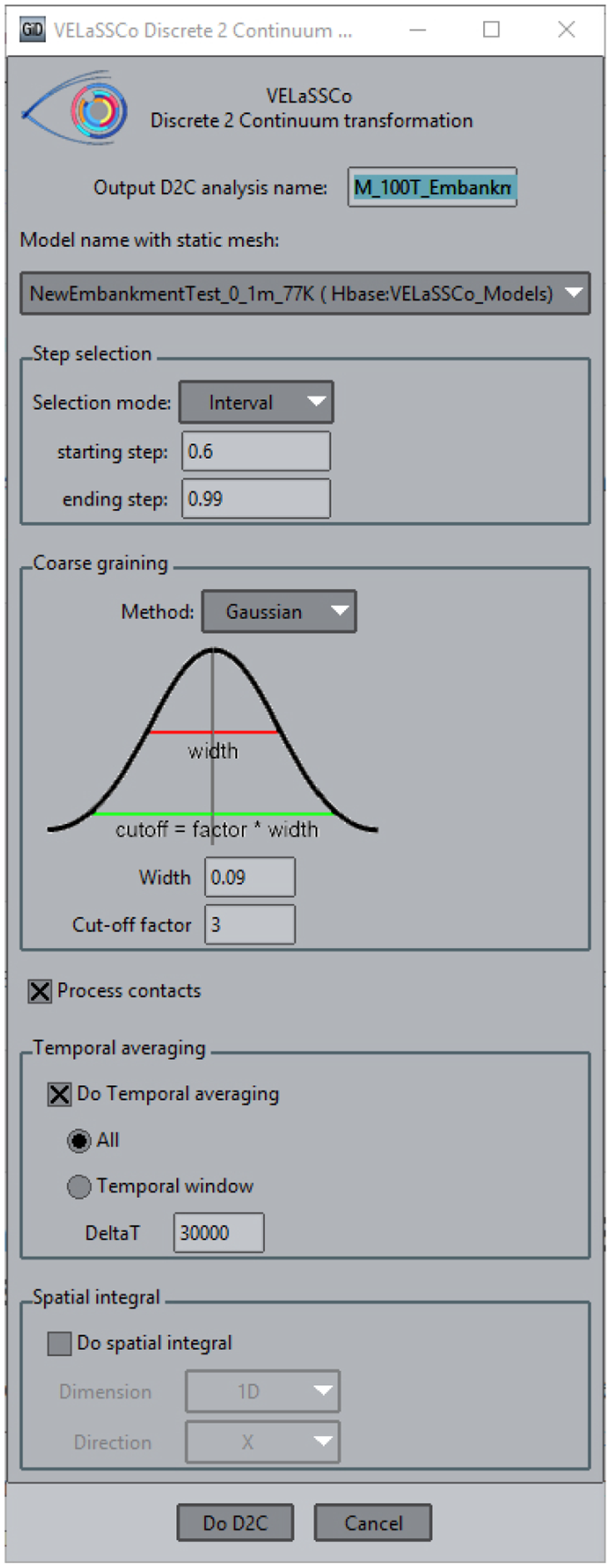
Discrete2Continuum interface on VELaSSCo.
4. Experimental setup and performance evaluation
The VELaSSCo platform is deployed on a subset of the Eddie cluster managed by the University of Edinburgh Compute and Data Facility (ECDF). The setup used for the experiments consists of 40 nodes; each node comprises two Intel Xeon CPU E5-2630@2.40 GHz (16 cores) with 64 GB of RAM and 2.8 TB of local disk storage. Without HBase replication of ingested data, this setup allows storage and processing of simulations of up to 112 TB in size. There is an additional 50 TB of network storage used to store simulation files for ingestion.
Utilizing the distributed nature of the data allows significant performance gains to be made. In particular, the default HBase replication factor ensures data blocks are distributed across multiple regions, which improves load balancing during job execution. Data for one timestep correspond to one data block. During ingestion, a distribution strategy can be specified, such as random timesteps/blocks allocated to random nodes or a range of consecutive timesteps allocated to random nodes. The latter may not be the best for parallel execution. Sometimes manual data relocation is performed to have an optimal distribution of data for a specific simulation.
The correctness of the algorithms has been thoroughly checked against a number of unit tests that take in a set of input parameters and expected outputs. The results have also been compared with those produced by other tools such as Particle Analytics software. 37 The robustness of the algorithm was tested using a fault injection strategy whereby a set of invalid input parameters or simulation data values were used to ensure that exceptional cases are handled in an appropriate manner in the algorithm without failing or creating inconsistent data in the Data Layer. For the efficiency and scalability evaluation, a set of benchmarks consisting of the two use cases described in the later sections were defined in order to assess the performance by running a number of different trials. The parameters taken into account for reproducing different benchmark test sets were the number of processors/nodes used for the computation and/or the size of the input data. Measuring the spent time of an algorithm that uses several Hadoop machines in parallel is not a trivial task. Since the input of the algorithm is stored in HBase, instead of excluding nodes from the computation by decommitting them through the editing of the configuration file in Hadoop, the number of splits of HBase regions was forced during the experiment in order to create a number of mappers equal to the number of nodes that were required for use in parallel during the experiments. For these purposes, the Hadoop JobTracker web interface visualization tool was used. The JobTracker web interface provides a wealth of information on jobs and tasks that are running on the cluster as well as historical information on completed jobs (including ones that failed). The Analyse job history link on the Job details history page displays a summary of task performance statistics and details of individual task attempts can be extracted.
The complex queries including the D2C algorithm are implemented as MapReduce jobs. The D2C is heavily optimized to run in parallel. For a given D2C process, a number of mappers are spawned across the nodes. Each mapper works simultaneously on a set of timesteps from the complete datasets to compute results associated to mesh points in the continuum field. This amounts to the top-level parallelism present in the algorithm by processing independent timesteps based on where they are located across the nodes. Further parallelization is exploited within each timestep as computation of results in the mesh can be decomposed into regions. Effectively, the D2C exploits two levels of parallelism: across nodes and within a node by leveraging multiple cores. The reduce phase performs a summary operation for, for example, computing averages and storing results back into the database.
The two levels of optimization that can be enabled during a D2C run are:
The effect of optimization level 1, which is increasing the number of nodes used to process the data, is shown in Figure 3 for the fluidized bed test case. The default optimization (single processor per node) of the D2C algorithm is tested for various sizes of simulation data (20, 40, and 100 timesteps of data). In this case, each node only processes a single timestep of data on a single processor—parallelization is achieved by distributing the timestep data across the nodes, where each node is given approximately one-third of the data for processing. The results show slightly less than linear speed-up, with a speed-up factor of 87% and measured memory ratio of 0.925 showing efficient memory usage on 1–3 nodes. Due to the problem size, as only 100 or fewer timesteps of data (with each one just over 1 MB in size) are being processed, only three nodes are used as the job setup time on each node and communication times start to become the limiting factors on performance for such a small problem.
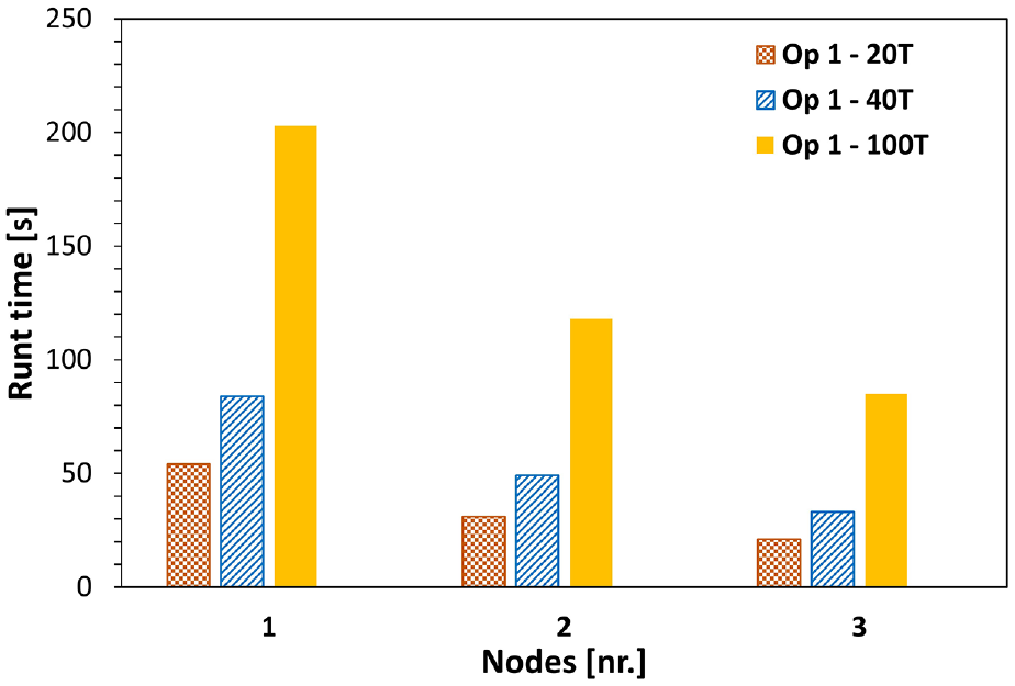
Performance benchmarks of initial discrete-to-continuum algorithm on a small dataset (fluidized bed—see Table 1 for details).
While this level of optimization shows good performance on relatively small datasets, it does not utilize the available resources fully. In order to quickly process much larger datasets, further optimization of the D2C algorithm is required to exploit all available cores on a node. At a node level, data can be further decomposed into regions and results computed in parallel using multiple processor cores available on that node (Op. 2). The increase in performance from this further optimization is illustrated by Figure 4, where the effect of node-level parallelization and node usage is shown for the large dataset. The data fall into two distinct groups based on the level of optimization used. Without node-level parallelization (Op. 1), the processing runtimes using different amounts of level 1 optimization (1, 2, and 10 nodes) are significantly higher as reflected by the three top data series. As the number of nodes utilized is increased, the total runtime begins to decrease significantly, to the point where running 10 timesteps of data across 10 nodes is only slightly slower than one timestep on one node.
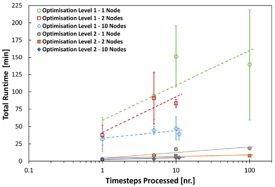
Performance of discrete-to-continuum algorithm on a large dataset (railway embankment—see Table 1 for details).
However, by enabling the second level of optimization, the algorithm effectively takes advantage of all processor cores on the node and shared memory access of the timestep being processed and consequently reduces the time it takes to compute results for all data significantly. The second parallel optimization is on average 10 times faster than the first version across the different simulations tested. Additionally, Figure 5 compiles the normalized runtime cost for both small and large datasets with level 2 optimization over increasing number of nodes showing a high
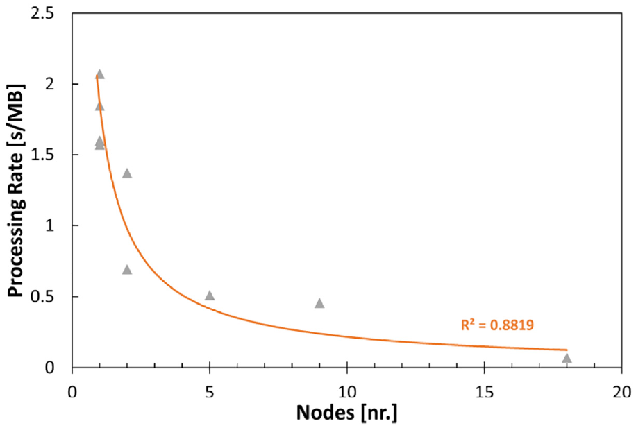
Performance of discrete-to-continuum algorithm for different-sized datasets as runtime per megabyte of data processed.
5. Sample applications and post-processed results
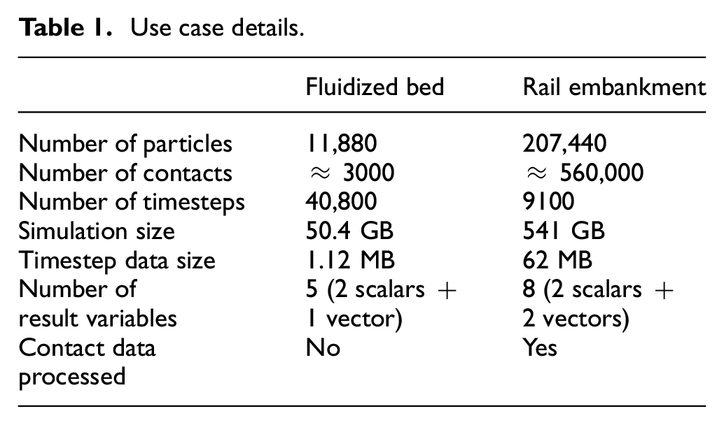
Two specific use cases (one small dataset, one large dataset) have been considered for the evaluation of the VELaSSCo platform for DEM data. The smaller dataset is for a simple fluidized bed simulation, while the large dataset is for a railway embankment simulation. The details of the use cases are presented in Table 1. Both use cases cover some of the more challenging aspects of dealing with DEM data: large amounts of particle and contact data and many timesteps.
Use case details.
5.1. Use case 1: Fluidized bed
Over the years, industries have realized that fluidized systems offer many advantages, and as a result, fluidized bed processes have become commonplace in the pharmaceutical and other chemical industries. They are able to provide high levels of contact between a solid and a gas, which makes them extremely useful as driers; fluidized bed catalytic cracking (FCC) is one of the most important and widely used refinery processes for converting low-value, heavy oils into more valuable lighter products. They are also commonly used for particle coating due to both their high gas/solid surface area and high level of mixing.
The fluidized bed use case presented here (Figure 6) is the smaller of the two use cases, although it contains data for a very large number of timesteps. Due to the dynamic nature of fluidized beds, the simulation was sampled at a high frequency, and as a result a total of 40,800 timesteps of data were generated. The results of interest in this simulation are mass, volume and velocity vector. The simulation was carried out on an HPC cluster using the MD code LAMMPS. 8
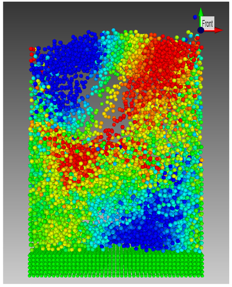
Visualized fluidized bed colored by particle vertical velocity.
Figure 6 shows a single timestep of the simulation visualized on the VELaSSCo platform using the iFX visualization client with the particle color representing the vertical velocity (
The platform provides the ability to query both the discrete particle data and the transformed continuum data. Particle-level information could be used to identify when particles experience specific zones or regimes within the bed, such as passing through a bubble or being at the free surface, by the changing velocity history. It may also be used to analyze the cyclic nature of the data and determine the frequency of any repeating phenomenon occurring in the simulation. Figure 7 shows the effect of temporal averaging on the evolution of the spatially averaged velocity magnitude for a chosen node which is at the center of a horizontal plane through the bed at approximately one-quarter bed height.
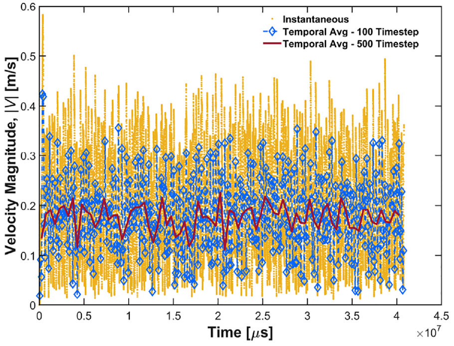
Comparison of temporally averaging window length on velocity magnitude in a fluidized bed centered on t = 20.4 s.
The combination of both spatial and temporal averaging can be more fully visualized in Figure 8, where the velocity field at a single timestep (at t = 20.4 s) is compared with the computed spatial averages for three different temporal windows: 100, 500, and 40,800 timesteps or 100 ms, 500 ms, and 40.8 s. The instantaneous result (Figure 8(a)) shows the locally averaged particle velocity at the particular instant of t = 20.4 s in the simulation. The instantaneous velocity appears significantly different to temporally averaged results at the selected timestep, with particles close to the free surface being highlighted as some of the fastest moving. The results temporally averaged over 100 ms (Figure 8(b)) show significantly reduced velocities with four “hotspot” zones. In comparison, the results temporally averaged over 500 ms (Figure 8(c)) show relatively low velocities in the upper region, suggesting that particles only intermittently enter this zone when they have a high velocity. Instead, the high-velocity zones are seen as vertical corridors pointing to a circulation pattern over the longer time frame. The final temporal window, which averages the simulation data over a much longer duration of 40.8 seconds, shows that the top of the bed typically has low particle velocities and the vertical circulation channels where high velocities are observed are now clearly visible. The similarity between the patterns observed in Figures 8(c) and 8(d) suggests that some cyclic behavior occurs in the bed, with 500 timesteps being large enough to capture at least one full cycle length.
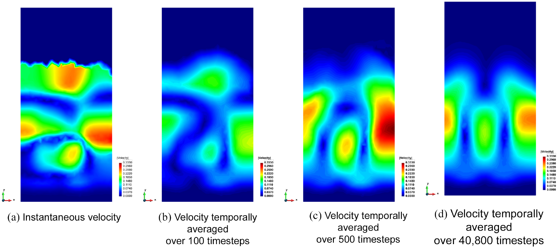
Effect of temporal averaging on the evolution of spatially averaged velocity magnitude at a fixed point in the bed for the full simulation duration.
5.2. Use case 2: Railway embankment
Significant demands are being placed on rail networks around the world, with growing traffic pushing the limits of the existing infrastructure. Extra traffic is accommodated through both higher train speeds and larger axle loads. Considering the naturally discrete, inhomogeneous structure that is a ballasted trackbed, DEM is ideally suited to study ballasted railway infrastructure. With advanced analysis tools, the stress distributions and deformation patterns that develop in ballasted track systems can be analyzed, providing key scientific insights into ballasted tracks. However, in order for the simulations to provide sufficient insight, they must be carried out on a large scale, which drives the need for a post-processing tool capable of dealing with the large volumes of data generated.
The simulation, which was carried out in the commercial code EDEM, 38 is shown in Figure 9. It produced a dataset of 540 GB for the short duration investigated. The results processed and analyzed with this dataset are mass, volume, translational and angular velocity vectors, and the contact force vector.
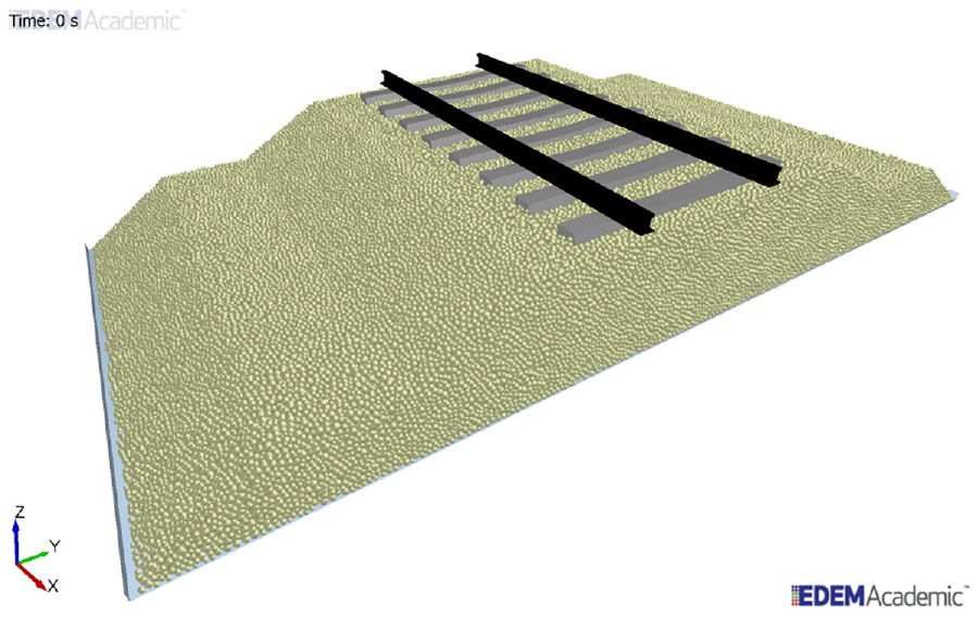
DEM simulation of a railway embankment.
The railway embankment simulations are carried out to study the effect of cyclic loading due to many trains passing, and as such are long-duration simulations that generate large amounts of data. This use case examines the effect of 10 cycles of train loading; results from the first cycle are presented here. The train is traveling from left-to-right (positive X direction) with a velocity of 70 km/h.
In Figure 10, the loading is applied by a two-axle bogey. The first axle of the bogey is just approaching the sixth sleeper while the second axle of the bogey is directly located on the second sleeper. Figure 10(a) shows the discrete velocities of every particle for a single timestep at t = 5.17 s, while Figure 10(b) shows the spatially averaged, coarse grained (Gaussian width of two particle diameters and cut-off factor of three) vertical velocity results for the same timestep. The loaded bogey (axle pair) causes some downwards velocities in its immediate vicinity; however, the largest downward velocities are seen prior to the axle arriving (sleepers 7 and 8) due to the load being transmitted to the next sleepers through the rail. The largest upward velocities are seen after the axle has passed the sleepers, such as at the first sleeper which is unloaded. The railway embankment simulations are quasistatic scenarios where particle velocities and displacements are very low, despite the large forces applied. Due to this, there are only subtle differences between the discrete particle velocities (Figure 10(a)) and the spatially averaged instantaneous velocities (Figure 10(b)), where the extreme local particle velocities, which are not representative of the bulk response, are averaged out.
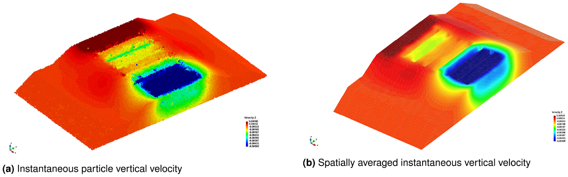
Vertical velocity in embankment at timestep t = 5.17 s.
The results in Figure 10 are only displayed on the outer skin of the 3D mesh. In order to further interrogate the data we can use the functionality of the visualization client to make several cut-planes through the 3D mesh to visualize and examine what is occurring internally in the embankment. Figure 11 shows the same vertical velocity information, but this time on cut-planes taken through the embankment at six locations: four cross-sections under the first, third, sixth, and eighth sleepers, a cross-section through the middle of the embankment and a long-section along the center line of the embankment. This allows the end-user to see the extent to which the embankment is affected internally by the loading.
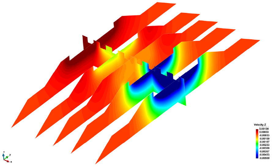
Cut-planes in railway embankment showing vertical velocity at timestep t = 5.17 s.
While contour plots are very useful for understanding the overall picture, it can be difficult to quantitatively assess these results. In Figure 12 the vertical velocity profiles at two different depths for some of the cross-sections shown in Figure 11 are plotted, allowing a simple comparison to take place at predefined locations.
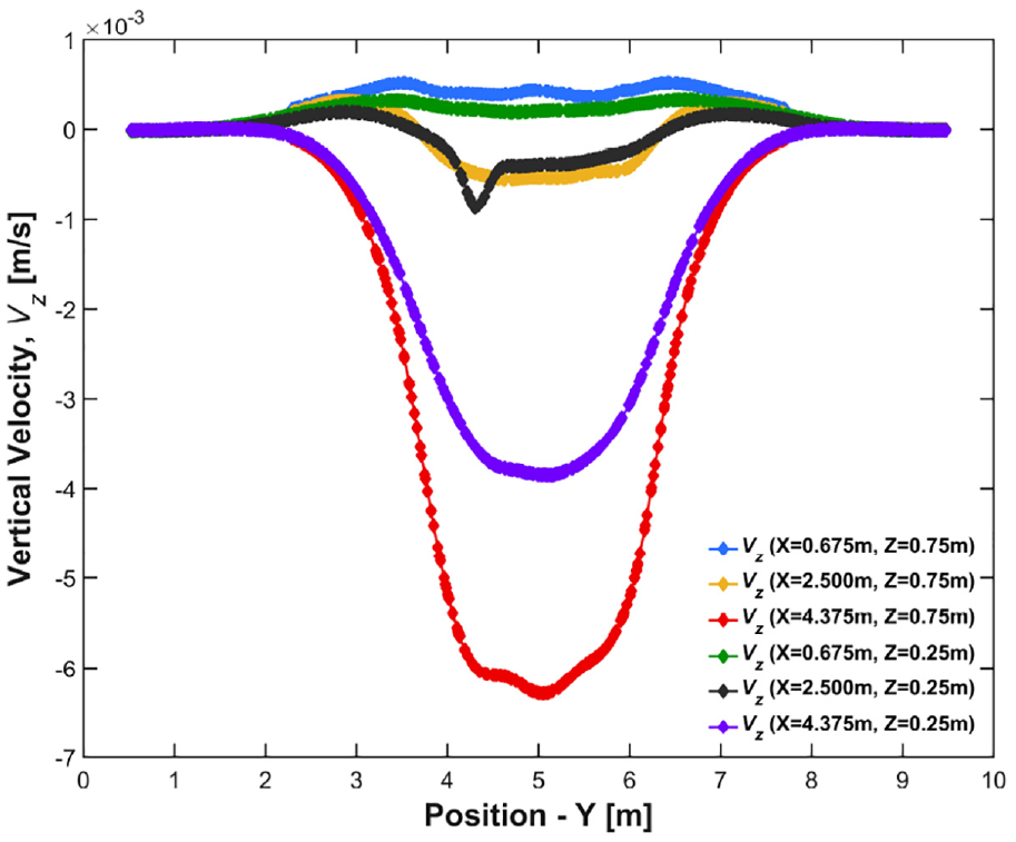
Vertical velocity profiles at two depths under sleeper 2 (X = 0.675 m), sleeper 7 (X = 4.375 m), and mid-embankment (X = 2.5 m) at timestep t = 5.17 s.
In addition to the ability to spatially and temporally average particle data, the Discrete2Continuum tool also processes contact data (where available) to compute the stress field, and other properties such as bulk density, momentum, and kinetic stress. This provides a wealth of information with which the end-user can gain insight into their simulation. The bulk density variation on three cut-planes in the embankment is shown in Figure 13. The results show a significant variation in the bulk density in the bed, which is actually quite representative of the inhomogeneous nature of a real-life embankment. This allows the end-user to investigate how the particle packing has been formed and to identify possible “soft spots” in the embankment—that is, areas in which the packing density is reduced, and hence where there is a lower bulk stiffness than the surrounding areas. When used in conjunction with the DEM output of sleeper geometry displacement, the relationship between deformation and packing arrangement can be investigated and used to explain phenomena such as excessive sleeper settlement. The grey areas in these figures represent areas where the computed density is artificially low close to the simulation boundary. This is an artifact of the averaging method employed in the analysis, as no boundary correction is currently applied for density.
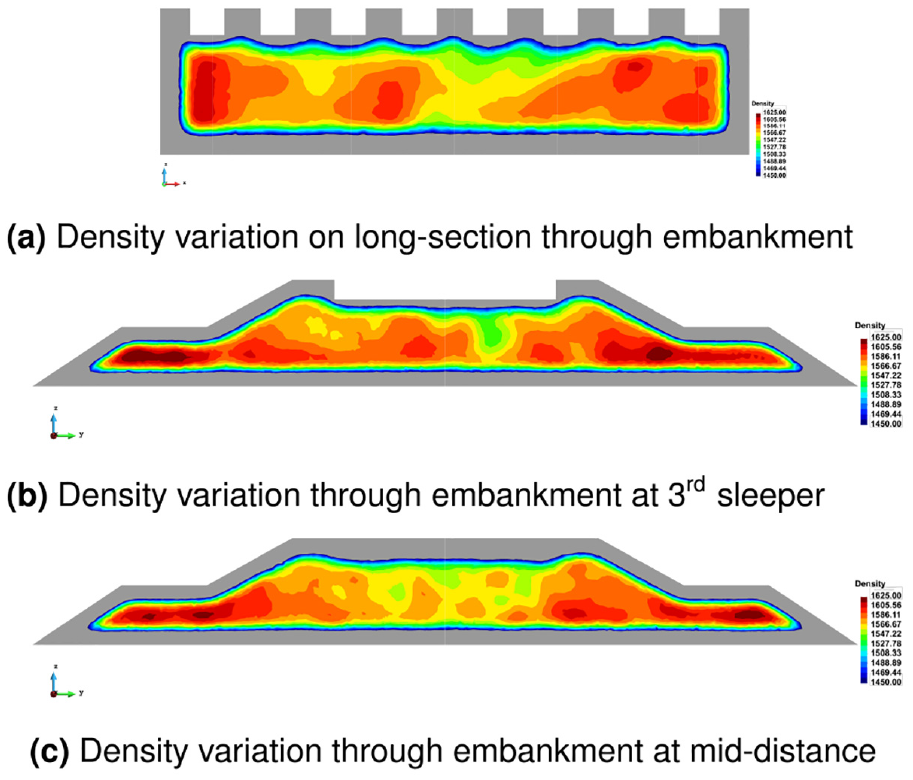
Density variation in the embankment.
The computed horizontal (
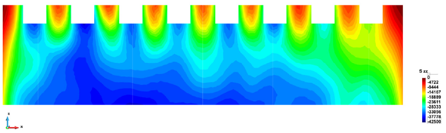
Vertical stress,
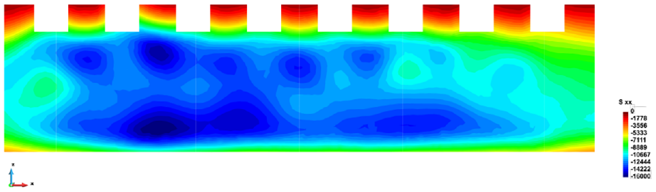
Horizontal stress,
In Figure 15 the highest longitudinal stresses,
The VELaSSCo platform has been developed to store, manage, and post-process very large simulation datasets. The results presented in the use cases so far have shown the post-processing capabilities of the platform for interrogating a single timestep of results. However, the platform also provides the ability to query the entire time range of the data, not just the currently loaded timestep. A more typical application of this capability is the creation of animations of the dataset to visualize the dynamic behavior exhibited, such as the example of a fluidized bed from use case 1. 39
Further utilizing this ability, the end-user can extract some results and see their variation over time, such as in Figure 16, where the evolution of the vertical stress in the rail embankment at three points of interest for the first loading cycle is shown. While analysis like this is trivial for small datasets and could easily be accomplished on a conventional workstation, this sort of analysis would not be possible for large datasets on such a workstation due to the limited memory, storage space, and computational power.
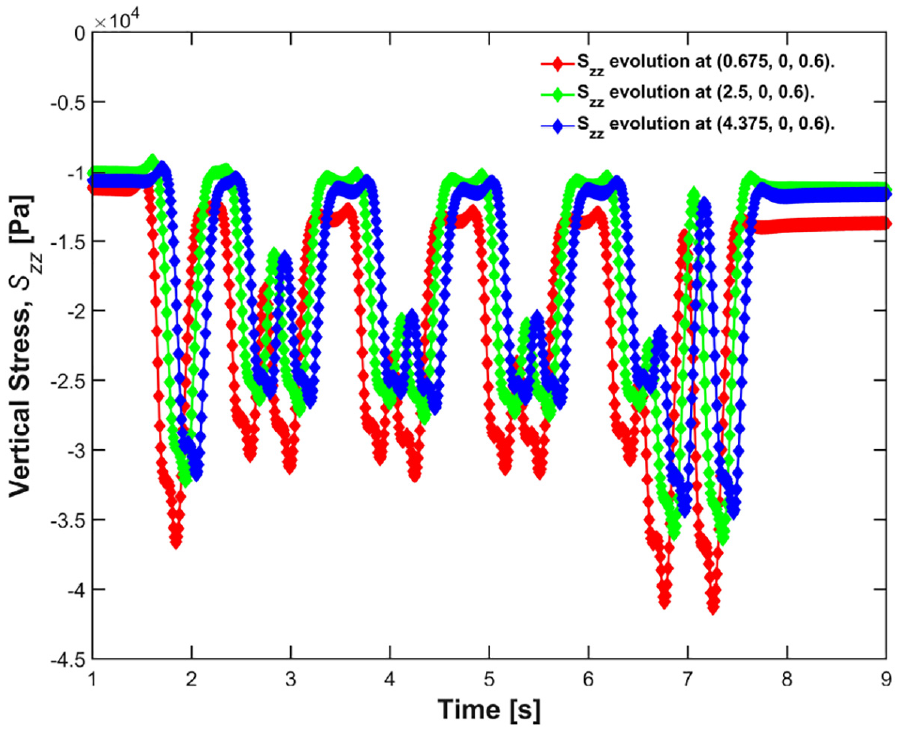
Vertical stress evolution at three locations in the embankment.
6. Conclusions
This paper has described the development of the VELaSSCo platform, which is a powerful, flexible tool for the visualization and analysis of large datasets. The platform is built on top of the open-source Hadoop software stack and utilizes the HDFS to safely and efficiently manage extremely large datasets. The architecture has been designed to allow fast processing of simulation data on the cluster before efficiently transferring the requested result back to the visualization client on the desktop. Scalability was a key consideration for the architecture and the platform can be deployed on custom clusters consisting of several hundreds or thousands of nodes, and accommodate very large distributed datasets. Key to improved performance is an effective distribution strategy of data across the nodes, and a processing algorithm adapted to take advantage of this.
There are many DEM solvers currently freely available as open-source software, as well as many other commercial codes. In order to make the platform work with such a large group of software, a file format for exporting DEM data was developed. This has been accepted as an extension to ISO 10303-209: “Multidisciplinary Analysis and Design.” 35
The Discrete2Continuum module is a tool that provides advanced analytics for DEM datasets, far beyond the simple visualization and querying of particle properties. The module is a highly optimized toolbox that can analyze the particle data across different spatial and temporal length scales and provide key macroscopic properties such as stress, density, and velocity. The distributed nature of the architecture means there is a significant performance increase for large datasets from adopting Big Data methodology for importing and storing raw data. The algorithm has been heavily optimized to run in parallel across both multiple cores on a node and multiple nodes on a cluster, which has led to significant decreases in runtime from a simple implementation, as would be common on a conventional workstation.
A selection of use cases have been presented to show the VELaSSCo platform at work. These use cases highlight datasets that are typically difficult to process on a standard workstation due to their large size and memory footprint. Using the VELaSSCo platform, these datasets can be processed in the background and then streamed back to the visualization client on the desktop for viewing of the results. The results highlight both the need to and advantage of being able to carry out such spatial and temporal averaging on DEM datasets, as the end-user is able to access revealing information that cannot be seen in the particle data alone.
Footnotes
Acknowledgements
The authors acknowledge the contribution made by the entire VELaSSCo consortium of seven partners to the development of the platform. The feedback of the user panel has been invaluable for guiding the development of VELaSSCo. This work has made use of the resources provided by the Edinburgh Compute and Data Facility (ECDF).
Funding
The development of the VELaSSCo platform was funded by the European Union’s Seventh Framework Programme (FP7/2007–2013) under Grant Agreement No. 619439.