
Abstract
With the advent of new sensor technologies and communication solutions, the availability of data for discrete event systems has greatly increased. This motivates research on data assimilation for discrete event simulations that has not yet fully matured. This paper presents a particle filter-based data assimilation framework for discrete event simulations. The framework is formally defined based on the Discrete Event System Specification formalism. To effectively apply particle filtering in discrete event simulations, we introduce an interpolation operation that considers the elapsed time (i.e., the time elapsed since the last state transition) when retrieving the model state (which was ignored in related work) in order to obtain updated state values. The data assimilation problem finally boils down to estimating the posterior distribution of a state trajectory with variable dimension. This seems to be problematic; however, it is proven that in practice we can safely apply the sequential importance sampling algorithm to update the random measure (i.e., a set of particles and their importance weights) that approximates this posterior distribution of the state trajectory with variable dimension. To illustrate the working of the proposed data assimilation framework, a case is studied in a gold mine system to estimate truck arrival times at the bottom of the vertical shaft. The results show that the framework is able to provide accurate estimation results in discrete event simulations; it is also shown that the framework is robust to errors both in the simulation model and in the data.
1 Introduction
Enabled by the increased availability of data, the data assimilation technique, 1 which incorporates measured observations into a dynamical system model to produce a time sequence of estimated system states, is gaining popularity. The main reason is that it can produce more accurate estimation results than using a single source of information from either the simulation model or the measurements. Due to this benefit, the data assimilation technique has been applied in many continuous systems applications, but very little data assimilation research has been found for discrete event simulations. With the application of new sensor technologies and communication solutions, such as smart sensors, or Internet of Things, 2 the availability of data for discrete event systems has increased as well, such as data from machines and processes, 3 or high-resolution event data in traffic. 4 The increased data availability for discrete event systems but the lack of related data assimilation techniques thus motivates this work on data assimilation in discrete event simulations.
1.1 Characteristics of discrete event simulations
Discrete event systems are usually man-made dynamic systems, for example, production or assembly lines, computer/communication networks, or traffic systems. These systems are not easily described by (partial) differential equations or difference equations; instead, they are modeled and simulated by the discrete event approach. 5 This approach abstracts the physical time and the state of the physical system as a continuous simulation time and a collection of state variables, respectively. A point on this continuous time axis at which at least one state variable changes is called instant. 6 State changes are only captured at discrete, but possibly random, instants, 7 where such a change in state occurring at an instant is called an event. 6 Since the discrete event approach jumps from one event to the next, omitting the behavior in between, it can be very efficient. 8
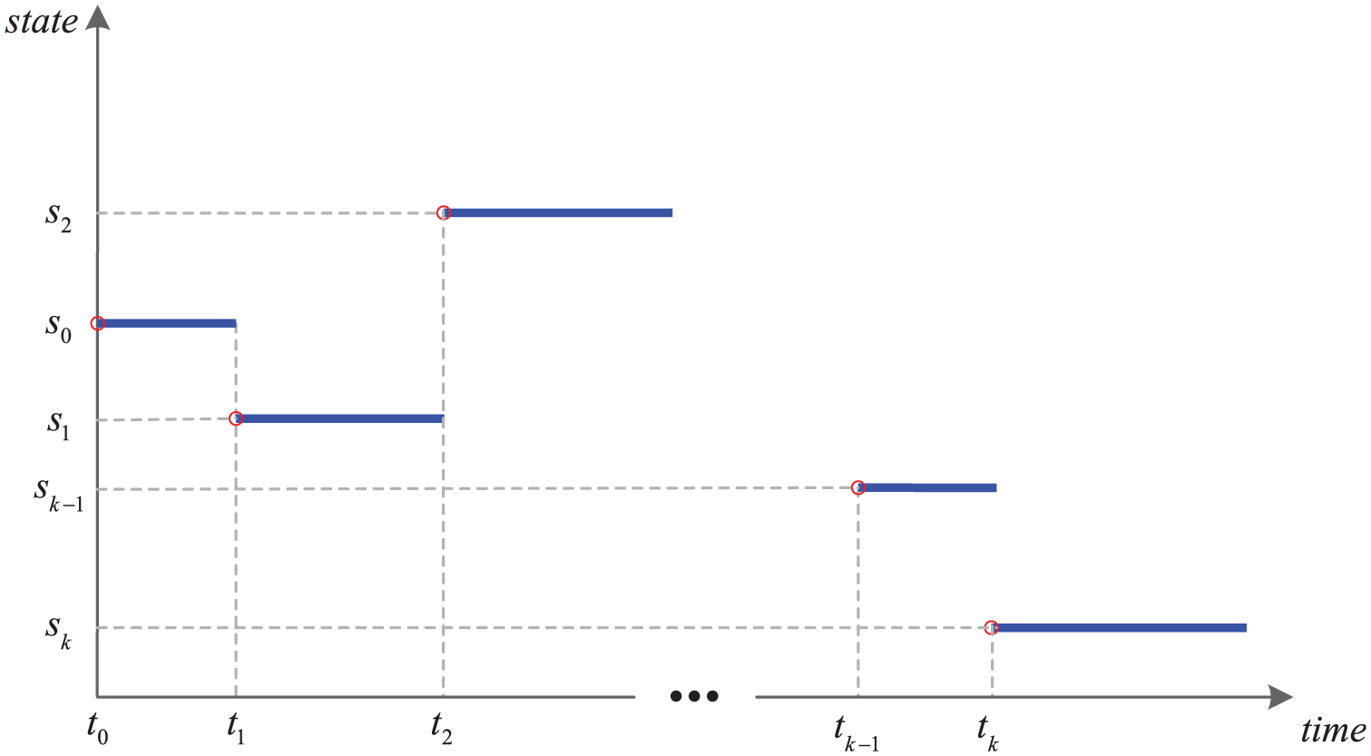
The key characteristics of discrete event simulations can be summarized as follows. Firstly, the model state is defined as a collection of atomic model states, each of which is represented by a combination of continuous and discrete variables. Take the case study in the gold mine system (see Section 3) as an example. The position of the elevator is a continuous state variable; the number of trucks that are waiting for loading is a discrete state variable; and the status of the miner, that is, busy or idle, is also a discrete state variable. Secondly, the behavior of discrete event simulations is highly nonlinear, non-Gaussian. In a discrete event simulation, the state evolution is usually based on rules, which define what the next state will be when the time advance expires, how to react when external events occur, etc. These functions are highly nonlinear step functions, because state changes in a discrete event simulation happen instantaneously at the event. The Gaussian error assumption is easily violated, since both state variables and measurements can be non-numerical. Finally, state updates in a discrete event simulation happen locally and asynchronously within each atomic model component; for each atomic model component, its state is updated at time instants lying irregularly on a continuous time axis, and the duration between two consecutive state updates is usually not fixed. The state trajectory of a discrete event simulation model is thus piecewise constant, as shown in Figure 1, which only captures changes of interest in the real state evolution.
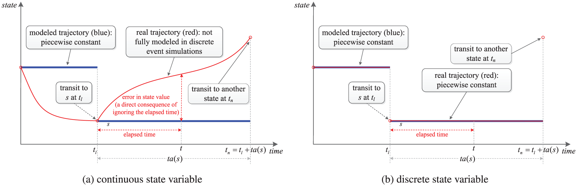
Discrete event simulation of continuous and discrete state variables. (Color online only.)
1.2 Data assimilation in discrete event simulations
The aim of data assimilation is to incorporate measured (noisy) observations into a dynamical system model in order to produce accurate estimates of all the current (and future) state variables of the system. 9 Therefore, data assimilation relies on the following three elements to work, namely the system model that describes the evolution of the state over time, the measurement model that relates noisy observations to the state, and the data assimilation techniques that carry out state estimation based on information from both the model and the measurements, and in the process address measurement and modeling errors. 1 In the literature, many data assimilation techniques exist, such as the Kalman filter, 10 the extended Kalman filter, 11 and the ensemble Kalman filter. 12 However, their working relies on certain assumptions, such as the liner model assumption or the Gaussian error assumption. 13 Another powerful data assimilation technique is particle filters.10,14 The particle filters approximate a probability density function by a set of particles and their associated importance weights, and therefore they put no assumption on the properties of the system model. As a result, they can effectively deal with nonlinear and/or non-Gaussian applications.15–17
As explained in Section 1.1, discrete event simulations are highly nonlinear, non-Gaussian systems, and therefore particle filters are in principle applicable to discrete event simulations. However, applying particle filtering in discrete event simulations still encounters several theoretical and practical problems. In discrete event simulations, state updates happen locally and asynchronously within each (atomic) model component, and the system state takes a new value when one of its components has a state update. Consequently, the time between two consecutive state updates is usually not fixed, that is, the discrete event state process is asynchronous with the measurement process, which usually feeds data at fixed times. The mismatch between the two processes incurs two problems that hinder the application of particle filtering in discrete event simulations. The first problem is the state retrieval problem, which means that the model state retrieved from a discrete event simulation model is a combination of sequential states (without the elapsed time; see Figure 1) of atomic components that were updated at past time instants. The consequence of ignoring the elapsed time is that the particles will be evaluated inaccurately, since the measurements are wrongly related to the states that were updated at past time instants. This effect is evident for continuous states (see Figure 1(a)); for discrete states (see Figure 1(b)), in order to compute the weight of a particle, one probably needs the elapsed time to define a proper measurement model that relates the discrete state to the measurement. However, ignoring the elapsed time will also make this definition and computation inaccurate. The second problem is the variable dimension problem. The “dimension” refers to the dimension of a discrete event state trajectory during a fixed time interval, which is defined as the number of state points contained in the discrete event state trajectory during that time interval. Since the duration between two consecutive state updates in a discrete event simulation is not fixed, the dimension of a discrete event state trajectory during a fixed time interval is a random variable. This will lead to inapplicability of the standard sequential importance sampling algorithm.18,19 Other practical problems, which mainly relate to data issues, such as non-numerical data, for example, event sequences, also make particle filtering in discrete event simulations highly problematic.
The research closely related to the topic of this paper is the work on data assimilation in wildfire spread simulations.15,16,20,21 However, the two problems explained above were not explicitly considered. In their work, the simulation model for wildfire spread is a cellular automaton-based discrete event simulation model called DEVS-FIRE22,23; the measurements are temperature values from sensors deployed in the fire field; particle filters are employed to assimilate these measurements into the DEVS-FIRE model to estimate the spread of the fire front. Since the measurement in the wildfire application is the temperature at a time instant, and it is only related to the system state (fire front) at the same time, their system model can be formalized as a discrete time state space model that only focuses on the state evolution at time instants when measurements are available, and the detailed evolution in between (not of interest in their application) is done with the DEVS-FIRE model. However, when retrieving the system state at the time instant when a measurement is available, the retrieved state is only a combination of sequential states of all atomic components (i.e., cells), which do not reflect any elapsed time information. As a result, errors exist, as explained in Figure 1.
1.3 Contribution and outline of this paper
In this paper, we propose a particle filter-based data assimilation framework for discrete event simulations, in which we assume that model components do not change over time (i.e., closed systems). The measurements fed at time step
The rest of this paper is organized as follows. Section 2 presents the particle filter-based data assimilation framework, which includes the system model, the measurement model, and the particle filtering algorithm for discrete event simulations. The case in the gold mine system is studied in Section 3 (tailoring the generic data assimilation framework to the specific estimation problem), Section 4 (qualitative analysis), and Section 5 (quantitative analysis). Finally, the paper is concluded in Section 6.
2 The particle filter-based data assimilation framework for discrete event simulations
In this section, the proposed data assimilation framework for discrete event simulations is presented. In order to formalize the data assimilation problem, we need to formalize the state transitions in a discrete event model as an integer indexed state process (i.e., in the same form with a discrete time model), therefore, in Section 2.1, we show how to achieve such formalization. In Section 2.2, the interpolation operation is introduced in order to obtain updated state values, and the measurement model is formalized accordingly. On the basis of the integer indexed state process and the measurement model, the particle filtering algorithm is formalized in Section 2.3, in which the variable dimension problem is addressed. Finally some practical remarks that can help simplify the application of the data assimilation framework are given in Section 2.4.
2.1 System model
In order to describe the discrete event simulations formally, we need to adopt certain discrete event modeling and simulation formalism. Therefore, in Section 2.1.1, we briefly introduce the DEVS formalism, 8 which is adopted widely in the simulation community. Subsequently, in Section 2.1.2, we introduce how the state is evolved in a DEVS model. Finally, in Section 2.1.3, we show how to formalize the state transitions in a DEVS model as an integer indexed state process.
2.1.1 Discrete Event System Specification
DEVS 8 allows for the description of system behavior at two levels: the atomic level and the coupled level. An atomic DEVS model describes the autonomous behavior of a discrete event system as a sequence of deterministic transitions between sequential states over time as well as how it reacts to external input (events) and how it generates output (events). Formally, an atomic DEVS model M is defined by the following structure:

where X and Y are the sets of input and output events, S is a set of sequential states,
Atomic models can be coupled to form a lager model. A DEVS coupled model N is defined by the following structure:

where
X and Y are the sets of input and output events of the coupled model,
D is a set of component names, and for each

for each
for each
DEVS models are closed under coupling, that is, the coupling of DEVS models defines an equivalent atomic DEVS model. 24
2.1.2 State evolution in a coupled DEVS model
Consider a coupled DEVS model N defined in Equation (1). The state evolution of its atomic component
Since DEVS models are closed under coupling,
24
the coupled DEVS model N is equivalent to an atomic DEVS model

where
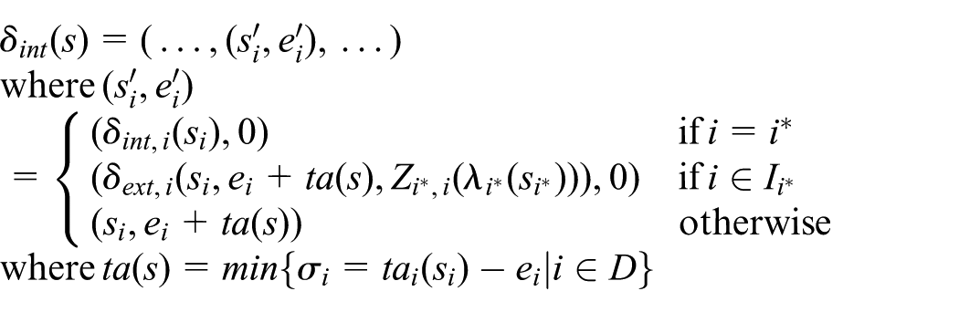
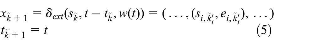
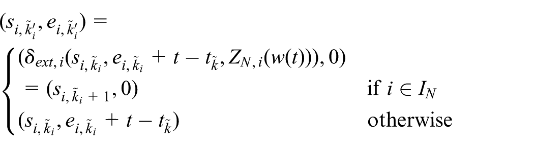
or an external state transition, which transforms the different parts of the total state as follows:
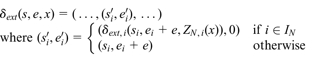
2.1.3 Formalize discrete event state evolution as an integer indexed state process
In order to formalize the data assimilation problem, we need to formalize the state transitions in a DEVS model as an integer indexed state process:
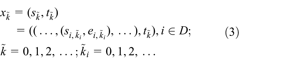
where
The integer indexed state process (each red circle represents a state point
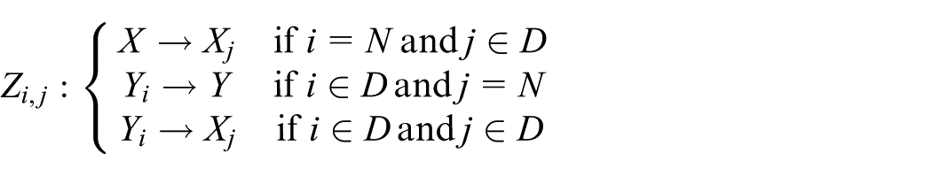
We denote the input event segment for the coupled DEVS model as
if there is no external event during
where
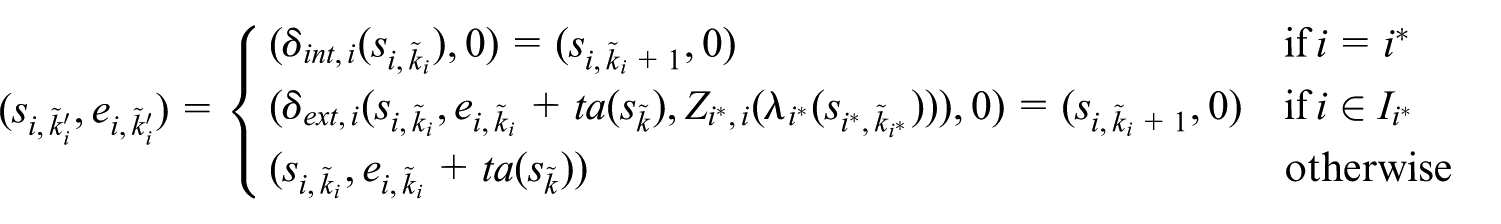
if there exist external events during
where
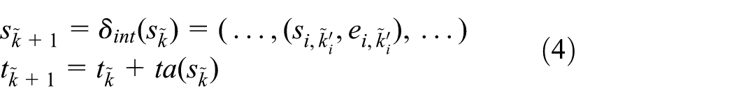
Finally, we can formalize the state evolution of a coupled DEVS model as an integer indexed state process:

where w is the input event segment and SIM is a discrete event simulation model that transfers state
2.2 Measurement model
The (discrete time) measurement model relates noisy observations to the system state:

where
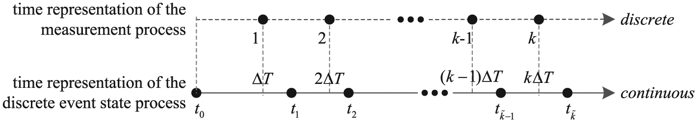
Time representation of the discrete event state process (each black dot indicates a state update) and the (discrete time) measurement process (each black dot represents the arrival of a measurement).
In a discrete event simulation, the state values are only updated when events happen. As shown in Figure 1, if we directly retrieve the model state at a time instant t, the retrieved value will be a combination of sequential states of all atomic components, which were updated at past time instants. If these retrieved states (updated at past time instants) were used for estimation, inaccurate estimation results would be obtained. This will incur the state retrieval problem, as introduced in Section 1.2. To get an updated (thus more accurate) state value at a time instant t, we need to consider the time elapsed since the model transfers to the current (sequential) state as well. Therefore, we introduce an interpolation operation to obtain the updated state value, which infers the state value at a time instant t based on the states lying around that time (i.e., neighborhood of t). How many states are involved in the interpolation is determined by the interpolation method we use. In the measurement model, the time is represented by an integer k; therefore, we define how to obtain the state value at time k (i.e.,

where

which is just a reformulation of Equation (7).
In this research, we want to generalize the measurement model to include situations where measurements are dependent on the state trajectory, that is, the history of state transitions, which means that

where
2.3 State estimation using particle filters
2.3.1 Principles of particle filters
A general discrete time state evolution can be expressed by the following:

where

where
The objective of the particle filter is to estimate the conditional distribution of all states up to time k given all available measurements up to k, that is,
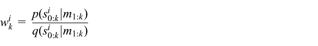
Let
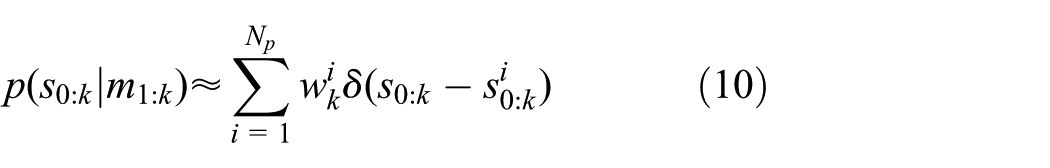
where
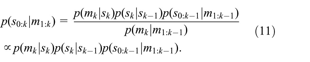
Based on Bayes’ theorem,
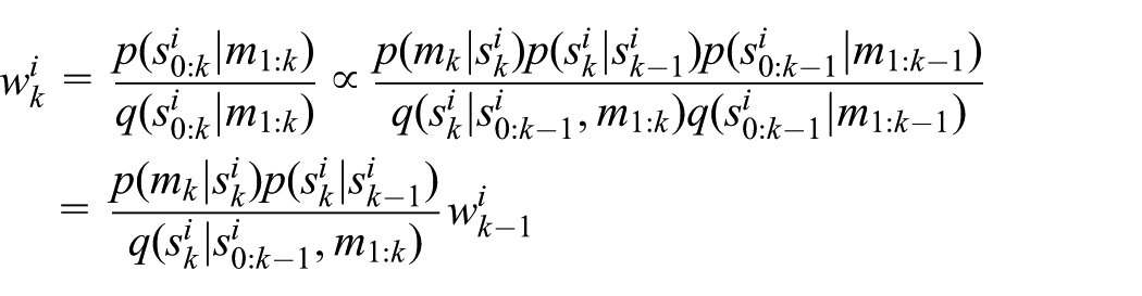
In the case that the importance density is chosen to factorize such that
obtain samples
update weights by the following:
If we assume that
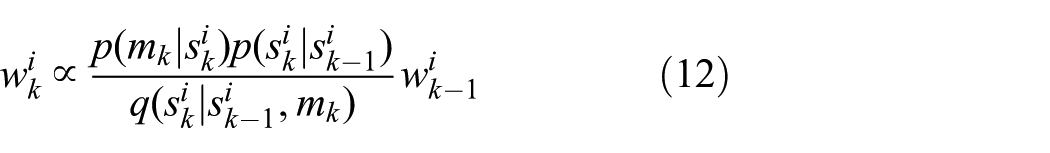
A pragmatic choice for the importance density is the system transition density, that is,

A major problem of particle filters is that the discrete random measure degenerates quickly.10,14 In other words, most particles except for a few are assigned negligible weights. The solution is to resample the particles after they are updated. Different resampling algorithms and methods exist to determine when resampling is necessary.10,14,25 A simple and often adopted resampling method is to replicate particles in proportion to their weights. It has been shown that a sufficiently large number of particles are able to converge to the true posterior distribution even in nonlinear, non-Gaussian dynamic systems.10,14
2.3.2 Application in discrete event simulations
Consider a discrete event system with sensors deployed to monitor its operation. The measurement fed at time k, that is,
Consequently, we can obtain a sequential update equation:
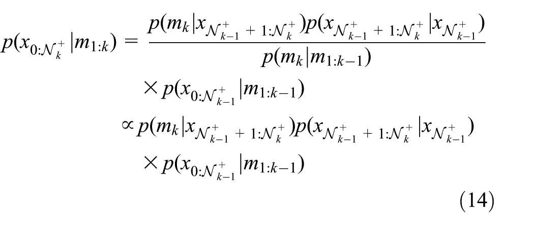
This sequential update equation is similar in form to that in Equation (11), but an important difference here is that
In Godsill et al.,
19
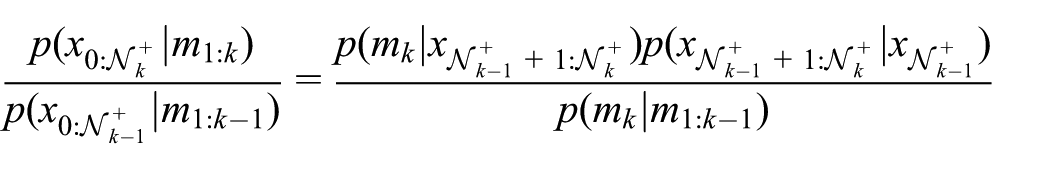
the authors proposed a solution to solve the variable dimension problem. Instead of estimating
where
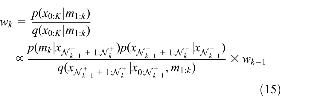
Suppose we have a large number
2.4 Practical remarks
2.4.1 The sampling procedure
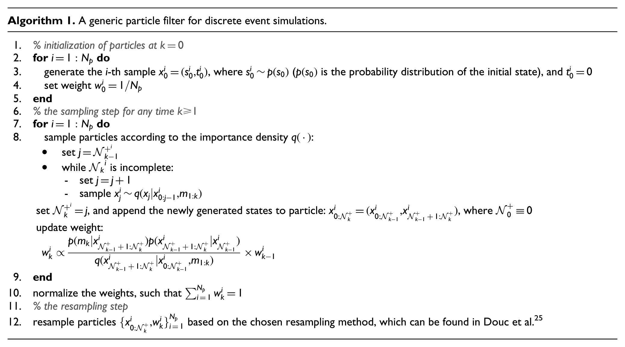
As shown in Algorithm 1, once
The two state generation processes are compared in Figure 4. The blue and red dots represent state points in a discrete event state process. Specifically, the blue dots represent state points generated in the
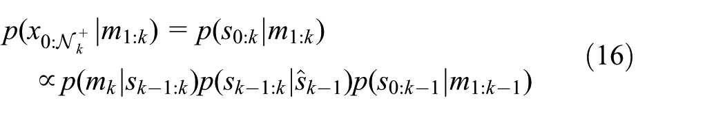
where the partial state trajectory
The weight update in Equation (15) will thus be modified to the following:
The state points generation process (the blue (generated in the
2.4.2 Generating initial particles
Generating initial particles boils down to generating initial model states. For a discrete event simulation model, we cannot generate its initial state arbitrarily (i.e., we cannot generate the initial state of each atomic model independently), since an arbitrary combination (of atomic model states) might be infeasible in reality. For example, in the gold mine case that will be studied in subsequent sections, if we generate initial states arbitrarily, we might generate a system state which indicates that the miner is drilling while no trucks are present. Therefore, initial states should be generated from a set of feasible combinations of atomic model states. Suppose the state of an atomic model can be represented as

and
Generate a feasible combination of initial phases of all atomic components,
For each atomic component - For a discrete variable in - For a continuous variable in
State variables of key components in the Discrete Event System Specification gold mine model.
Then the initial state of atomic component i can be represented as
Once we have generated the initial state
Finally, combining the generated state
3 Case study – estimating truck arrivals in a gold mine system
In this section and subsequent sections, we study a case in a gold mine system, to illustrate the working of the particle filter-based data assimilation framework introduced in Section 2. In this section, we focus on how to tailor the generic data assimilation framework to the specific estimation problem in the gold mine system.
3.1 Scenario description
A gold mine system is shown in Figure 5, and its operation is based on the coordination among miners, two trucks, and an elevator.
Miners drill at the mine shaft end, and they can only drill when an empty truck is present. Loading a truck varies very much. Creating a full truckload takes minimally 15 minutes, maximally 30 minutes.
Two trucks are available to transport ore; each truck travels 250/3 m/min when full through the mine shaft, and 500/3 m/min when empty. The current mine shaft is 400 m long.
An elevator can take a batch of gold ore up. The depth of the elevator shaft is 100 m; it takes the elevator 8 min to go up with ore and 3 min to go down empty.
When a truck is full, the miners ask the elevator to come down, so it will be at the bottom of the vertical shaft when the full truck arrives. When a truck of ore arrives at the bottom of the vertical shaft, it needs to be unloaded from the truck before the elevator can go up. Unloading takes between 5 and 10 min. After that, the elevator can go up, and the truck can go back. Unloading at the top of the vertical shaft takes between 2 and 4 min before the load can be put on a 100-m long conveyor belt that transports the gold ore to a processing plant. The conveyor belt has a speed of 10 m/min.
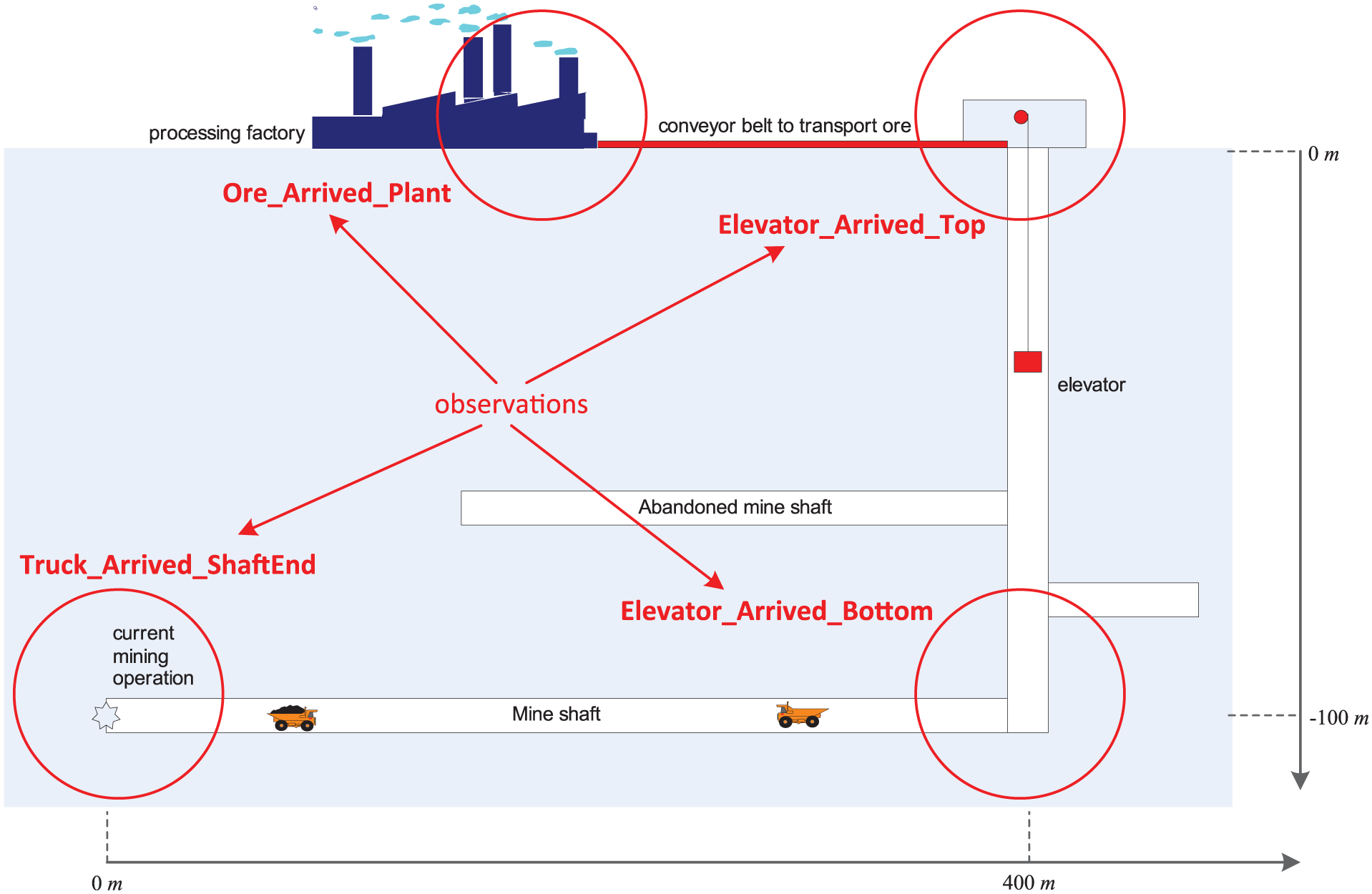
The gold mine system. (Color online only.)
The gold mine is monitored by multiple sensors, which can provide partial observations of the gold mine system (the detailed available data will be explained in Section 3.4). The problem is that, given these partial observations, can we estimate when the trucks arrive at the bottom of the vertical shaft? The arrival information is important for efficient operation of the elevator, which may improve the overall performance of the gold mine system.
3.2 Modeling the gold mine system in the DEVS formalism
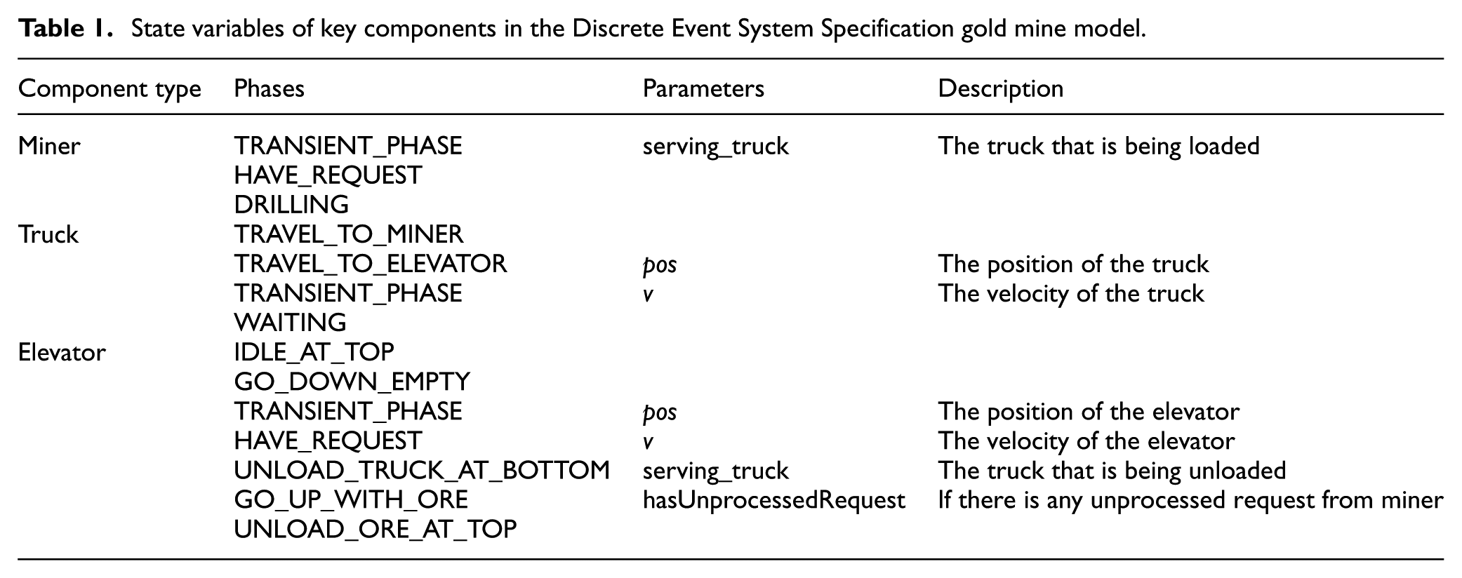
The scenario described in Section 3.1 is a typical discrete event system, and therefore we model it using the DEVS formalism, 8 as shown in Figure 6. Notice that the gold mine simulation model has no external inputs. We model each component into different phases, 26 and each phase has a name and a life time, where the name indicates the activity that the component is undergoing, and the life time tells how long the entity will stay in that phase. The phases and associated parameters (i.e., state variables) of several key components (i.e., Miner, Truck, and Elevator) are listed in Table 1, while other components (such as Queue, Conveyor, Observer) are quite simple, and therefore we do not describe them in detail due to space limitations.
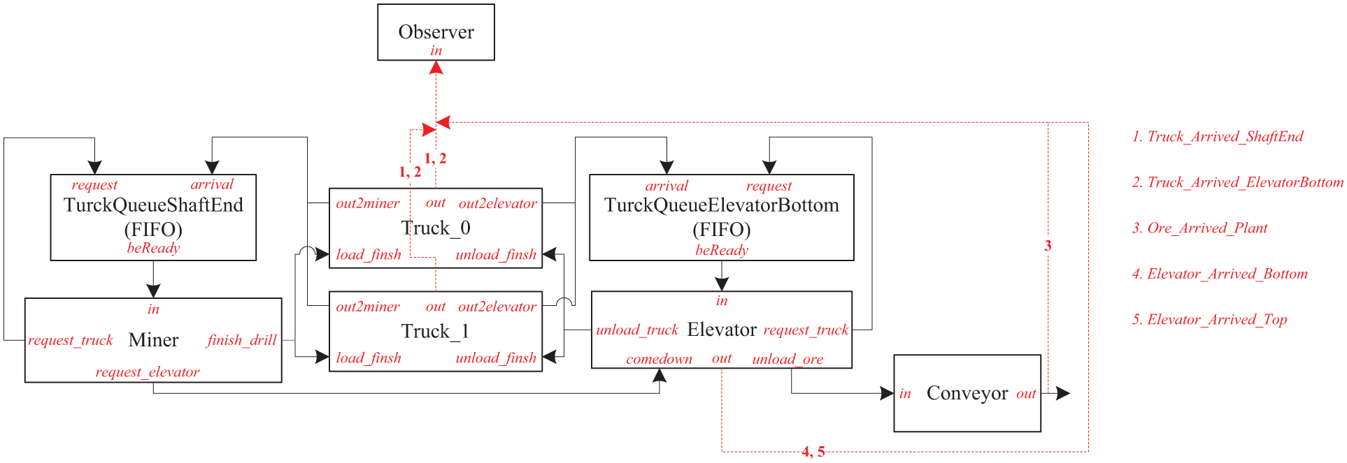
The Discrete Event System Specification model of the gold mine system. FIFO: first-in, first-out. (Color online only.)
As shown in Table 1, each component has a transient phase, that is, TRANSIENT_PHASE, which has zero length of life time and is used to request resources or jobs. For example, when Miner finishes drilling and loading, it will first make a transition from DRILLING to TRANSIENT_PHASE; since TRANSIENT_PHASE has zero length of life time, a message is immediately sent to TruckQueueShaftEnd to say that Miner is idle and can drill and load other trucks if there are any; then Miner transfers to HAVE_REQUEST (i.e., idle) to wait for new trucks. Truck and Elevator work in a similar way. The movement of the elevator and the trucks is assumed with constant speed (although not realistic).
The unloading times at the bottom and the top of the vertical shaft are modeled as Uniform distribution
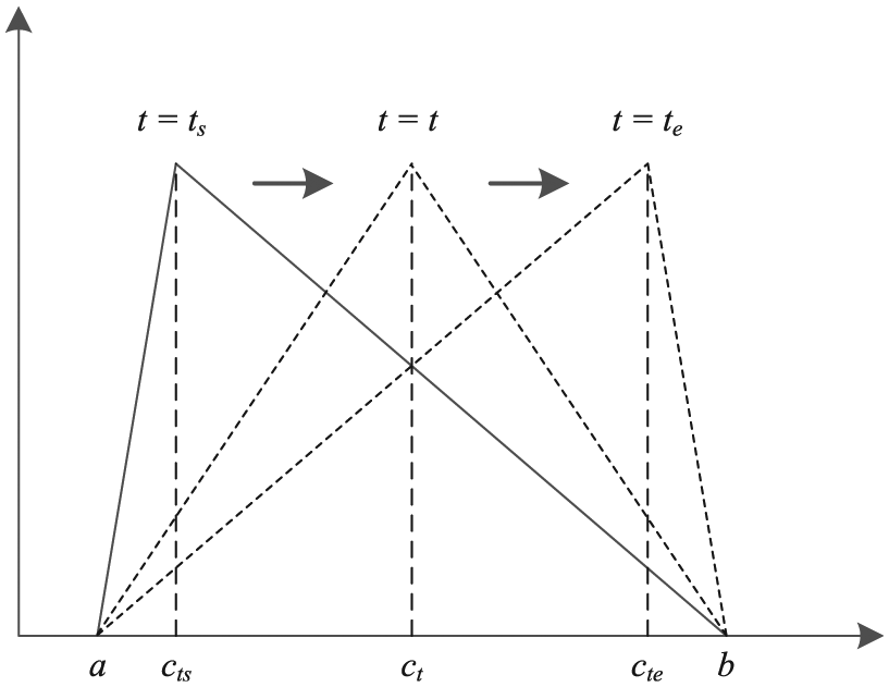
Triangular distribution with varying modes.
We denote the set of component names as D = {TruckQueueShaftEnd, TruckQueueElevatorBottom, Miner, Truck_0, Truck_1, Elevator, Conveyor, Observer}. For any component

where
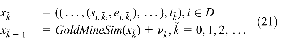
where GoldMineSim is the (discrete event) gold mine simulation model and
3.3 Interpolation operation
In this section, we introduce the interpolation method used in our gold mine case, and show the difference between the simulated state trajectory and the interpolated state trajectory. Considering that discrete state variables cannot be interpolated, we distinguish continuous states from discrete states as shown in Figure 1.
3.3.1 Continuous state
Continuous states can be interpolated. We take the elevator as an example, whose (sequential) state is represented as
As introduced in Section 3.2, the elevator moves with constant speed. Therefore, we use linear interpolation to update the elevator’s state. Suppose that the last state update was at time
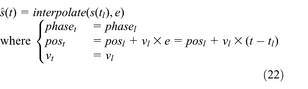
which is independent of the states beyond time t.
3.3.2 Discrete state
Discrete states cannot be interpolated. For example, the (sequential) state of the miner is

where the elapsed time
3.3.3 Interpolated state
Suppose that the (sequential) state of the coupled model at time instant
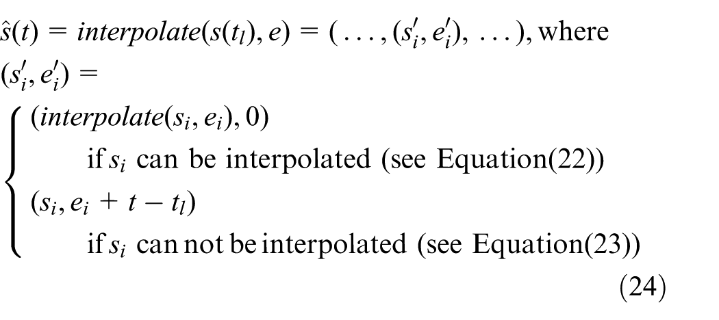
Notice that the time advance of state
3.3.4 Simulated state trajectory versus interpolated state trajectory
In this section, we show the difference between the simulated state trajectory and the interpolated state trajectory. We take the state of the elevator in terms of position as an example. As shown in Figure 8, the positions of the elevator in the discrete event simulation are captured in blue, while the interpolated state trajectory is depicted in red. Since states only change when events occur, the simulated state trajectory of the elevator in terms of position is a piecewise constant curve, while the interpolated state trajectory is a piecewise linear curve since the velocity is constant and we adopt the liner interpolation method. Note that the piecewise constant segments between the elevator top and the elevator bottom in Figure 8 are the result of the elevator processing external events, for example, miners ask the elevator to come down.
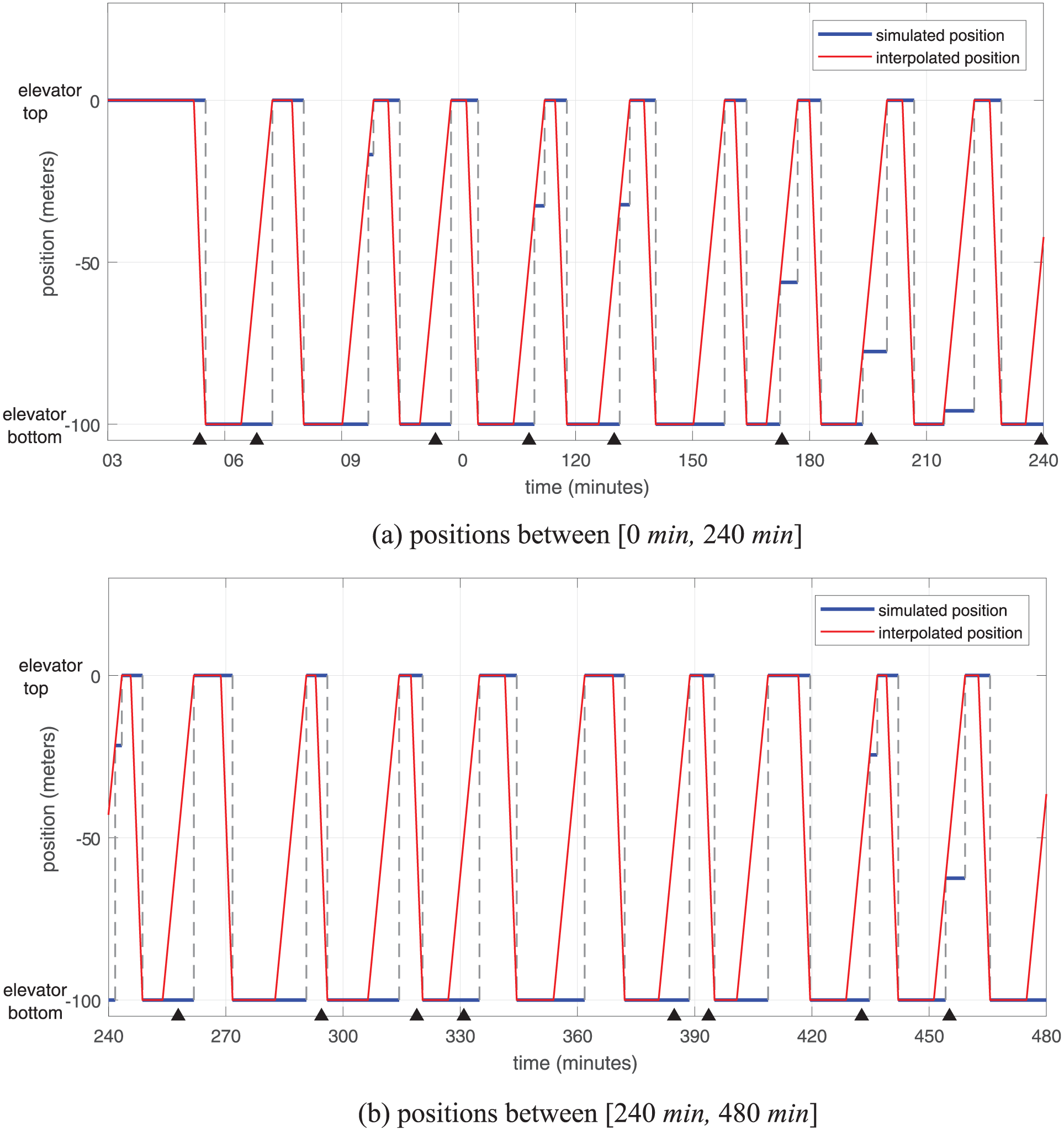
The state trajectory of the elevator in terms of position (the piecewise constant segments between the elevator top and the elevator bottom are the result of the elevator processing external events; each black triangle represents a time instant when a noisy observation of the elevator position is available; color online only).
As explained in the previous section, the elevator moves with constant speed. Therefore, the true state trajectory of the elevator in terms of position is also a piecewise linear curve, which overlaps the interpolated state trajectory. In this specific case, the resulted state trajectory by interpolation is equivalent to that if we simulate the continuous state variable (the position of the elevator) using Generalized Discrete Event Specification (GDEVS) 27 with the degree of the polynomial equal to 1. Notice that if the elevator has a different speed profile, for example, accelerate–constant speed–decelerate, the true state trajectory in terms of position and the interpolated state trajectory will not overlap any more. From Figure 8, we can clearly see that if we retrieve the state of a discrete event simulation model without interpolation, the retrieved state is only a past state that was updated at a past time instant, which cannot reflect real-time evolutions of the state; therefore, errors would be incurred if the outdated states are used for estimation. This will be proven in Section 5.
3.4 Available data and measurement model
The simulated data is generated by running the gold mine simulation (Section 3.2) for 480 min. During the run, all events are recorded; the states of the elevator and the trucks are sampled (using interpolation) and recorded very densely (every 0.01 min) in order to obtain their detailed evolutions; the data recorded for the elevator and the trucks includes phase names and their real-time positions. This ground-truth data is then processed as follows.
We extract the event sequence that only contains the following types of events (as shown in Figure 5): trucks arriving at the shaft end (Truck_Arrived_ShaftEnd); the elevator arriving at the top or the bottom of the vertical shaft (Elevator_Arrived_Top, Elevator_Arrived_Bottom); and a batch of ore arriving at the plant (Ore_Arrived_Plant). This event sequence is partial, but accurate (i.e., no missed events, and occurrence times are accurate).
We add Gaussian noise to the positions of the elevator and the trucks, respectively; specifically, we add noise drawn from
The noisy dataset is used for data assimilation, and we set the measurement interval to
Event sequence
To summarize, the measurement available at time k can be represented as follows:

and the measurement model can be formalized as follows:

where

where
3.5 Estimating truck arrivals using particle filters
Having formalized the system model (Section 3.2) and the measurement model (Section 3.4), in this section, we implement (on the algorithmic level) the particle filtering framework (Section 2) in the (discrete event) gold mine simulation to illustrate the working of the framework by estimating the truck arrivals at the bottom of the vertical shaft.
3.5.1 Particle filtering for truck arrivals estimation
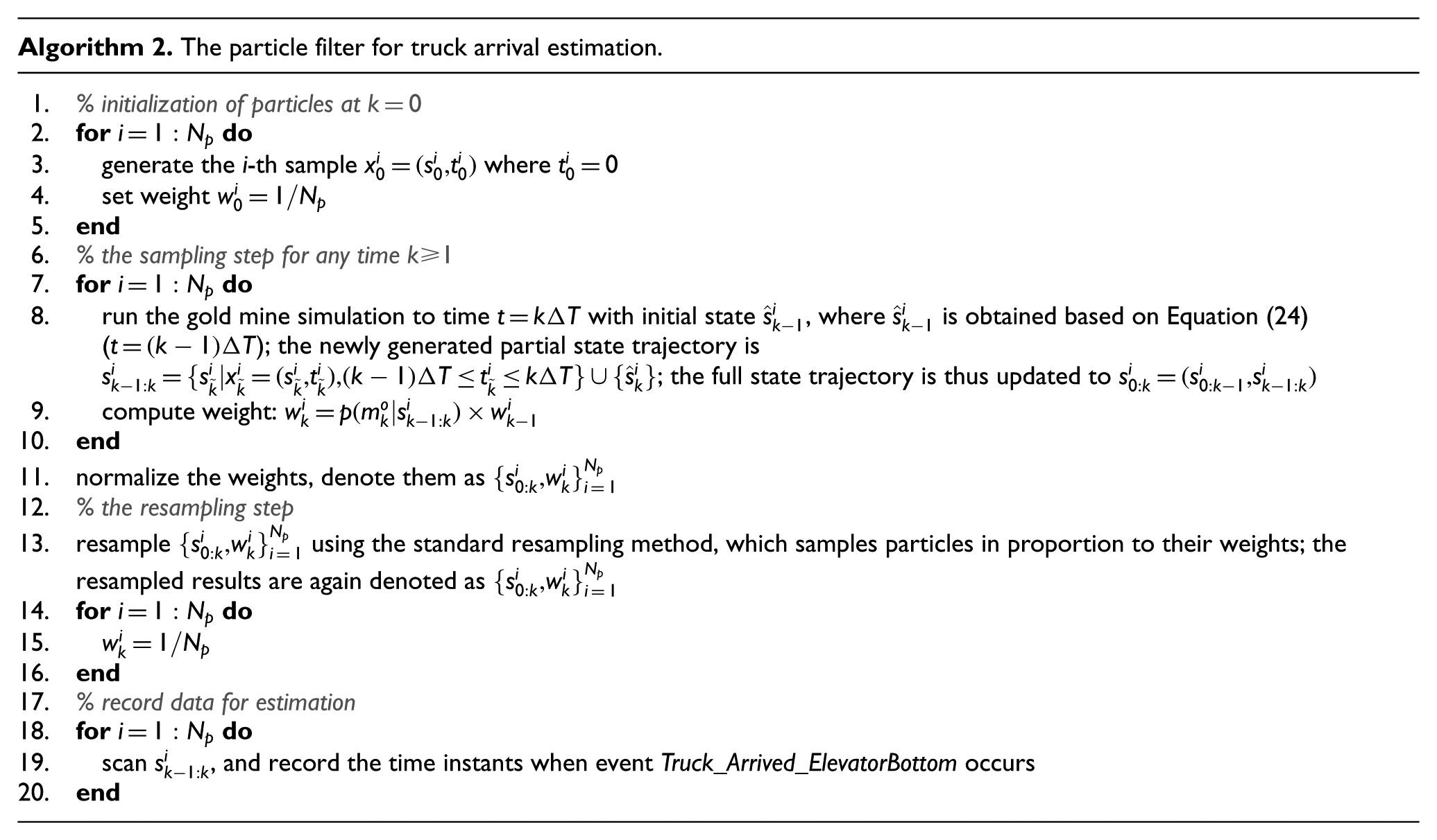
Algorithm 2 describes in detail how the generic particle filter shown in Algorithm 1 is applied in the specific gold mine case to fulfill the truck arrival estimation task. Since the interpolation operation at any time instant t is independent of states beyond that time, the formalization of Algorithm 2 is focused on system states
3.5.2 Generating initial particles
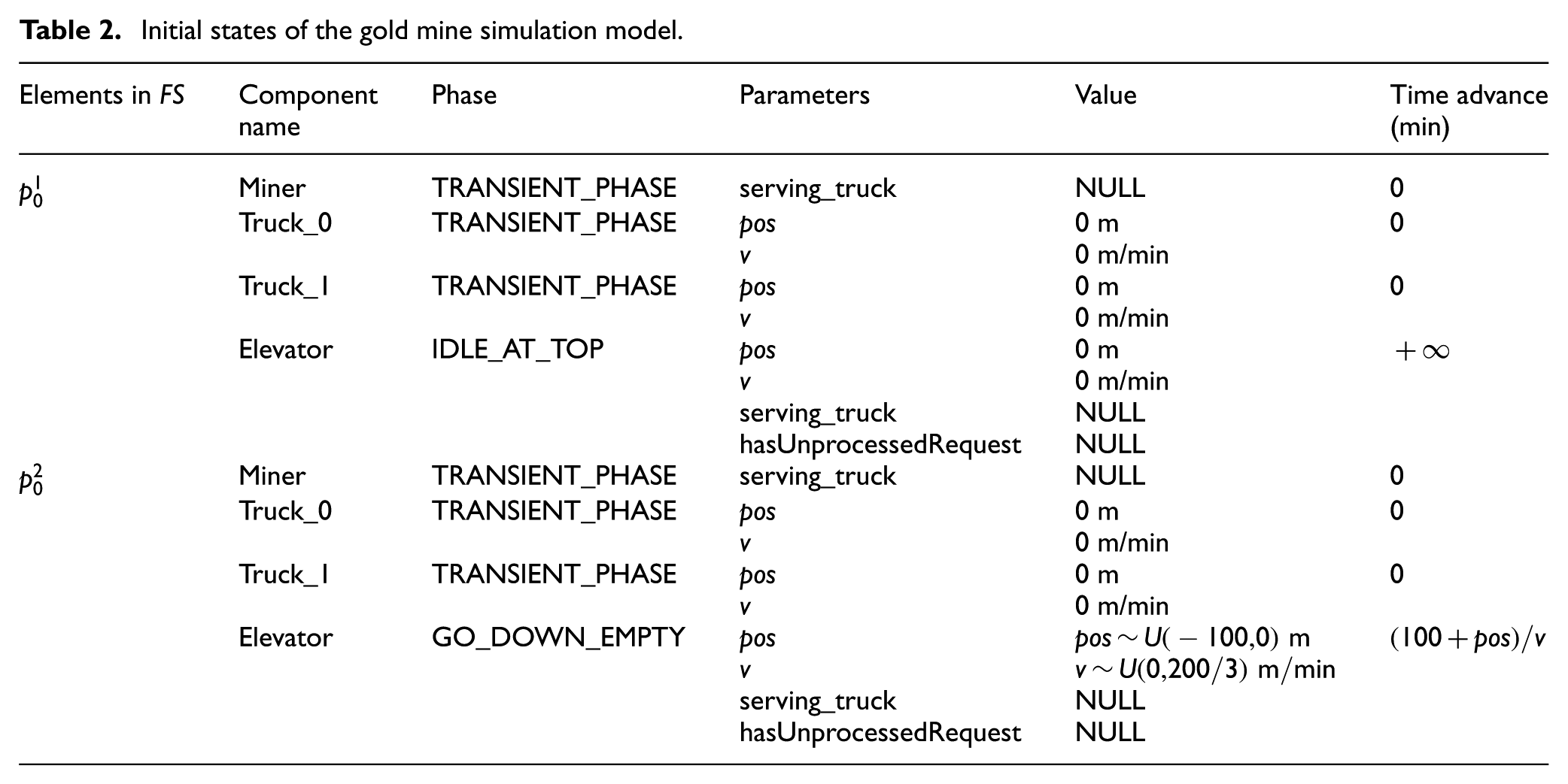
In this case study, initial particles are generated based on the procedure introduced in Section 2.4.2. For illustration purpose, we only enumerate two feasible combinations of phases, which are listed in Table 2, although there are many more feasible choices. We assume
Initial states of the gold mine simulation model.
3.5.3 Weight computation
In this section, we detail how the weight is computed, that is, we utilize
3.5.3.1 Event sequences
Given state points
An event can be modeled as a two-tuple

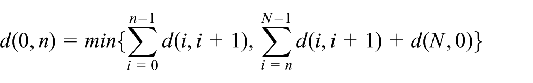
We adopt the edit distance
28
to define the “distance” between two event sequences. The edit distance is defined as “the amount of work that has to be done to convert one sequence to another,” and the amount of work is quantified by a set of transformation operations and their associated costs (more details can be found in Mannila and Ronkainen
28
). Suppose
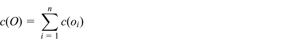
then the edit distance between event sequence S and event sequence T is defined as the minimum cost that is needed to transform S to T, that is:

where
Once the distance between two event sequences can be computed, we can now define
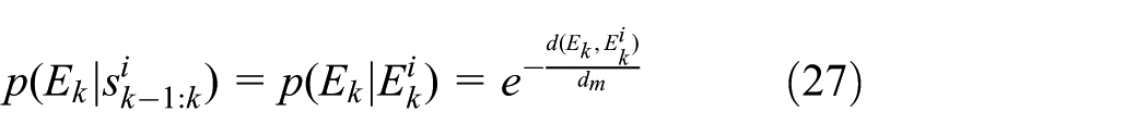
where
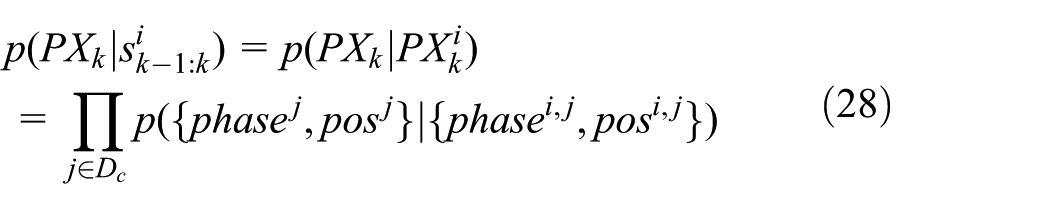
3.5.3.2 Phases and positions
Given state points
For phase and position data, we need to consider them as a whole. For example, we assume that the observation from the elevator is
The phase match method works as follows. Suppose the phase is represented as
where
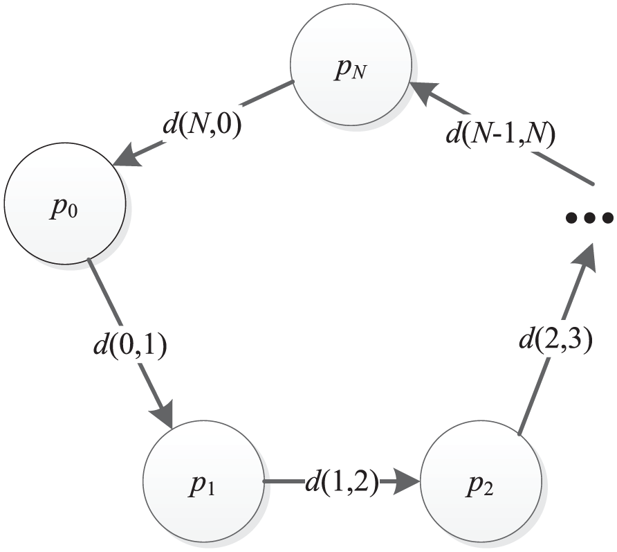
The phase transition graph.
In our case, the parameter is the position with Gaussian noise, and therefore we define
where
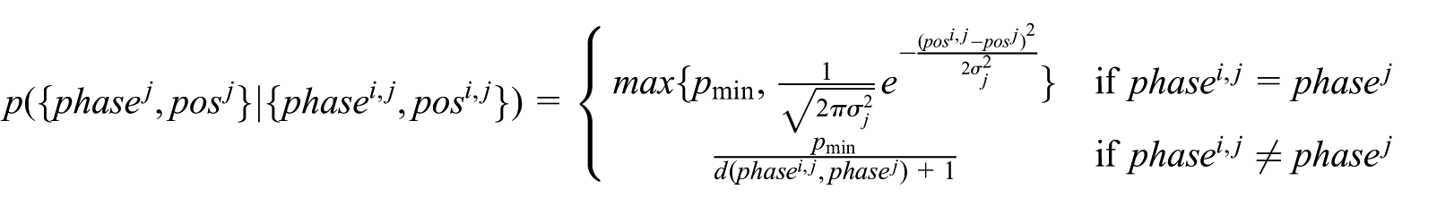
We argue that the weight of a particle in which the phase is the same as the observed phase (i.e.,
4 Case study of the gold mine system – qualitative analysis
In this section, a qualitative analysis is conducted to compare the estimation results without and with assimilating noisy observations; the objective of this comparison is to prove the necessity to assimilate observations into discrete event simulations in order to get better estimation results.
If we do not assimilate noisy observations, we can run the simulation multiple times with different random seeds to generate data for estimation. Therefore, we run the gold mine simulation 2000 times with different random seeds and record the time instants when trucks arrive at the bottom of the vertical shaft. The estimation results are shown in Figure 10(a). The results show that if there is no real-time data from the real system assimilated, the discrepancy between the simulation and the real system will become larger and larger as time advances. Consequently, the simulation without data assimilation will gradually lose its prediction ability. Based on our example, from
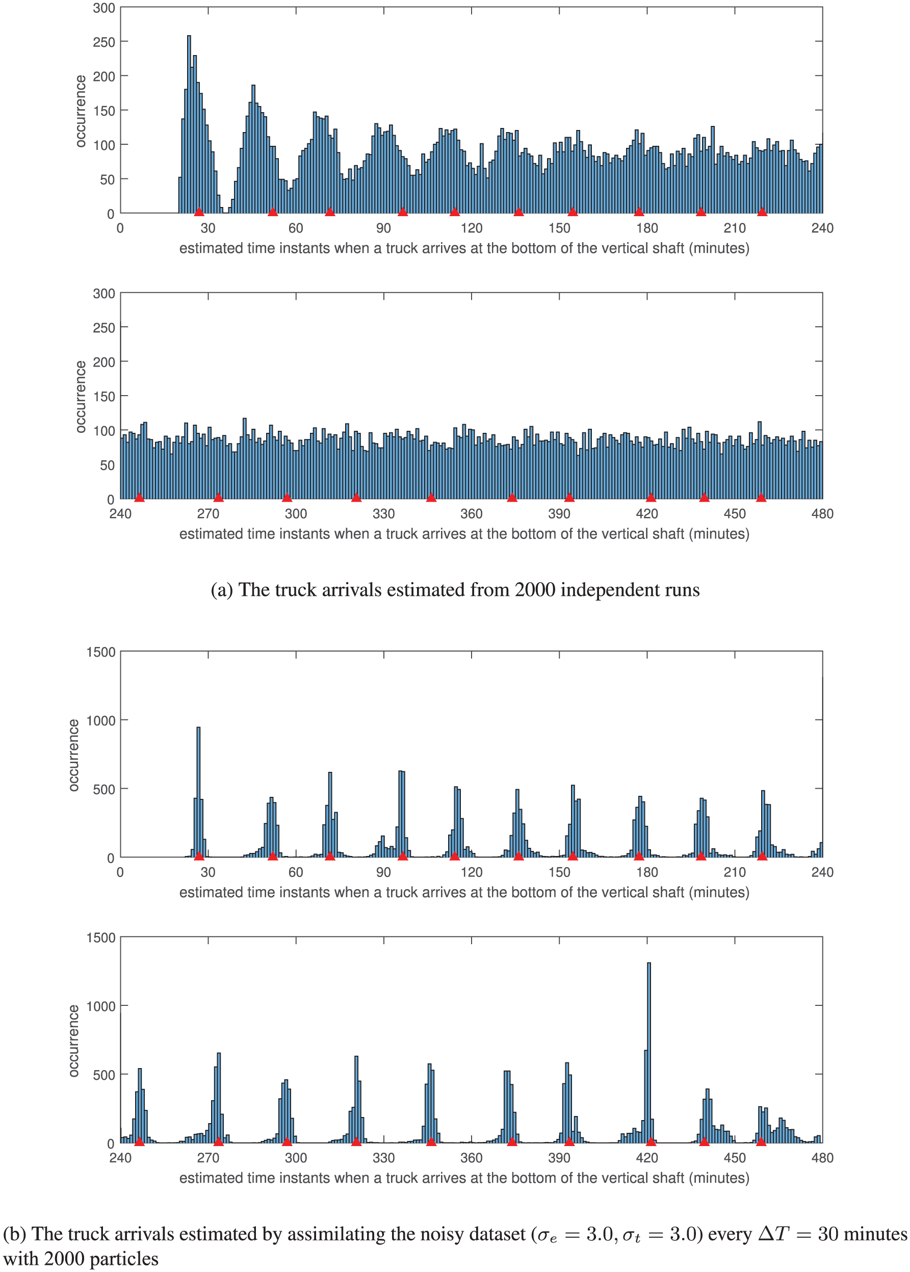
A general view of the estimation results of truck arrivals at the bottom of the vertical shaft with and without assimilating noisy data (each red triangle represents a truck arrival in ground truth; color online only).
In contrast, we use the same simulation model to assimilate the noisy dataset (
We present the estimation results of truck arrival times at the bottom of the vertical shaft in one time step (i.e.,
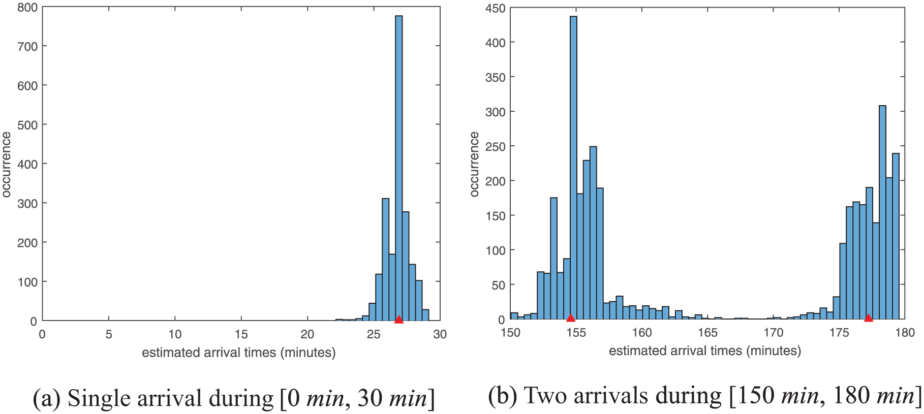
Histogram of estimated truck arrival times at the bottom of the vertical shaft during one step
5 Case study of the gold mine system – quantitative analysis
The particle filtering method shown in Algorithm 2 gives us raw estimation results of truck arrivals, which are depicted in Figure 10(b). In this section, we show how these raw data are processed in order to conduct a more informative analysis; based on the processed data, a set of performance indicators is proposed to quantify how accurate the estimation results are; finally, the results computed based on these performance indicators are presented and analyzed.
5.1 Data processing for estimating truck arrival times
As shown in Figure 11(b), the estimated truck arrival times obviously belong to two groups, each of which approximates the distribution of a truck arrival. Therefore, we cluster the estimated arrival times into groups (for example, using the k-means clustering algorithm
29
), and each group estimates one truck arrival. Suppose that there are m such clusters:
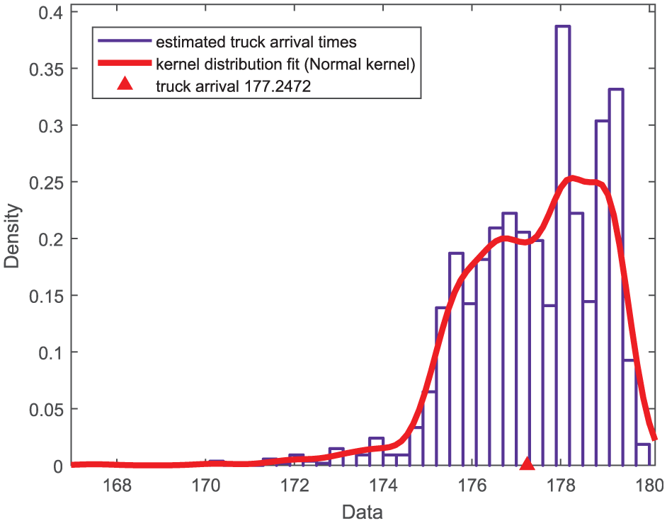
Fitting a kernel probability distribution using the Normal kernel to truck arrival times in one cluster (this group of data belongs to the cluster on the right-hand side in Figure 11(b); the red triangle represents a truck arrival in ground truth; color online only).
If we denote the fitted probability distribution from data in cluster

and for convenience, we denote this probability as
5.2 Evaluation criteria
Assume that the ground-truth value of truck arrivals is
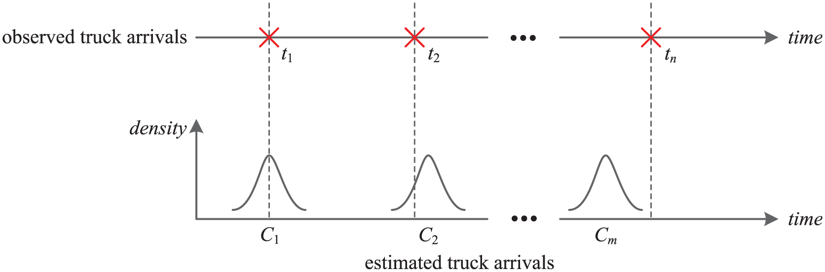
Format of the ground-truth data and estimated data. (Color online only.)
For each arrival
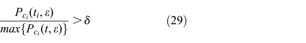
we consider that the arrival
Obviously, the more arrivals in A being successfully estimated, the better performance of the estimation. Thus, we define the success rate as follows:
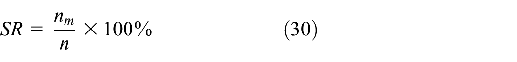
where
If a cluster
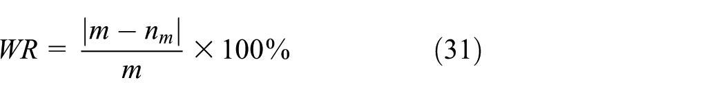
The best value of WR is
Suppose that
Average distance to the time instant when the probability density function is peaked:
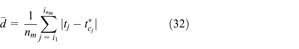
where
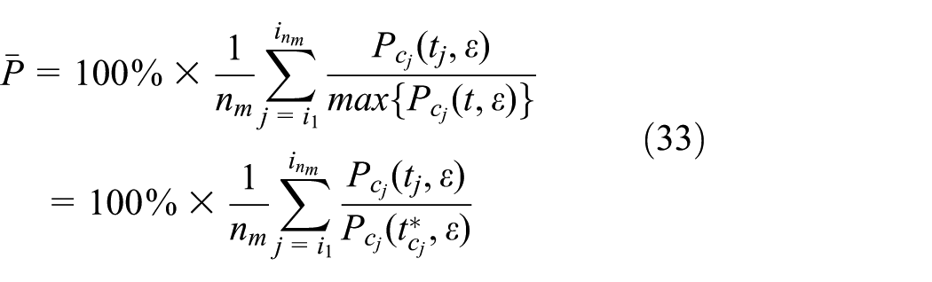
Average percentage that
5.3 Results
In this section, we present the estimation results of assimilating the noisy dataset (
5.3.1 The estimated truck arrival times
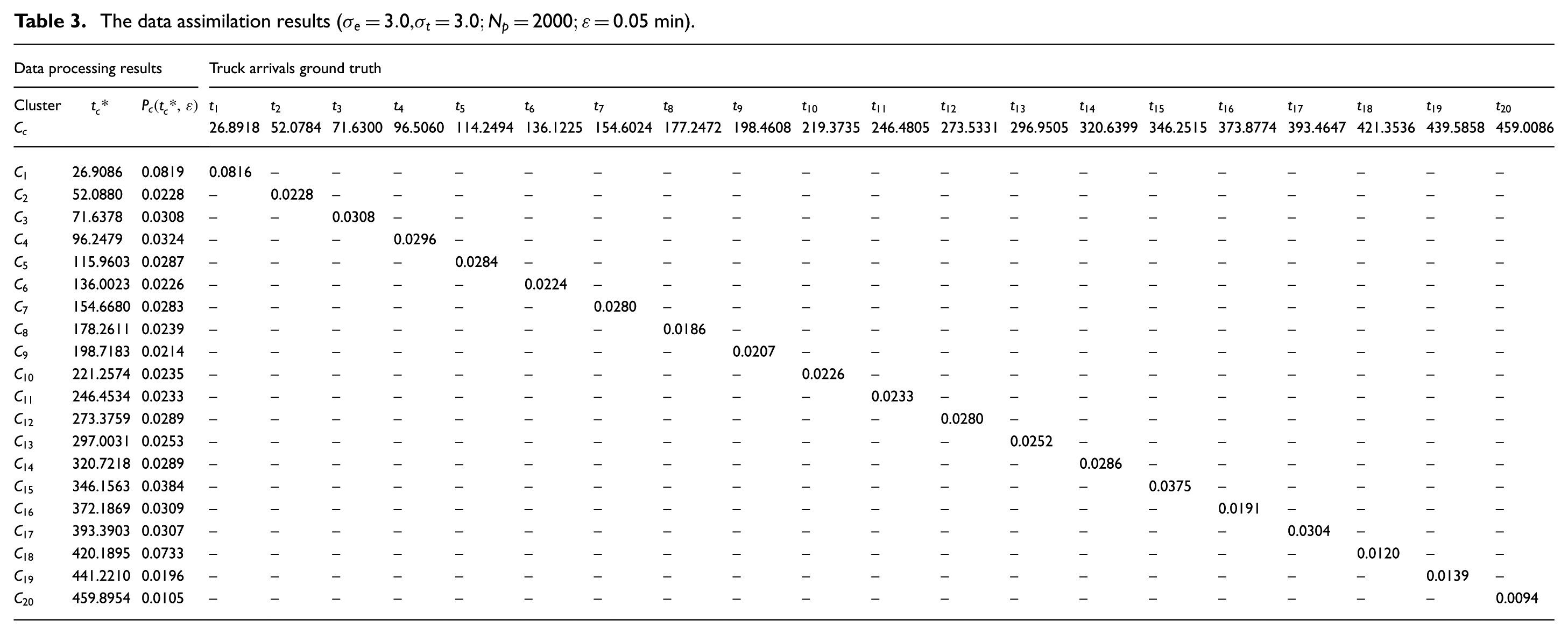
The raw estimation results shown in Figure 10(b) are clustered using the k-means clustering algorithm,
29
and the results are shown in Table 3. The k-means clustering algorithm outputs 20 clusters, that is,
The data assimilation results (
We compute the match criterion (see Equation (29)) for each truck arrival in A, and the results are depicted in Figure 14. With threshold value
success rate
waste rate
average distance
average percentage
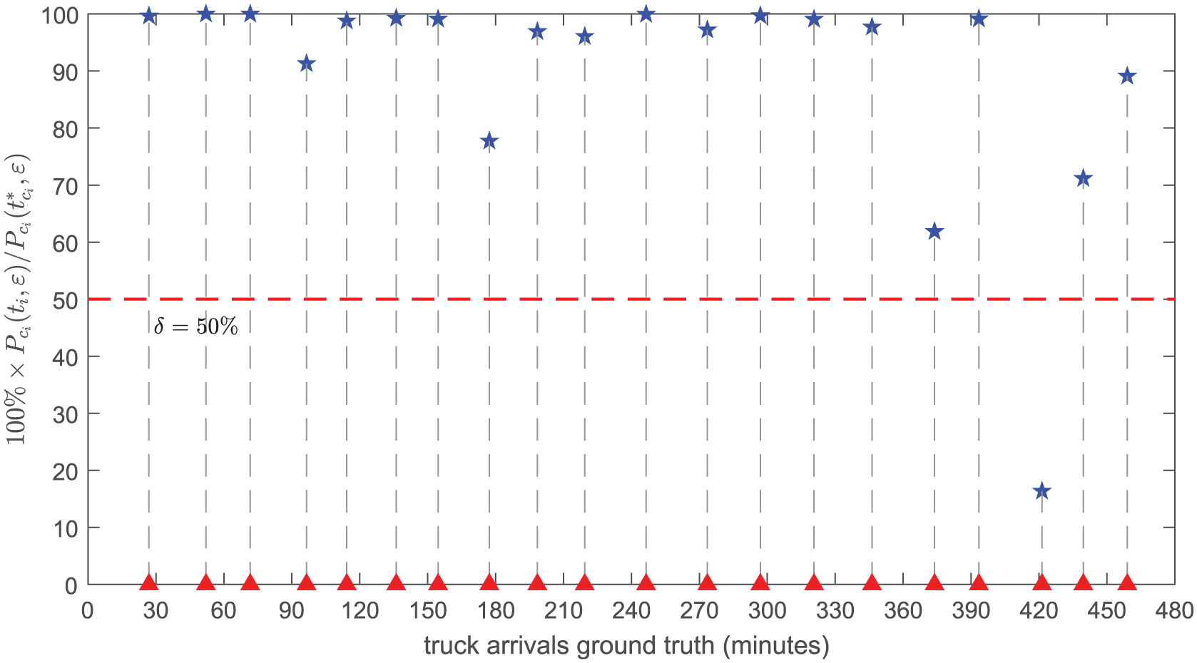
The match criterion
In the current operation of the gold mine system, the elevator only comes down when it receives a request from the miner, and therefore it will always arrive at the bottom of the vertical shaft at least 1.8 min (the difference between the time of the truck traveling full of ore and the time of the elevator going down empty) later than the trucks do. In other words, the truck will always wait at least 1.8 min until it can be served. However, using data assimilation, we can estimate 95% of all truck arrivals with an average error of 0.53 min (which is much smaller than 1.8 min). If these estimation results can be combined in the operation of the gold mine system (especially in the operation of the elevator), the overall performance of the gold mine system should be improved.
5.3.2 The effect of the interpolation operation
In this section, we explore the influence of interpolation on the estimation results. To this end, we run the data assimilation experiment 10 times with different random seeds, and draw box plots of the four error measures (i.e., SR in Equation (30), WR in Equation (31),
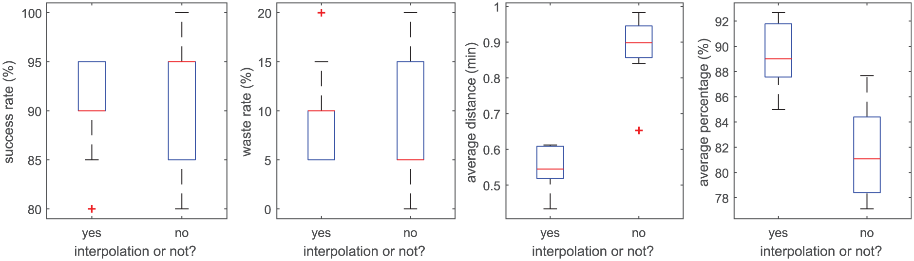
The influence of interpolation on the data assimilation results (noisy dataset (
5.4 Sensitivity analysis
In this section, we explore the influence of several key factors on the data assimilation results based on the simple gold mine case. These factors include data quality, modeling errors, and the number of particles used. For each set of parameters, we run the experiment 10 times with different random seeds.
We should note that many factors can influence the quality of the data assimilation results. Besides the factors mentioned above, other factors may include the sensor deployment information, such as the number of sensors and data collection frequency. In this simple gold mine case, we do not consider these extra factors. For a more comprehensive analysis of the particle filter-based data assimilation methods, please refer to Gu and Hu. 30
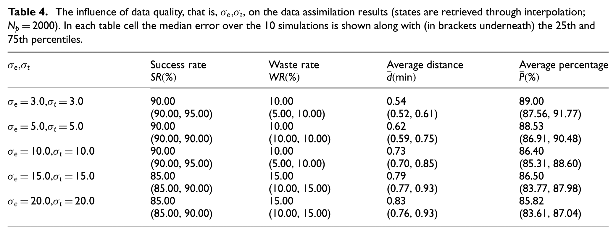
5.4.1 Effect of the data quality
In the gold mine case, only position data of entities (Elevator and Truck) are noisy, and the quality of the noisy position data is characterized by the standard deviation of the zero mean Gaussian noise, that is,
The influence of data quality, that is,
5.4.2 Effect of the model errors
In the experiment in Section 5, the model we used to carry out data assimilation is the same as that we used to generate the ground-truth data, which implies that we have a perfect model of the reality. This is a very strong assumption. In this section, we investigate the data assimilation results in the case that the model has errors. We build an imperfect model by simply changing the distribution of the drilling time of the miner from Triangular distribution with varying modes (i.e., perfect model) to a standard Triangular distribution with lower bound 15 min, upper bound 30 min, and mode 20 min (acting as the imperfect model). For all experiments, we set
The influence of model quality on the data assimilation results (states are retrieved through interpolation;
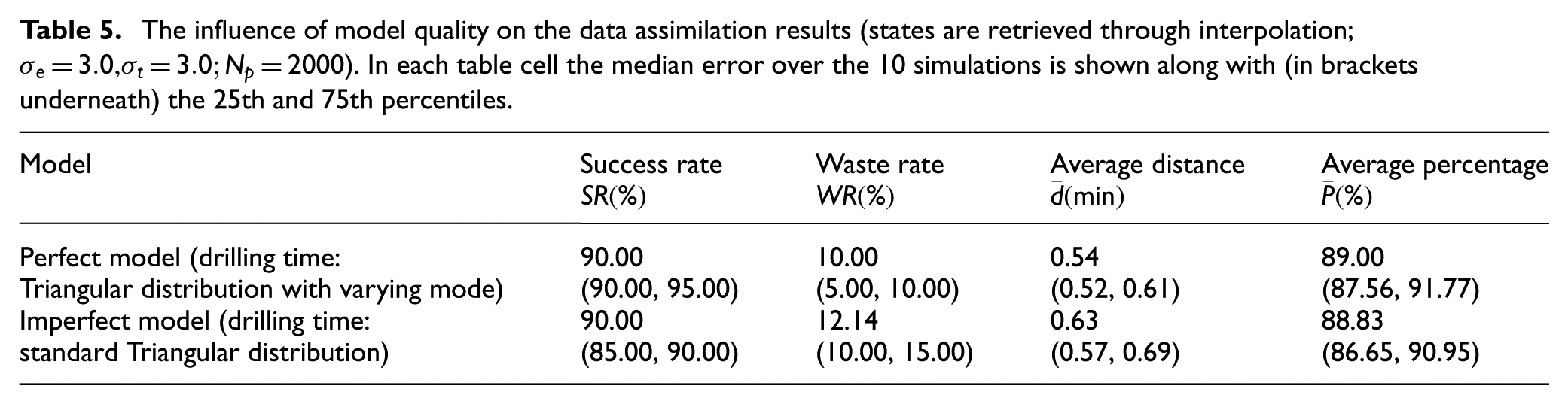
The results in Table 5 reveal that the proposed method is robust with respect to model errors, although with the case involved, we cannot claim to have tested this exhaustively. In the case that we model one component incorrectly (i.e., with a different distribution), the overall performance is not significantly different with that we use a perfect model. Clearly, the accuracy of the data assimilation results largely depends on the validity of the simulation models used. In our case, this validity is evident, since the ground-truth data is produced by a similar model.
5.4.3 Effect of the number of particles
The influence of the number of particles (
The influence of the number of particles on the data assimilation results (states are retrieved through interpolation;
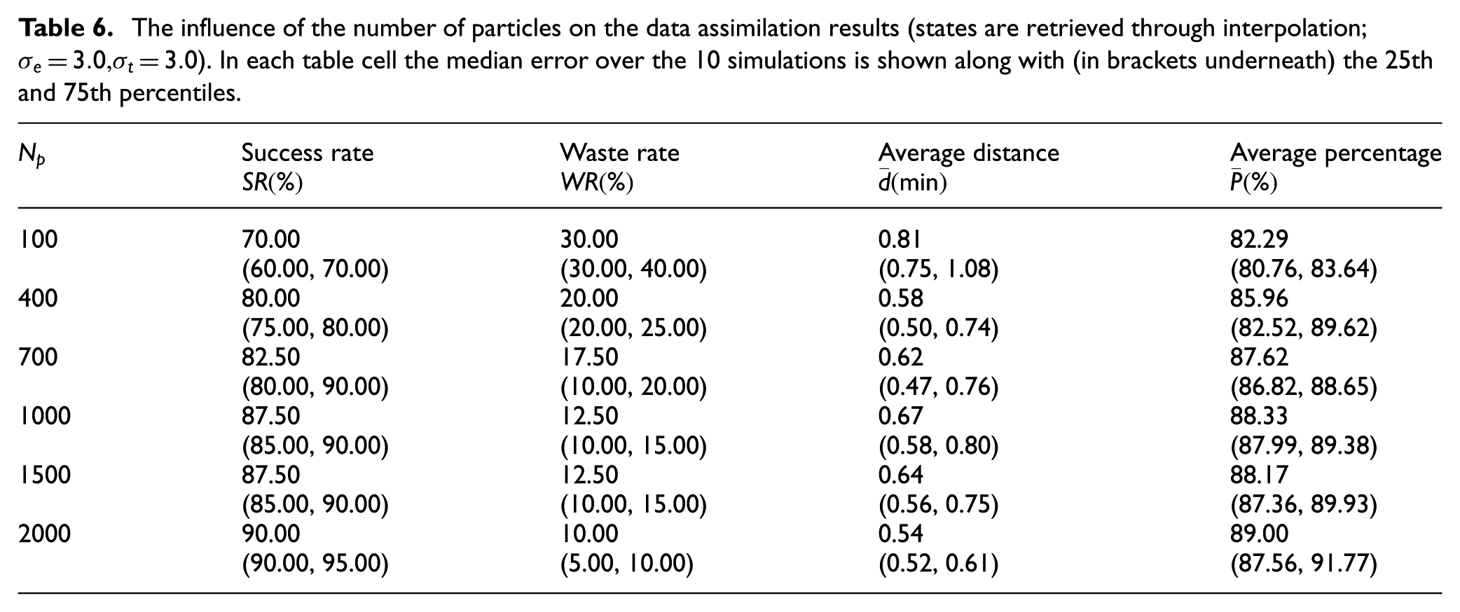
Figure 16 depicts the error measures relative to those at
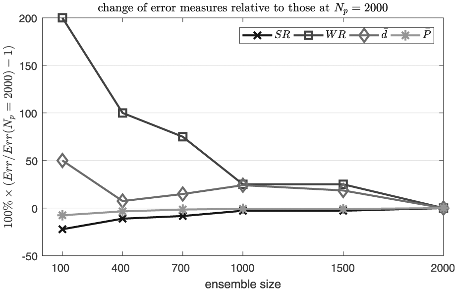
The influence of
6 Conclusions
In this paper, we presented a particle filter-based data assimilation framework for discrete event simulations (of closed systems), in which we assume that the measurements fed at time step
To illustrate the working of the proposed data assimilation framework, a case was studied in a gold mine system, in which noisy data (partial event sequences, entity positions with Gaussian errors) was assimilated into a discrete event gold mine simulation model to estimate truck arrival times at the bottom of the vertical shaft. The experiment results show that the proposed data assimilation framework is able to provide accurate estimation results in discrete event simulations. Assimilating (with interpolation) the noisy dataset with Gaussian error
Sensitivity analysis reveals that the proposed data assimilation framework is robust to error assumptions. In the gold mine case, even with a 20-m standard deviation on entity positions, the performance does not degenerate too much. Specifically, the performance indicators of estimating the truck arrivals are 85.00% (success rate), 15.00% (waste rate), 0.83 min (average distance), and 85.82% (average percentage) (see Section 5.4.1). Similarly, the framework is robust to model errors (i.e., differences between the model generating the ground-truth data and the model used in the case study), although we cannot claim to have tested this exhaustively. The result shows that using a model with errors does not significantly affect the estimation results (see Section 5.4.2). This result does, however, emphasize an important underlying point. Clearly, unless we have actual evidence (data), the accuracy of the estimation results depends on the validity of the simulation models used in the framework for the specific case at hand. In our case, this validity is evident, since the ground-truth data is produced by a similar model. In real life, when the predictions given by the simulation model diverge too much from the real behavior of the system, it stands to reason that the estimation results will be farther away from the ground truth.
The results of sensitivity analysis also imply several possible future research directions in order to improve the quality of the estimation results, such as developing simulation models that can make more valid predictions of the real system behavior, developing more advanced sensor technologies that can provide more accurate measurement data of the real systems, and developing a parallel and distributed version of the proposed data assimilation framework in order to deal with more complex scenarios.
Footnotes
Funding
This research was supported by the China Scholarship Council (Grant no. 201306110027) and the National Natural Science Foundations of China (Grant no. 61374185 and 61403402).