AUV SLAM method based on SO-CFAR and ADT feature extraction

Abstract

Due to the exceptional detection capabilities, the forward-looking sonar could be adopted in simultaneous localization and mapping (SLAM) for autonomous underwater vehicle (AUVs). This paper primarily investigates the application of the factor graph optimization SLAM algorithm based on feature maps in AUV. It achieves this by combining the smallest of constant false alarm rate (SO-CFAR) and adaptive threshold (ADT) to filter noise from the forward-looking sonar and extract feature point clouds. Furthermore, a weighted iterative closest point (WICP) algorithm is employed for feature point registration, which is extracted from the sonar image. The experimental result based on field data demonstrates that the proposed method, with an 8.52% improvement in root mean square error (RMSE) compared with dead reckoning (DR).

Introduction

Autonomous underwater vehicles (AUVs) have become crucial platforms in various fields such as seabed exploration, oceanographic mapping, and underwater emergency rescue. Achieving autonomous movement of the AUV requires addressing issues related to localization, mapping, and navigation.

AUVs require high accuracy, long endurance, and wide coverage for underwater navigation and positioning, for which simultaneous localization and mapping (SLAM) provides a key solution. SLAM allows AUVs to capture environmental features in unknown environments using a variety of sensors on board, and gradually build maps. Concurrently, the constructed map provides information feedback, allowing the AUV to adjust and optimize its localization status in real-time. ¹

In the field of underwater SLAM, cameras have been extensively utilized as sensors, showcasing impressive navigation and positioning capabilities across a multitude of environments. However, their underwater deployment is fraught with considerable challenges, predominantly attributed to the limited visibility arising from suboptimal lighting and turbid water conditions, in addition to the deleterious impact of an intricate and fluctuating underwater milieu on image clarity. These impediments substantially impede the fidelity and dependability of cameras in underwater SLAM operations.

To address these challenges, the forward-looking sonar emerges as a crucial sensor for underwater SLAM, playing a key role in precisely positioning and mapping underwater environments. It utilizes sound waves to evaluate the underwater environment, providing reliable navigation data through echo intensity analysis. This detection method offers a significant advantage, particularly in challenging conditions such as low light and visual obstructions. Integrating forward-looking sonar with existing SLAM techniques is expected to enhance the precision and robustness of underwater navigation.

Methods for SLAM map construction

This article utilizes multi-beam forward-looking sonar as an environmental sensor within the navigation system to construct an environment map. Currently, there are three current mainstream ways of describing maps of built environments: topology map based on extended space, grid map based on probability, and feature map based on feature. ²

The topological map nodes the objects in the environment, which is an abstract map description. How to node the target is a major difficulty in topology composition. The sonar data used in this paper has a low signal-to-noise ratio, which makes it more difficult to node and map.

The grid map can help the AUV in exploration, navigation, and obstacle avoidance during mission execution. However, the accuracy of a grid map is inversely proportional to the size of the grid cell, so it is difficult to balance the accuracy of the map with the complexity of storage and computation. In addition, the rasterization of the environment and objects makes it difficult for the raster map to accurately describe the outline of objects, and then achieve very accurate positioning and mapping. ²

The feature map constructs geometric representations from point and line features detected by sensors. Its advantage is evident in reduced data storage requirements and computational load and is coupled with a more intuitive depiction of environmental features. ² The accurate construction of a feature map depends on the accuracy of environmental sensors, feature extraction, and effective feature association algorithms. ³

Combining the three mapping methods mentioned above, this paper adopts a feature map to implement the AUV underwater SLAM algorithm.

AUV SLAM algorithm

SLAM algorithms can be classified into two categories. One is graph optimization, a representative form of nonlinear optimization. The other is based on Bayesian probability models, such as EKF-SLAM (Extended Kalman Filter SLAM) and Fast-SLAM (particle filter-based). These methods decompose SLAM into localization and mapping tasks. Filtering SLAM methods achieve good results and high mapping accuracy in small-scale, simple scenarios. However, in large, complex environments with many feature points, SLAM algorithms face challenges. Filtering SLAM methods rely on the Markov assumption, assuming the system state depends only on the previous moment. Graph-based SLAM methods do not rely on the Markov assumption. They record all historical states, continuously refining state estimates using subsequent observations. When loop closures are detected, they can eliminate errors in the entire trajectory. Graph-based methods extract soft constraints from SLAM control inputs and observation data, representing them using sparse graphs. The computational cost of generating the graph is low. By decomposing graph constraints into global consistency estimates, graph-based methods yield AUV pose trajectories and environmental maps.

In actual SLAM scenarios, there are situations where an AUV revisits past locations. This assumption restricts the applicability of filtering methods, leading to accumulated errors in algorithmic state estimation. Graph optimization methods are more suitable for addressing SLAM problems in large-scale scenarios compared to filtering methods, providing better accuracy in state estimation and mapping.

The rest of this paper is organized as follows. Section 2 provides a detailed description of the AUV SLAM method based on factor graph optimization. Section 3 elaborates on the proposed improved AUV SLAM algorithm. Section 4 presents the experimental results and data analysis. Finally, the paper concludes by summarizing the main findings and contributions of this research and outlining future research directions.

AUV SLAM based on factor graph optimization

AUV SLAM experimental platform

The XH-R300 AUV, which independently developed by Harbin Engineering University, is shown in Figure 1. It is designed for underwater search and rescue missions, which could be adopted for our algorithm evaluation. Equipped with a multi-beam forward-looking sonar as its primary environmental sensor, the XH-R300 integrates data from inertial measurement units (IMU) and Doppler velocity loggers (DVL) to enhance the accuracy of the SLAM algorithm. The vehicle uses GPS as ground truth for positioning, which allows for the calculation of localization error within the SLAM algorithm and facilitates subsequent performance analysis and comparison. Figure 2 illustrates the deployment of the main sensors within the SLAM system on the “XH-R300”. The three-dimensional exterior of the “XH-R300” is depicted in Figure 1, followed by an introduction to the sensors carried by the AUV.

1. Inertial Measurement Unit (IMU)

Figure 1.

Exterior view of an AUV, depicting its three-view projection.

Figure 2.

“XH-R300” AUV sensor deployment Diagram2.

The IMU is a critical sensor for the underwater navigation of AUVs. Its main components include accelerometers and gyroscopes, which measure the three-axis acceleration and angular velocity of the AUV. Based on this information, the IMU can calculate the heading and attitude of the AUV in real-time using motion differential equations.

2. Doppler Velocity Log (DVL)

The DVL is a sensor that utilizes the Doppler effect of emitted sound waves to measure velocity. By analyzing the Doppler frequency shift, the velocity of the AUV relative to a sound reflection source (such as the seafloor) can be calculated in the coordinate system of vehicle.

• 3. Depth Meter

The Depth Meter is a type of sensor used to measure the depth of underwater bodies of water. Its principle of operation involves measuring water pressure and then calculating the distance from the surface to the vehicle based on water density and gravitational acceleration. Depth Meter measurements do not accumulate errors, ensuring accurate data. Once calibrated, they can be readily applied to navigation systems without requiring excessive processing.

• 4. Global Positioning System (GPS)

The GPS is a satellite navigation system capable of providing highly accurate positioning information around the clock. GPS offers location data independent of past values and does not suffer from accumulated errors.

• 5. Forward-Looking Sonar (FLS)

The FLS emits sound waves forward in both horizontal and vertical directions, receiving echo signals reflected by the environment and targets. Based on these echo signals, distance and bearing information between the target and the vehicle can be obtained. Additionally, echo intensity is stored as grayscale values, forming underwater acoustic images along the beam direction.^3,4

Factor graph framework for AUV SLAM

The AUV SLAM graph optimization method models the SLAM problem as an optimization problem, primarily consisting of two parts: the front-end and the back-end. The front-end is responsible for graph construction, utilizing image frames obtained by sensors at different time steps. The front-end introduces a probabilistic graph model via factor graphs to solve the optimization problem, typically employing algorithms such as ICP for feature point registration, determining pose transformations between adjacent domains, and completing fusion between image frames to reconstruct the map. The back-end conducts graph optimization calculations, typically implemented based on the Least Squares Method.

The AUV SLAM algorithm constructs a pose graph in the form of a factor graph. This factor graph excludes landmark nodes and observation factors, consisting solely of AUV pose nodes and sequential scan matching (SSM) factors connected to these nodes. Optimization is exclusively focused on the AUV pose trajectory. The SSM factors represent constraints between AUV poses, incorporating estimates derived from Dead Reckoning (DR) using IMU and DVL, or sonar image feature matching results. The algorithm evaluates feature matching results and selects, according to a specific strategy, whether to use dead reckoning or pose estimates obtained from feature matching. Consequently, both DR and sonar constraint factors are integrated into the graph. Prior estimation serves as the starting point for Bayesian inference, updating parameter estimates by combining observed data. The structure of the factor graph is depicted in Figure 3, where p represents prior estimation, x denotes the AUV poses, u indicates the DR factor, and s represents the sonar constraint factors.

Figure 3.

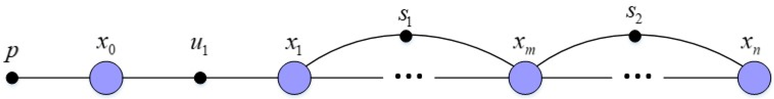
Structure of the AUV SLAM factor graph.

Establishment of DR factors

Establishing the Dead Reckoning measurement model:

$$z_i^{dr}=f(x_i,x_{i+1})+{\omega }_i$$

(1)

Where, $f(x_i,x_{i+1})$ denotes the navigation estimation generation model between two consecutive poses, $x_i$ and $x_{i+1}$ , of an AUV. ${\omega }_i$ is the Gaussian noise, where its covariance is directly proportional to the time interval between the two poses.

DR Generation Model:

$$f(x_i,x_{i+1})=\left[\begin{array}{c}dx\\ dy\\ d_{\psi }\end{array}\right]=\left[\begin{array}{c}{u}_i\cos ({\psi }_i)dt-v_i\sin ({\psi }_i)dt\\ u_i\sin ({\psi }_i)dt-v_i\cos ({\psi }_i)dt\\ {\psi }_I-{\psi }_i\end{array}\right]$$

(2)

Where, the represents the northward and eastward displacement changes, as well as the variation in course angle, of the AUV from its previous position and posture $x_i$ to the current position and posture $x_{i+1}$ . $dt$ refers to the time interval between these two consecutive positions and postures. In the local coordinate system at position and posture $x_i$ from the previous moment, $u_i$ and $v_i$ represent the forward velocity and starboard velocity measured by the DVL, respectively. ${\psi }_i$ denotes the heading angle of the AUV at the previous moment, while ${\psi }_i$ represents the heading angle measured by the IMU at the current moment.

By integrating the DR measurement model with navigation sensor data, one can derive the pose transformation equations between two consecutive pose nodes, which facilitates the computation of the DR measurement factor.

Establishment of sonar constraint factors

The key to calculating sonar constraint factors is the registration of sonar image frames, which involves estimating the pose transformations between consecutive sonar images. This process specifically involves steps like feature extraction and feature matching from sonar images. Currently, underwater sonar image matching techniques can be primarily categorized into three methods: feature-based methods, region-based methods, and methods that rely on matching based on the entire image content.^5,6

Feature-based methods focus on extracting distinguishable point or line features that can be observed repeatedly in sonar images. By matching these features, the corresponding algorithms establish correspondence relationships between sets of features in the two images, thereby estimating the relative pose change between the image frames.

Johannsson et al. employed a region-based approach to realize the feature extraction and matching of sonar images. ⁷ They identified and extracted local region features from sonar images that exhibit significant changes in acoustic intensity, such as object-shadow transition boundaries. Hurtos used a similar technique to extract two types of regional features in sonar images ⁸ : one type consists of pixels with the highest acoustic intensity typically associated with positions on the observed target objects; the other comprises pixels with negative vertical gradient characteristics, corresponding to object-shadow boundaries within the images ⁹ :

Methods that utilize the entire image content during the image registration process incorporate more information to minimize registration errors. However, these methods are generally not ideal for handling highly complex pose estimation problems and require substantial overlap between the images being registered.

Due to the inherent noise and low resolution of sonar data, pixel-level features extracted using feature descriptors from sonar images often have low repeatability and stability, increasing the risk of false matches and inaccurate pose constraints. Moreover, accurate feature extraction and matching become more challenging when dealing with loop-closure situations or time-separated sonar images taken at considerable intervals. Therefore, this paper proposes extracting point cloud features from sonar images and using solely geometric information from the point clouds to match sonar image frames via the ICP algorithm, thus estimating the necessary pose constraints.

ICP algorithm workflow

The ICP algorithm is currently the most widely applied method for precise registration of point clouds. Its principle is as follows: from the source and target point clouds to be matched, the algorithm searches for the nearest points, establishes correspondences among these points, and constructs an error function using the mean square error between matched points. Iteratively, the algorithm computes rotational and translational transformations that minimize this error. Simultaneously, based on the nearest-point selection principle, the matching relations are updated throughout the process. Ultimately, the algorithm continues iterating until the matching error is below a threshold, achieving the optimal transformation between the source and target point clouds.

The following presents the specific implementation process of the ICP algorithm: Given the target point cloud X and the source point cloud P as follows:

$$\begin{array}{c}X=\{x_1,x_2,\cdots ,x_m\}\\ P=\{p_1,p_2,\cdots ,p_n\}\end{array}$$

(3)

In the context, $x_i$ and $p_i$ represent individual points within point sets. In practical scenarios, the matching relationships between the two sets of point clouds are unknown, and the number of points in each cloud may vary. The goal is to solve for the relative pose between the point clouds, denoted by R and t, where R signifies a rotation matrix representing the orientation and t represents a translation vector indicating the positional difference. The algorithm steps are as follows:

1. Remove the centroids of the source and target point clouds

   Calculate the centroid of two sets of point clouds: ${\mu }_x={\displaystyle \frac{1}{n}\sum _{i=1}^n{x}_i,{\mu }_p={\displaystyle \frac{1}{n}\sum _{i=1}^n{p}_i}}$

   After removing the centroids, the point cloud coordinates become: $X^{\mathrm{\prime }}=\{x_i-{\mu }_x\}=\{x_i^{\mathrm{\prime }}\},P^{\mathrm{\prime }}=\{p_i-{\mu }_p\}=\{p_i^{\mathrm{\prime }}\}$

2. Define $\mathit{W}=\sum _{i=1}^n{x}_i^{\mathrm{\prime }}{(p^{\mathrm{\prime }})}^T$

3. Compute the rotation matrix R.

   Perform singular value decomposition (SVD) on $\mathbf{W}$ to obtain $\mathbf{W}=\mathbf{U}\mathbf{\Sigma }{\mathbf{V}}^{\mathbf{T}}$ , where $\mathbf{U}$ and $\mathbf{V}$ are both orthogonal matrices, and $\mathbf{\Sigma }$ is a diagonal matrix. When $\mathbf{W}$ has full rank, there exists a unique solution:

   $$\mathbf{R}=\mathbf{U}{\mathbf{V}}^{\mathbf{T}}$$

   (4)

4. Compute the translation $\mathbf{t}={\mu }_x-\mathbf{R}{\mu }_p$

Thus far, the point cloud matching problem under known correspondences has been solved. However, in practical scenarios, the correspondence between points in the two sets of point clouds is unknown, and the number of points may differ. Consequently, the ICP algorithm employs an iterative solution method to compute the pose transformation between point clouds. The iterative computation steps are as follows:

Finding the nearest points to establish point correspondences

Computing the pose transformation between point clouds

Determining whether the termination criteria for the iterative process are satisfied

Improved graph optimization SLAM method based on SO-CFAR and ADT

In underwater environments, traditional SLAM algorithms often fail to fully utilize the information in sonar images. This leads to the creation of sparse feature point clouds that do not adequately represent the surroundings, which in turn results in low point cloud matching accuracy and imprecise pose transformation estimations between sonar frames.^10,11 To address these issues, we have developed an enhanced SLAM method that integrates SO-CFAR and ADT techniques.

This approach focuses on the accurate and comprehensive extraction of environmental features from the entire sonar image domain. It combines CFAR techniques with ADT segmentation to derive feature point clouds from sonar imagery. Additionally, it employs a weighted ICP method for sonar feature point cloud matching. The proposed method incorporates IMU, DVL, and forward-looking sonar data into a factor graph optimization algorithm, utilizing the iSAM2 incremental smoothing and mapping framework within the GTSAM factor graph optimization library.^12–14 The algorithm is implemented using the robot operating system (ROS), which synchronizes data from various sensors and constructs the necessary functional nodes for the SLAM process, including front-facing sonar image feature extraction, feature matching, DR, and backend optimization. The detailed flowchart of the algorithm is shown in Figure 4. The schematic diagram of the algorithm nodes and their connections is shown in Figure 5.

Figure 4.

shows the framework of the improved AUV SLAM algorithm.

Figure 5.

The connectivity diagram of SLAM algorithm nodes and connection methods.

Sonar feature point cloud extraction based on SO-CFAR

Principles of CFAR algorithm

CFAR is used in systems to detect targets amid noise and clutter. It establishes a dynamic detection threshold based on local noise and clutter levels. In traditional SO-CFAR, the grayscale values of characteristic points are extracted. This study employs a one-dimensional SO-CFAR method to process echo signals in each beam, extracting feature point clouds from sonar images. SO-CFAR combines sparse representation with CFAR for accurate detection and estimation in signal processing, even with many zero values. Sonar signal target detection follows a binary hypothesis testing model framework.

$$\{\begin{array}{c}{H}_1:\lambda >\eta \\ H_0:\lambda \le \eta \end{array}$$

(5)

In this context, $\lambda$ represents the detection statistic formed by the sonar echo data, and $\eta$ is the detection threshold set according to the desired false alarm probability. $H_0$ and $H_1$ respectively represent the hypotheses “target absent” and “target present”.

The number of protection units and reference units should be configured according to the parameters such as the resolution of the sonar sensor and the actual observation data. It is assumed that the number of reference units is $2n$ . In this study, the radial distance resolution of the forward-looking sonar image is 0.28–0.38 m. For the CFAR algorithm applied, 10 guard cells and 46 reference cells are set on either side of the detection cell.

Set the target detection threshold as $T=\tau \times Z$ , where Z is the estimated power of background clutter, and $\tau$ is the threshold factor. If the sampled signal $Y>T$ in the detection unit meets the condition, a target is deemed present; otherwise, it is considered not present. Figure 6 is the schematic diagram of the CFAR detection used in the forward-looking sonar in this paper.

Figure 6.

illustrates the principle diagram of forward-looking sonar CFAR detection.

After square-law detection, clutter and noise follow an exponential distribution. The probability density function PDF for the sampled signals in the reference cells is given by:

$$T=\tau \times Zf(x)={\displaystyle \frac{1}{2\mu }{e}^{-\frac{x}{2\mu }},x\ge 0}$$

(6)

In this expression, $\mu$ represents the noise power, and x denotes the sampled signal within the reference cells.

$P[Y>\tau Z|H_0]$ denotes the probability of mistakenly identifying a target when there is none, which is the false alarm probability, and its expression is given as:

$$\begin{gathered} P_{fa}=E_Z\left\{P\left[Y>\tau Z|H_0\right]\right\} \\ =E_Z\left\{{\int }_{\tau Z}^{\mathrm{\infty }}f(y)dy\right\}=E_Z\left\{{\int }_{\tau Z}^{\mathrm{\infty }}(1/2\mu )\text{e}(-y/2\mu )dy\right\} \\ =E_Z\{\text{e}(-\tau Z/2\mu )\} \end{gathered}$$

(7)

In this equation, Y represents the set of samples from the detection unit, while $y$ refers to an individual sample signal.

The relationship between the false alarm probability $P_{fa}$ and the threshold factor $\tau$ can be further derived:

$$P_{fa}=(1+\tau {)}^{-2n}\iff \tau =(P_{fa}{)}^{-1/2n}-1$$

(8)

Assuming the echo intensity in the reference units is represented by the sequence $\{I_1,I_2,\cdots ,I_n,I_{n+1},I_{n+2},\cdots ,I_{2n}\}$ , which corresponds to the grayscale values of pixel elements in the sonar image, and the average echo intensity for the leading and trailing reference units is denoted as:

$$\{\begin{array}{c}{T}_1={\displaystyle \frac{1}{n}\sum _{i=1}^n{I}_i}\\ T_2={\displaystyle \frac{1}{n}\sum _{i=n+1}^{2n}{I}_i}\end{array}$$

(9)

Then, the SOCA-CFAR detection threshold for the detection unit is:

$$T=\tau \min (T_1,T_2)$$

(10)

Here, $\tau$ represents the threshold factor. Given a specified false alarm probability $P_{fa}$ , the threshold factor t can be calculated using the following formula:

$$P_{\mathrm{fa}}={\left(2+{\displaystyle \frac{\tau }{n}}\right)}^{-n}\sum _{i=0}^{n-1}\left(\begin{array}{c}n-1+i\\ i\end{array}\right){\left(2+{\displaystyle \frac{\tau }{n}}\right)}^{-n}$$

(11)

Calculating the threshold factor enables one to determine the detection threshold, which is crucial for assessing the presence of a target within the detection unit. This process is vital for sonar image CFAR detection, as it involves identifying the pixels within the image that represent the echo signals from environmental targets.

Polar coordinate feature points can be transformed into 2D point cloud P in the Cartesian coordinate system using the following formula: $\{p=(x_i,y_i)|0\le i\le n\}$

$$\{\begin{array}{c}{x}_i=r_i\cos ({\theta }_i)\\ y_i=r_i\sin ({\theta }_i)\end{array}$$

(12)

Figure 7 shows the effectiveness of the SO-CFAR method for extracting feature points, and presents the resulting feature point clouds in both polar and Cartesian coordinate systems. In the figure, (a) depicts the original polar sonar image, (b) displays the feature point cloud extracted by the SO-CFAR method from this polar image, and (c) presents the same feature point cloud in a Cartesian coordinate system.

Figure 7.

Visualization of CFAR extracted feature point cloud.

The SO-CFAR method effectively extracts feature points corresponding to target objects in forward-looking sonar images, but it does not eliminate all image noise. Furthermore, irrelevant targets, such as underwater bubbles, are also detected. Therefore, it is necessary to establish a particular sound intensity threshold to refine the extracted feature points.

ADT for point cloud filtering and extraction

ADT is utilized to segment target and background areas within images. In contrast to global thresholding methods, which apply a fixed threshold across the entire image, ADT is tailored for processing images with uneven grayscale or noise, such as sonar images.^15–17 This method adaptively calculates local thresholds based on the brightness levels across different image regions, enabling more accurate segmentation of target areas.

In the previous SO-CFAR step, grayscale values of characteristic points are extracted to obtain the final characteristic point cloud using a combined adaptive and fixed thresholding approach for further filtering. ADT finely segments features distinguishable from the background environment in sonar images, employing a lower fixed threshold to prevent excessively low local thresholds, thereby avoiding the introduction of noise and artifacts that could negatively impact navigation calculations. ADT determines local thresholds by computing a two-dimensional Gaussian weighted average of neighboring pixel grayscale values. This Gaussian weighted average considers the grayscale distribution around each pixel, effectively adapting to local brightness variations in the image:

$$g(x,y)={\displaystyle \frac{1}{2\pi {\sigma }^2}{e}^{-\frac{(x^2+y^2)}{2{\sigma }^2}}}$$

(13)

In the formula, $(x,y)$ represents the coordinates of a pixel point.

The grayscale value range of sonar image pixels is $[0,255]$ . For the fixed threshold, based on empirical tuning in this paper, a fixed threshold $\mathrm{Th}=15$ is chosen. Suppose $\mathrm{p}$ is a feature pixel point detected by SO-CFAR, with a grayscale value $\mathrm{g}$ . A pixel point will only be recognized as a final feature point if it satisfies the following conditions simultaneously:

$$\left\{\begin{array}{c}g>Th\\ g>ADT(p)\end{array}\right\}$$

(14)

Here: $ADT()$ is the function to calculate the ADT for a particular pixel point in the image.

The process proposed in this article for extracting feature point clouds from sonar images can be described by the following Figure 8.

Figure 8.

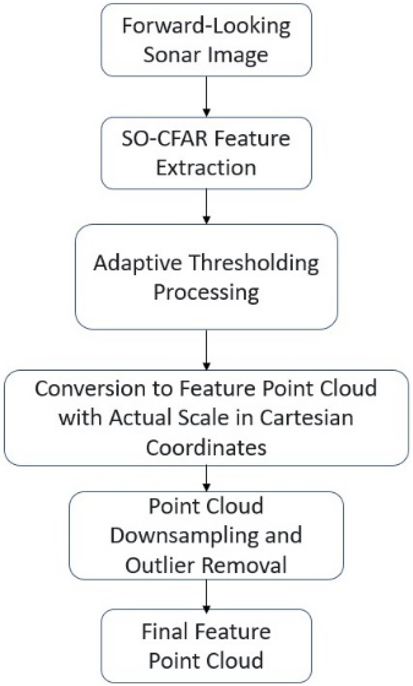
Flowchart of forward-looking sonar feature point extraction process.

The application of the feature point extraction algorithm to sonar images from various underwater environments is shown in Figure 9.

Figure 9.

Sonar image feature point extraction procedure and results.

Figure 10.

Sonar Observation Geometry Principle.

Figure 9(a) illustrates an underwater forest environment within a lake bay, while Figure 9(b) depicts a floating dock. The figure demonstrates that the proposed feature extraction method effectively processes sonar images from complex underwater environments, accurately extracts feature point clouds, and reduces image noise.

ADT parameter is influenced by threshold parameters, window size, and noise models. Threshold parameters are chosen based on statistical models of noise and signal-to-noise ratio. The size of the detection window is selected to balance sensitivity and robustness between the expected duration of the signal and fluctuations in noise. Noise models are estimated from historical data or assumed based on known environmental conditions. SO-CFAR adjusts detection thresholds based on local noise statistics while considering signal stretching.

Weighted ICP-based sonar point cloud matching

The traditional ICP algorithm heavily depends on the initial values of point cloud data and requires high consistency between two sets of point clouds. Otherwise, the solution is prone to local optima, leading to inefficient iterative calculations and reduced accuracy of the results. In the matching of sonar point clouds, since the noise in the sonar data cannot be entirely removed, and there is an inherent uncertainty in the position of sonar point clouds due to the principles of sonar observation, this paper proposes a weighted ICP algorithm using geometric analysis of sonar observations for registering point clouds that underwent SO-CFAR and ADT feature extraction.

Based on the principles of sonar observation, there is an inherent uncertainty in the position of sonar point clouds. Using a weighted ICP algorithm that employs geometric analysis of sonar observations, and using pose transformations obtained from IMU and DVL DR data, the initial matching of point clouds is performed to ensure the consistency of the data being matched.^18,19

The Weighted Iterative Closest Point (WICP) method enhances point cloud registration performance by integrating weighting mechanisms into the iterative closest point pairing process. After calculating the optimal transformation using Singular Value Decomposition (SVD), the method iteratively refines the alignment until it converges.^20–22 This approach significantly improves both the accuracy and robustness of the registration.

Based on the description in Figure 10, the sonar's observation range is $[r_{\min },r_{\max }]$ , the horizontal field of view angle spans $\left[-\frac{{\psi }_{\max }}{2},\frac{{\psi }_{\max }}{2}\right]$ , and the vertical field of view angle is $\left[-\frac{{\varphi }_{\max }}{2},\frac{{\varphi }_{\max }}{2}\right]$ . Assuming that a feature point p has an azimuth angle $\psi$ , depression angle $\varphi$ , and range r, in the sonar observation coordinate system $xyz$ .^23–25 The beam spacing is denoted as ${\psi }_{res}$ . An approximate area integral over the arc surface S, can be expressed as:

$$S=r^2{\psi }_{\max }{\varphi }_{\max }$$

(15)

The size of the arc area S is directly proportional to $r^2$ , where the larger the arc area, the higher the uncertainty of the feature point's position derived from observational data. For all points in the matched point cloud, we compute their corresponding arc area $\{S_i|i=1,2,\cdots ,n\}$ , where n represents the total number of points. The uncertainty of a point can be represented in a logarithmic form based on its area proportion:

$$k_i={\displaystyle \frac{S_i}{\sum S_i},w_i=ln{\displaystyle \frac{1}{k_i}}}$$

(16)

Here, $k_i$ indicates the proportion of the arc area occupied by the feature point within the total area, $w_i$ stands for the uncertainty of the point, which also serves as its weight. The logarithmic form is adopted to avoid significant disparities in the weights among the points in the point set.

The matching error function in the ICP algorithm is modified to:

$$E(R,t)={\displaystyle \frac{1}{n}{\sum }_{i-1}^n{w}_i||x_i-(R{p}_i+t)|{|}^2}$$

(17)

Correspondingly, the computation process for this matching error function is modified to:

$$W=\sum _{i=1}^n{w}_i{x}_i^{\mathrm{\prime }}{(p^{\mathrm{\prime }})}^T$$

(18)

The remaining computational steps remain unchanged, ultimately yielding an improved weighted ICP method based on sonar observation geometry analysis. Subsequently, the initial pose transformation obtained from DR will be incorporated to perform weighted ICP matching of the sonar point cloud data.

According to the model derived from DR calculations, we obtain the initial pose transformation $T_{dr}=[dx,dy,d\psi {]}^T$ from the previous sonar observation posture to the current one for the AUV, where $dx,dy,d\psi$ represent the displacements in the northward and eastward directions and the heading rotation angle, respectively. In the vehicle coordinate system of the AUV, the previous sonar observation is taken as the target point cloud $C_t$ , while the current observation serves as the source point cloud $C_s$ . The specific steps to calculate the pose transformation from the source point cloud to the target point cloud are as follows:

Based on the initial pose transformation $T_{dr}$ , perform an initial transformation on the source point cloud. The rotation matrix R, displacement vector t, and transformation matrix H from the previous pose to the current pose are:

$$\left\{\begin{array}{c}R=\left[\begin{array}{cc}\cos d\psi & -\sin d\psi \\ \sin d\psi & \cos d\psi \end{array}\right]\\ t={\left[\begin{array}{cc}dx& dy\end{array}\right]}^T\\ H=\left[\begin{array}{cc}R& t\\ 0& 1\end{array}\right]\end{array}\right\}$$

(19)

After the initial transformation, the source point cloud becomes:

$$C_s^{\mathrm{\prime }}=\mathbf{H}{C}_s$$

(20)

In the above expression, point cloud coordinates are converted into homogeneous coordinates for participation in the computation.

Employ the weighted ICP algorithm to iteratively compute the pose transformation (rotation matrix R and translation vector t) from the source point cloud Cs to the target point cloud Ct, and update the pose transformation accordingly:

$$\left\{\begin{array}{c}{R}_{st}=R^{\mathrm{\prime }}R\\ t_{st}=t+t^{\mathrm{\prime }}\\ H_{st}=\left[\begin{array}{cc}{R}_{st}& t_{st}\\ 0& 1\end{array}\right]\end{array}\right\}$$

(21)

Here, $R_{st}$ represents the rotation matrix describing the orientation change needed to align the source point cloud $C_s$ with the target point cloud $C_{\mathrm{t}}$ , $t_{st}$ is the translation vector signifying the positional shift required to bring $C_s$ closer to $C_{\mathrm{t}}$ , and $H_{st}$ is the combined transformation matrix that incorporates both rotation and translation, effectively capturing the complete pose transformation from $C_s$ to $C_{\mathrm{t}}$ .

Let $H=H_{st}$ repeat Step (1) using Equation 39 and Step (2) until the convergence criterion for the ICP algorithm is met, thus achieving the optimal pose transformation between the point clouds.

Experimentation and data analysis

The experimental data was collected at Danjiangkou Reservoir in Nanyang, Henan, using ‘XH-R300’ equipped with forward-looking sonar, IMU, GPS, and DVL, to validate the effectiveness of the SO-CFAR and ADT enhanced SLAM algorithm in complex underwater environments. Experiments were conducted to substantiate the performance of the improved algorithm, comparing the results with DR and GPS positioning data. Trajectory comparison charts and error comparison diagrams were drawn to illustrate the experimental outcomes.

AUV collected experimental data in the forest bay waters, as shown in Figure 11(b). These data were utilized in the SLAM algorithm, which was optimized with a factor graph and is presented in this paper. The algorithm's accuracy was assessed using the SLAM mapping and precision assessment tool EVO. The positioning trajectory of the algorithm is depicted in Figs 12 and 13.

Figure 11.

Illustration of experimental environment.

Figure 12.

Comparison of positioning trajectories.

Figure 13.

Comparative plots evaluating algorithm accuracy using the precision evaluation tool EVO, showing position trajectories in the north-east coordinate system. These plots visually depict the spatial distribution and relative errors of the trajectories, aiding in the assessment of algorithm performance under different conditions and providing quantitative insights into accuracy.

From Figure 12, it can be observed that compared to DR, the positioning trajectory of the SLAM algorithm is closer to the GPS trajectory throughout the entire process. Figure 13 compares the positioning in various coordinate directions; the positioning by the SLAM algorithm is closer to the true value, which is the GPS location, in all directions, further verifying the accuracy of the algorithm's positioning and its ability to suppress positioning errors. In the depth direction, since all positioning methods directly use the values from the Depth Meter gauge, they perform identically.

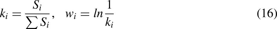
The Absolute Pose Error (APE) and Root Mean Square Error (RMSE) are essential metrics for evaluating the performance of the SLAM algorithm and DR conducted by EVO. In SLAM, using APE and RMSE to evaluate the trajectory serves specific purposes: APE is suited for assessing precision at instantaneous or specific time points, especially crucial for ensuring high-precision localization. RMSE, on the other hand, is apt for evaluating accumulated errors over extended durations or large-scale movements, aiding in identifying potential drift or cumulative error issues within the system.^26–28 APE quantifies the translational error within the trajectory, calculated using the formula:

$$APE={\displaystyle \frac{1}{N}{\mathrm{\Sigma }}_{i=1}^N||t_i-\widehat{t_i}||}$$

(22)

where $t_i$ and $\widehat{t_i}$ are the ground truth and estimated translations at time step i, respectively, and N is the number of poses.

RMSE provides an overall measure of the error distribution and is defined as:

$$RMSE=\sqrt{{\displaystyle \frac{1}{N}{\mathrm{\Sigma }}_{i=1}^N||t_i-\widehat{t_i}|{|}^2}}$$

(23)

In Figure 14(a) and 15(a), we present the RMSE, median, mean, and standard deviation of the APE, highlighting the statistical distribution of the translational errors. Additionally, Table 1 provides a comparative summary of these statistical measures for the APE calculation outcomes.

Figure 14.

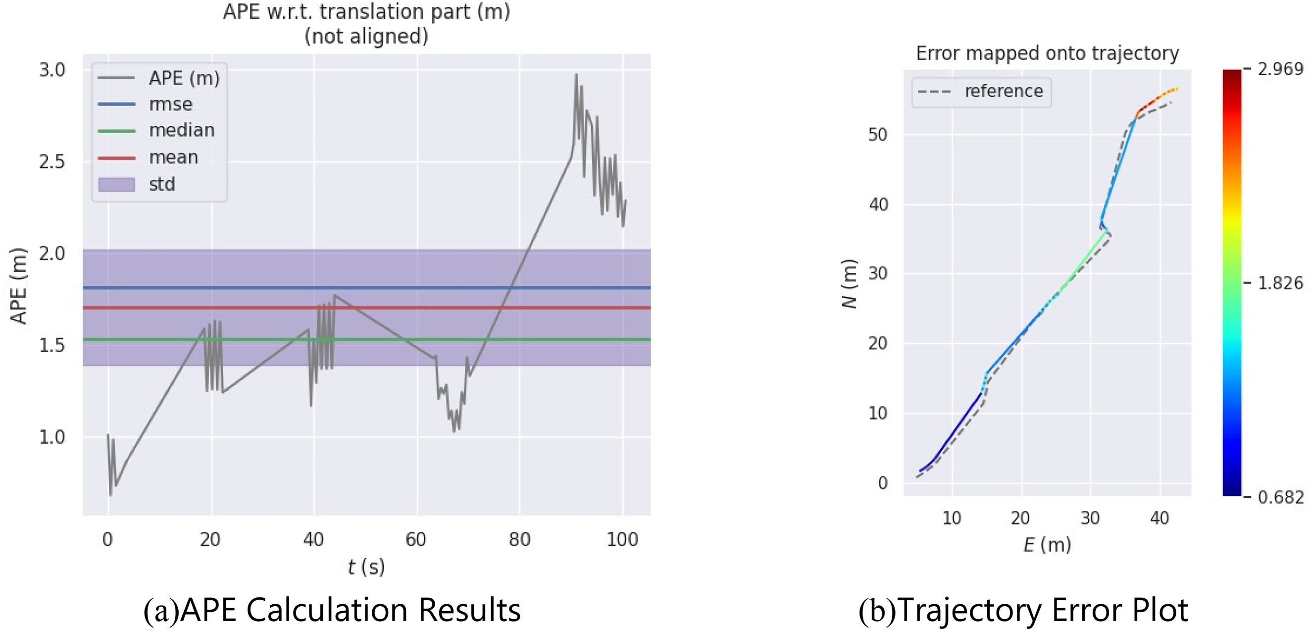
Using EVO for absolute pose error evaluation in SLAM trajectories, and examines RMSE, median, mean, and standard deviation of APE.

Figure 15.

Evaluates APE in dead reckoning trajectories using EVO, analyzing its RMSE, median error, mean error, and standard deviation.

Table 1.

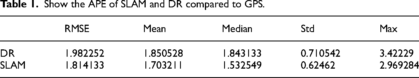
Show the APE of SLAM and DR compared to GPS.

	RMSE	Mean	Median	Std	Max
DR	1.982252	1.850528	1.843133	0.710542	3.42229
SLAM	1.814133	1.703211	1.532549	0.62462	2.969284

APE and RMSE, as emerging SLAM evaluation metrics, offer significant advantages over traditional benchmarks like ATE and RPE. They not only provide detailed analysis of pose accuracy at specific time points (APE), but also comprehensively assess cumulative errors and stability over long-term operations (RMSE).^29,30 This enhances insights into and operational capabilities for optimizing SLAM system performance in complex environments.

Figures 14 and 15, along with Table 1, reveal that the trajectory error associated with the SLAM algorithm is generally lower than that of DR. Additionally, the APE statistical indicators for the SLAM algorithm are also lesser. Based on the calculations, the actual traveled distance during the experiment was 88.966 m. The positioning accuracy, when assessed using RMSE, was 2.23% for DR and 2.04% for the SLAM algorithm. This indicates that the SLAM algorithm enhanced the positioning accuracy by approximately 8.52% in comparison to DR.

The feature map constructed using the SLAM algorithm is depicted in Figure 16. In this figure, the green line represents the SLAM trajectory, while the colored points represent the feature points. The feature map generated by the SLAM algorithm presented in this study effectively captures the contours of the submerged underwater terrain. This indicates that the SLAM algorithm can be successfully applied to navigate complex underwater settings.

Figure 16.

Diagram of the feature map constructed by the SLAM algorithm.

The SLAM method, incorporating SO-CFAR and ADT for sonar image filtering, achieves an 8.52% performance improvement compared to traditional methods. This advancement is attributed to advanced algorithms, sensor fusion, and parameter optimization, enhancing pose accuracy and long-term stability of the system. The introduction of metrics like APE and RMSE contributes to a comprehensive evaluation. The implications include enhanced application robustness and operational efficiency in fields such as autonomous driving and robotics.

Conclusion

This paper presents an improved Factor Graph Optimization SLAM algorithm, based on SO-CFAR and ADT. First, the adopted Factor Graph SLAM framework is introduced, along with the methods for constructing factors within the graph model. Next, the process and methodology for extracting feature point clouds from sonar images using SO-CFAR and ADT segmentation are described. Following this, the paper proposes an improvement upon the traditional ICP algorithm, which implements a Weighted ICP method for registering sonar feature point clouds. Subsequently, the validity of the proposed algorithm is verified through experiments utilizing real-world AUV data. The improved SLAM algorithm is compared against traditional DR techniques, and the experimental results demonstrate the suitability of the algorithm in complex underwater environments. Tests show that the enhanced SLAM algorithm significantly improves the localization precision of the AUV and its mapping capabilities. Despite promising results, challenges include computational complexity hindering real-time feasibility, variability in sensor performance affecting reliability, and difficulty in handling dynamic underwater environments due to assumptions of static conditions. Facing the challenges of real-time feasibility, sensor performance variability, and handling dynamic underwater environments, comprehensive strategies such as algorithm optimization, sensor fusion, and enhancing algorithm robustness can improve the overall performance and reliability of the system.