
Abstract
Thin-walled structures (TWS) were widely used in engineering equipment, and may be subjected to impact loads to produce different degrees of structural damage during application. However, it is a difficult problem to determine the impact load conditions for these structural damages. In this study, we developed a novel method of identifying the impact load condition of the thin-walled structure damage, which is based on particle swarm optimization-backpropagation (PSO-BP) neural network. First, the known impact position and velocity are applied to the finite element model (FEM) of the TWS to produce permanent plastic deformation, and to fit the characteristic shape of the deformation is needed by invoking the multivariate polynomial function. Then, the method is devoted to build a basic data set. With impact position and velocity as input and function coefficients as output, a model of extended PSO-BP neural network is established. Besides, the basic sample set is expanded to solve the lack of samples. Ultimately, utilizing the expanded total sample set as training data, function coefficients, impact position and velocity will be outputted. On the basis of the known functional coefficients of deformed surfaces, a model of predictive PSO-BP neural network is established and predicted. Furthermore, we predicted the collision position and velocity using a conventional BP neural network in the same way. Finally, the predicted impact position and velocity is compared with the analysis results of the FEM, which verifies that the PSO-BP neural network algorithm has high accuracy.
Introduction
Thin-walled structures (TWS) are commonly utilized in a variety of technical sectors, including aircraft fuselages, wings, and landing gear nacelles,1,2 space shuttle propulsion cabins, two-sided tails, vertical tails,3,4 and automobile body covering sections, among others.5,6 The TWS may be damaged to variable degrees by impact loads in engineering applications, making it difficult to perform the desired role. It is vital to assess real failures and conduct structural reliability design to verify that these structures are adequately constructed to resist impact loads in order to reduce this type of damage. 7 To do so, precise prediction of the impact load that induces plastic deformation is required.
Plastic deformation of the TWS can be measured, but determining the impact load that causes failure is difficult. Reverse engineering is a type of product design reproduction technology that extracts feature information from existing products to create products that perform similarly but not identically. 8 As such, it offers a potential method to solve the above problems. In this manner, Wang et al. 9 used a 3D scanner to obtain characteristic information describing a model, adjusted a door panel surface processing according to the 3D scanning data, and proposed a new method of compensating for the spring back of the shaped piece. According to this solution method, the known load and the characteristic information of the corresponding TWS after being deformed by impact can be collected in advance. Then, the existing samples are used to train accurate models of complex relationships between input and output data, combined with artificial intelligence machine learning algorithms. Finally, the trained network model is used to accurately predict the unknown load.10,11
Artificial neural network is one of the most widely used algorithms in machine learning algorithms. It has obtained a lot of study and application in the prediction of engineering structure life and analysis of structural damage.12–14 Chun et al. 15 proposed a method to quantify damage severity by use of multipoint acceleration measurement and artificial neural networks, which is accurate in damage identification and mechanical behavior prediction. Hussein et al. 16 used the historical records of London Bridge as training and test data, and based on the damage data, used artificial neural networks to estimate the damage age of the reinforced concrete bridge. Vega et al. 17 obtained the damage characteristics from the high-precision finite element model of the miter gates, and used the Bayesian neural network of variational inference to predict the damage evolution process. Chun et al. 18 proposed a three-step random forest method to evaluate various types of damage with I beam as the research object. Then, the correctness of the proposed method was verified through the vibration test and the cross test of the damaged specimen. Ren et al. 19 developed a new machine learning calculation framework to determine and identify the damage loading parameter conditions of structures and materials according to the permanent or residual plastic deformation distribution or damage state of the structure. Quan et al. 20 used backpropagation (BP) neural network model and temperature model to predict the compression deformation data of Nimonic 80A superalloy. Gajewski et al. 21 used the finite element method and cohesive elements as the input data of the artificial neural network for numerical simulation, which greatly reduced the calculation time compared to the finite element method.
Therefore, it constitutes a potential new method to determine the impact load conditions of the TWS damage combined with reverse engineering methods and artificial neural network algorithms. Chen et al. 22 proposed a machine learning method that predicted the position, velocity, and load duration of a rigid body impact on a hemispherical shell subject to permanent plastic deformation based on a reverse engineering method. In addition, in the previous study work, 23 we used the reverse engineering method combined with the artificial neural network algorithm to study the magnitude and position of the static load on the large deformation of the one-dimensional beam. The effectiveness of the method is verified by comparing with the calculation results of the finite element model (FEM). Besides, the training of neural networks requires a lot of money and time cost, and finite element simulation has been proven to be an effective simulation method. 24 Therefore, the finite element method was used to collect the required training data in this study.
First, the impact load identification algorithm used in the development work is explained in this study work. Then, the FEM method and data collection method of the TWS deformation caused by the impact of the rigid ball are then described. The TWS generates various degrees of plastic deformation while collecting sample data for network model training. Second, by constructing the extended particle swarm optimization-backpropagation (PSO-BP) neural network, the sample databases are expanded, and the expanded sample databases are used as the training data for the predictive PSO-BP neural network to predict the impact load positions and velocity of the TWS caused by damage and deformation. Finally, it is compared with the FEM results to verify the effectiveness and accuracy of the TWS impact load identification algorithm proposed in this study work.
Recognition algorithm of impact load of the TWS
The permanent plastic deformation of general engineering structural parts is known in engineering practice, but the impact load is unknown. According to actual data, the neural network algorithm can accurately predict the position and velocity of the impact load after training, which has important practical significance. This section mainly describes the impact load identification algorithm used in this study work.
PSO-BP neural network algorithm
The BP neural network is one of the most important artificial neural networks. Since it was proposed, it has been successfully used in many research and application fields.25,26 Research results show that,27,28 the BP neural network has a strong nonlinear fitting ability, when the number of neural network nodes are sufficient, it can simulate any complex nonlinear mapping problem.
The BP neural network defines the error back propagation algorithm of the multi-layer feedforward network. Its basic network structure is shown in Figure 1. It is composed of input layer, hidden layer and output layer. 29 In the process of network learning, the signal is composed of forward propagation and backward propagation. The input samples are used as forward propagation, and the input layer is processed by the hidden layer by layer and then transmitted to the output layer. 29 If the actual output of the output layer is different from the expectation, the error will be backpropagated, and then the weight and threshold of each layer will be adjusted along the gradient direction to gradually reduce the error to reach the target accuracy.

Basic structure of BP neural network.
The number of nodes L of the input layer and the number of nodes M of the output layer of the BP neural network are determined by the input and output sample data. The number of hidden layers is determined by sample data training, and its node number N is calculated according to an empirical formula, where the value of


However, the weights and thresholds of the BP neural network adopt a gradient descent update strategy, which updates the parameters in the negative gradient direction of the target, and it is easy to get local extrema instead of global extrema. 30 Existing research scholars determine the relationship between input and output from the direction of optimizing network weights, thresholds, learning rates or structural parameters, and obtain the required optimal output.31,32 Among them, particle swarm optimization (PSO) is a swarm intelligence optimization algorithm in the field of computational intelligence. Its basic principle is that each particle in the algorithm is a potential solution of an extreme optimization problem, corresponding to a fitness degree. The fitness value calculated by the function, the particle automatically adjusts its speed according to the movement experience of itself and other particles, determines its moving distance and direction, thus realizing the optimization in the entire space, and has better optimization performance.33,34
Therefore, we adopt the PSO algorithm to optimize the weights and thresholds of the BP neural network model so that it can better approximate the global extremum. The optimization process of PSO-BP neural network is shown in Figure 2. The optimization algorithm mainly includes the construction of BP neural network topology, the PSO algorithm to optimize the weights and thresholds of the BP neural network, and the training and testing of the BP neural network.

Optimization process of PSO-BP neural network.
The specific steps of the PSO-BP neural network optimization algorithm are as follows:
Step 1: Normalize the input sample data, and determine the number of nodes in the input layer and output layer of the BP neural network according to the input sample data, and calculate the number of hidden layer nodes through empirical formulas. The formula used for normalization is:

Step 2: After initializing the network weights, thresholds, population position and speed, the speed and position are updated according to the individual extreme value


Step 3: Update the individual extreme value and the group extreme value according to the fitness value, which is calculated by the fitness function. The fitness function is defined as
35
:

Step 4: The PSO algorithm is used to optimize the weights and thresholds of the BP neural network model, and then perform training and testing. If the error conditions are met, the prediction results are output, otherwise, return to step 2 and continue execution until the error requirements are met.
Impact load identification algorithm for the TWS
The rigid ball impacts the TWS at different velocities, causing it to undergo permanent plastic deformation. In this process, the load condition that needs to be predicted are the position

Impact load condition identification algorithm.
(1) Collect training sample data based on FEM. The rigid ball impacts different positions of the TWS at different velocities, resulting in different degrees of plastic deformation. It is necessary to collect a large number of deformation point positions to accurately describe the shape information after deformation for the TWS. In order to improve the training efficiency of the PSO-BP neural network, a polynomial function is used to fit the collected data to characterize the shape characteristics after deformation. At the same time, the function coefficients are extracted as the training data of the neural network, denoted as
(2) Establishment of extended PSO-BP neural network sample expansion model. The 4-layer extended PSO-BP neural network model is established, with the impact position and velocity of the rigid ball as the training input, and the deformation point positions information of the TWS as the output. The input layer of the extended PSO-BP network model has 5 neurons, the two hidden layers contain 16 and 22 neurons respectively, and the output has 20 neurons. The structure of the network model is shown in Figure 4. The tansig-type function is used as the activation function, which is defined as:


Extended PSO-BP neural network sample extension structure.
(3) Establishment of the predictive PSO-BP neural network prediction model. First, the original samples need to be expanded to get more training samples. In this study, the Latin Hypercube Sampling (LHS) method is used for sampling. The advantage of the method is that it can extract more uniform test points in the predetermined sample space.
36
Then, the 4-layer predictive PSO-BP neural network model is established, taking the deformation fitting function coefficients

Predictive PSO-BP neural network sample extension structure.
(4) Algorithm verification. The predicted impact load condition data are compared with the FEM result data, and the prediction error is calculated. When the error is less than the target accuracy, the algorithm model can be used to predict the impact load condition.
Deformation data processing method of the TWS
Due to the huge amount of deformation data collected on the TWS, even if the feature extraction method is used for dimensionality reduction processing, there will still be a large amount of data, which will greatly reduce the training efficiency of the neural network model. Meanwhile, the unified polynomial function form is used to fit the characteristics of the deformed surface to ensure that the deformation characteristics are fully retained. This method simplifies the data and improves the training efficiency of the algorithm. So, the coefficients of the function are used as neural network model training data.
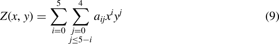
A simple function is a multivariate polynomial, its geometric features are smooth, and it can fit the surface features well. Therefore, a polynomial function is used to fit the deformed surface of the TWS in this study work. The polynomial equation is as follows:
The quality of surface fitting is generally evaluated by the R-squared (R2) parameter. This statistical parameter is defined as the ratio between the regression sum of squares and the total sum of squares. The R2 is calculated by:
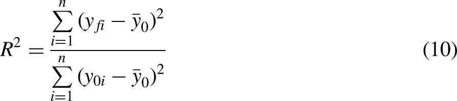
The R2 value represents the overall quality of fit of the data. It can be observed in Eqs. (10) that R2 has a normal value range of [0,1], in which a value closer to one represents a stronger ability of the equation to reflect the value of
Generally speaking, the requirement for good correlation is that R2 is greater than 0.9. In order to generate a polynomial fitting function that can not only fit the deformed surface well but also ensure that the calculation is not too complicated, the highest powers of x and y are determined to be 5 and 4 respectively to fit the surface. The process of data point extraction and multivariate polynomial function fitting of the deformed curved surface of a TWS is shown in Figure 6. The value of R2 is 0.9714, and the fitting results show that the function fits the characteristics of the deformed surface well. Therefore, the function coefficient
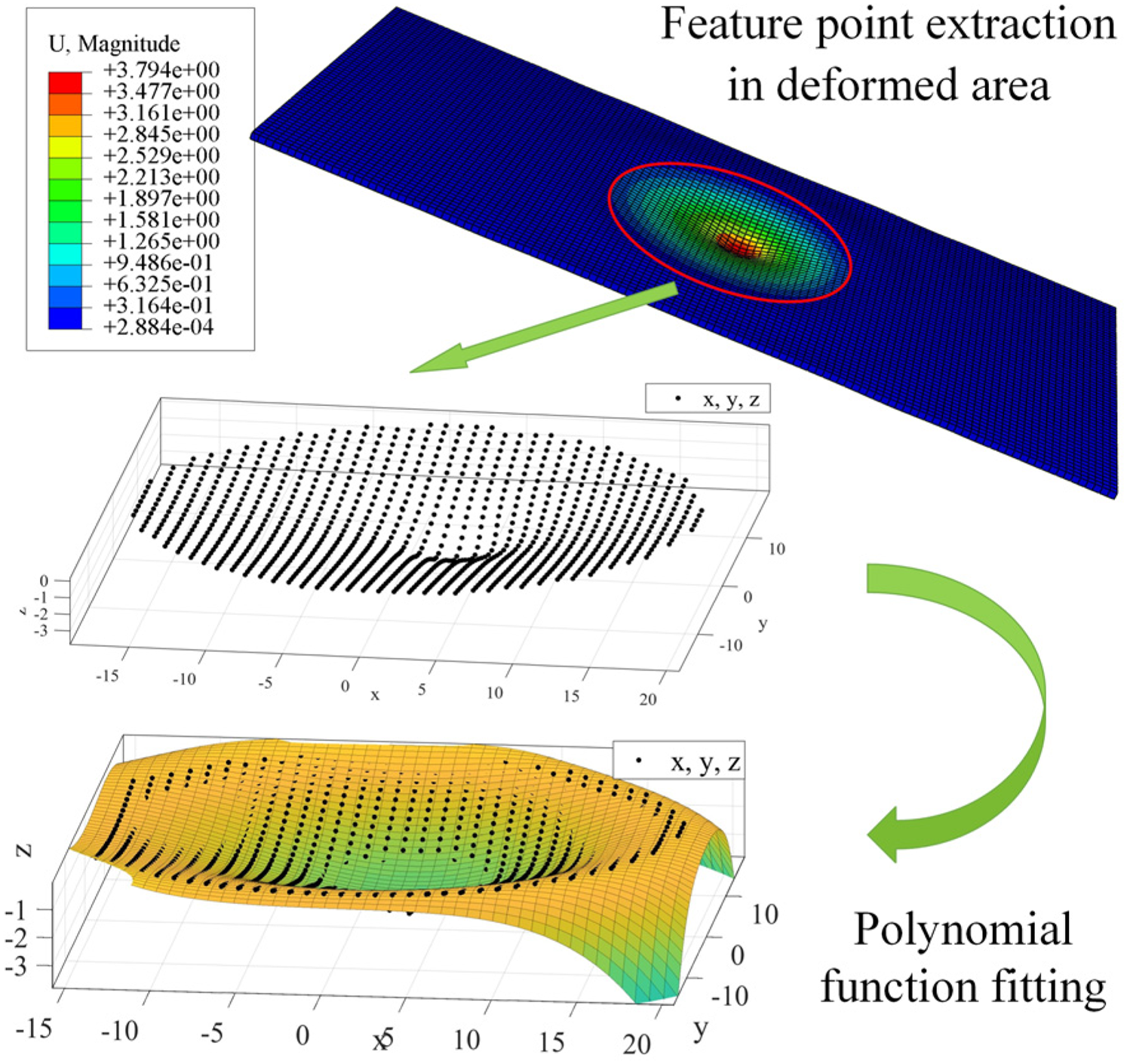
Example of multivariate polynomial function fitting the deformed surface of the TWS.
Data collection
In this study work, we adopted the finite element method to collect the data needed for training and testing to verify the effectiveness of the algorithm, which can save a lot of cost The main details of the FEM and data collection methods are described in this section.
FEM of the TWS
In this study, the FEM of the research object is established that the structure of the TWS is plastic deformation by impact. The FEM of the TWS and the rigid ball were developed by the commercial software ABAQUS, as shown in Figure 7. The TWS was modeled by using the C3D8R element, which is an eight-node linear hexahedral element. For the TWS, the refined mesh size was 1 mm, the coarser mesh size was 4 mm, which results in a total number of 16113 nodes and 10652 elements. For the rigid ball, the total number of nodes and elements are 3021 and 2883, respectively. The thickness of the TWS is T = 1 mm, the length B = 120 mm, and the width A = 60 mm. The large deformation area was concentrated near the impact position in the process of impact deformation. In order to save time and ensure accuracy, we have refined the grid in the impact area and coarsened the grid in the non-impact area.

FEM of the TWS subjected to rigid ball impact.
The reference point is added at the center of the sphere during the impact simulation process, as shown in Figure 7. Then, the rigid ball with some initial velocity
Constitutive modeling
The 7000 series aluminum alloys were widely used in the military and aviation fields of frame, landing gear, hydraulic system and other components, which have the advantages of light weight, high strength, and good workability.37–39 The 7075-T651 aluminum alloy is one of the highest strength aluminum alloys, with high fracture toughness and low fatigue crack growth, durability, strength comparable to steel, and excellent fatigue strength and workability. 40 Therefore, the 7075-T651 aluminum alloy was used as the material in this study for simulation and sample data was collected.
The Johnson-Cook (J-C) model can more accurately simulate the flow stress and thermodynamic state of the metal during plastic deformation, such as strain rate, pressure, temperature, etc. Therefore, the J-C model was used to characterize the constitutive relationship of 7075-T651 aluminum alloy in this study work. The function is described as
41
:

J-C model parameters of 7075-T651 aluminum alloy.

The J-C fracture equation
43
follows the equivalent plastic strain failure criterion, which takes into account strain, strain rate, temperature and pressure. The equivalent plastic strain at the element integration point is considered as the main factor in the J-C dynamic failure model, which is represented by the failure parameter 
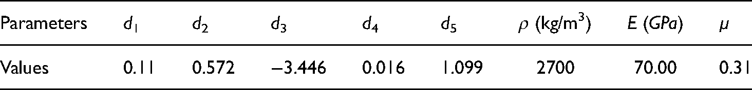
The strain at failure 
The failure parameters in Eqs. (13) are the material parameters determined by the FEM iteratively. The material parameter density
J-C failure model and other parameters of 7075-T651 aluminum alloy.
Boundary and loading conditions
The two ends of the TWS are fixed and restrained, and the rigid ball is completely released from the restraint, giving the rigid ball a specific initial velocity, as shown in Figure 7. Moreover, according to the principle of symmetry, the sampling point of the impact position

Initial impact position of the training data collection.
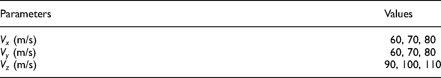
Impact load velocity of the training data collection.
Parametric modeling
In order to simplify the modeling process and improve efficiency, the commercial software ABAQUS was re-developed using Pyhton program, and the batch calculation and data processing of 729 sample models were realized. In the process of parametric modeling, the variables (impact position

Parametric modeling process for simulation of impact deformation of the TWS.
Algorithm implementation
In this study, 729 samples were divided into 27 groups according to different impact speeds, with 27 samples in each group, and the k-fold cross-validation method was used, as shown in Figure 10. Two groups of samples were taken as the test set, in which one duplicate sample was removed, the test data group 1 was used as the test of the extended neural network, with a total of 26 samples, and the test data group 2 was used as the test of the prediction neural network, with a total of 27 samples. The remaining 676 samples serve as the initial training set for the extended neural network.

The k-fold cross-validation to collect training samples.
Training and testing of extended PSO-BP neural network
In this study, 676 training samples and 26 test samples are used to train and test the extended neural network. According to the method described in Section 3. First, the 4-layer PSO-BP neural network model is established, with the impact position and velocity as the input parameters, and the coefficients of the shape fitting function after the deformation of the collision plate was used as the output parameters. The number of nodes in the input layer and output layer are 5 and 20, respectively. And the number of nodes in the two hidden layers are 16 and 22, respectively. Then, the hyper-parameters of the extended PSO-BP neural network model are listed in Table 4. At the same time, we use the early stop callback to stop the training of the neural network. The set standard is: when the MSE reaches a certain value, continue to iterate for 50 steps, and stop the training when the MSE value does not decrease. Finally, the network model is trained. The minimum error is 0.0085035 when iterating 185 steps. The training history of the PSO-BP neural network is shown in Figures 11. In addition, the extended BP neural network model was trained with the same network parameters for comparison, and the training process is shown in Figure 12. The minimum error is 0.0092519 when iterating 153 steps. The results show that the fitting accuracy of the PSO-BP neural network model is higher than that of the BP neural network model, but the training steps are increased.

Training process of the extended PSO-BP neural network.

Training process of the extended BP neural network.
Hyper-parameters of the extended PSO-BP neural network.

The relative error (RE) and the mean relative error (MRE) between the prediction function coefficients of the test set and the actual fitting function coefficients were calculated after the model training is completed. The definitions of RE and MRE are:
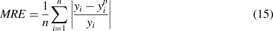
For the 26 samples in test data set 1, the maximum RE predicted with the PSO-BP neural network was 10.91%, and the MRE was 4.35%, while the maximum RE predicted with the BP neural network was 12.05%, and the MRE was 8.17%. The results have shown that the extended PSO-BP neural network model has a better prediction effect on the test and can be used for sample expansion.
Extended PSO-BP neural network is used to expand the sample
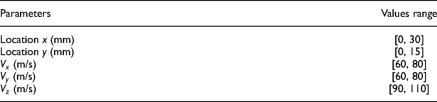
The above results show that the predictive PSO-BP neural network model training has a good fitting effect and can be used for the expansion of the sample database. When sampling using the LHS method, the numerical range of the impact position
Range of position and velocity parameters.
Training and testing of the predictive PSO-BP neural network
The total of 2702 sample sets, including the above-mentioned expanded 2000 sample sets and the original original 676 training samples and 26 test samples, are used as the training set of the predictive PSO-BP neural network model. The 27 samples of the test data set 2 extracted by the k-fold cross-validation method are used as the test set. According to the method described in Section 3. First, the 4-layer PSO-BP neural network model is established, with the coefficients of the shape fitting function after the deformation of the collision plate was used as the output parameters, and the impact position and velocity as the input parameters. The number of nodes in the input layer and output layer are 20 and 5, respectively. And the number of nodes in the two hidden layers are 26 and 24, respectively. Then, the hyper-parameters of the predictive PSO-BP neural network model are listed in Table 6. At the same time, we use an early stop callback to stop the training of the neural network, setting the same criteria as extended PSO-BP neural network. Finally, the network model is trained. The training history of the predictive PSO-BP neural network is shown in Figures 13. The minimum error is 0.011347 when iterating 1045 steps. In addition, the predictive BP neural network model was trained with the same network parameters for comparison, and the training process is shown in Figure 14. The minimum error is 0.060332 when iterating 190 steps. The results show that the fitting accuracy of the PSO-BP neural network model is higher than that of the BP neural network model, but the training steps are increased.

Training process of the predictive PSO-BP neural network.

Training process of the predictive BP neural network.
Hyper-parameters of the predictive PSO-BP neural network.

The actual value of the impact position

Comparison of the actual impact position, the predicted position of BP neural network and the predicted position of PSO-BP neural network and their prediction errors. a) comparison of impact location; b) comparison of prediction errors in the x-coordinate direction; c) comparison of prediction errors in the y-coordinate direction.
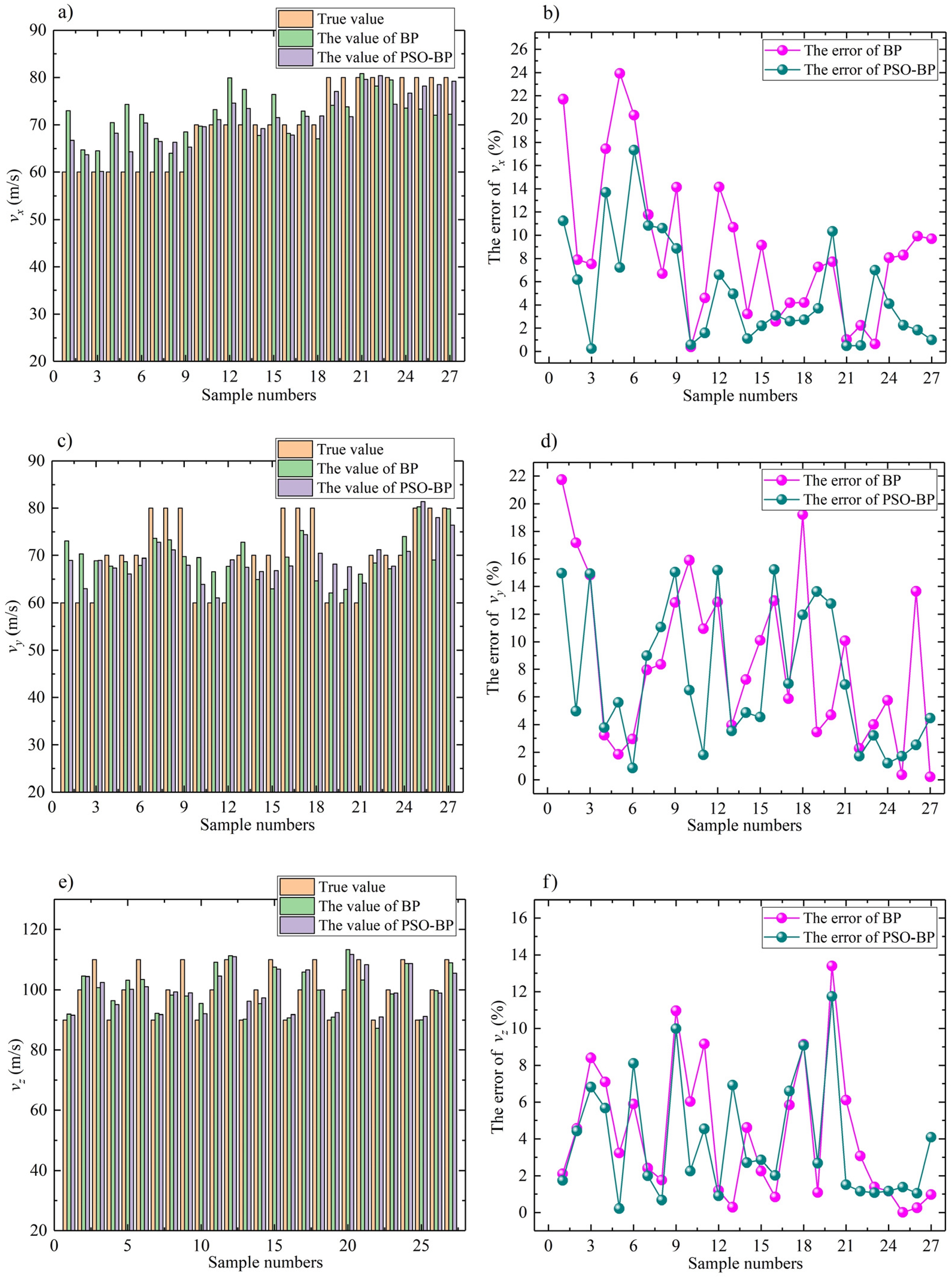
Comparison of the actual impact velocity, the impact velocity of the BP neural network model and the impact velocity of the PSO-BP neural network model and their prediction errors. a) comparison of speed
Conclusions
In this study work, we proposed a PSO-BP neural network method for identifying the impact load condition of the TWS damage based on the principle of reverse engineering. This method was used to solve the engineering inverse problem of identifying the impact position and velocity of plastic deformation damage caused by TWS. Initially, the extended PSO-BP neural network is used 557 sets of known impact position and velocity sample data to construct the relationship between them and the related deformation. This relationship was described by the function coefficients of the multivariate polynomial fitting the three-dimensional deformation surface of the TWS. In particular, multivariate polynomial function was used to fit the deformed feature information of the TWS, and the coefficients were extracted as training data, which greatly reduces the amount of sample data and improves the training efficiency of the model. Then, the training sample set was expanded by 2000 items based on the LHS. Finally, the predictive PSO-BP neural network was trained, and the impact position and velocity were predicted based on the known functional coefficients of the deformed surface. The predicted impact position and velocity are compared with the analysis results of the FEM, which verifies the validity of the algorithm prediction. In addition, we compare the results of the traditional BP neural network model with the results of the PSO-BP neural network model, which proves that the latter has higher prediction accuracy.
The research results show that we have proposed an effective new method, which accurately identifies the impact load conditions of the plastic deformation damage of the TWS. Further expansion, the use of the identified impact information for the inversion of the structural failure process can not only help engineers repair damaged structures, but also help designers improve product design quality. This method has important application value in engineering. It should be noted that although the neural network technology is used to predict the collision position, it has a high accuracy. However, we need to be aware that neural network-based prediction methods also have limitations such as underfitting, overfitting, and overtraining. In future research, these limitations need to be further addressed so that neural network methods can be better applied to engineering.
Footnotes
Author contributions
Jinyu Gu and Yongdang Chen were responsible for the design and implementation of the experimental scheme of the article. Jinyu Gu was responsible for completing the article. Xinxin Song was responsible for data extraction. Xinxin Song was involved in the discussion and significantly contributed to making the final draft of the article. Yongdang Chen was responsible for the revision of the article. All the authors read and approved the final manuscript.
Competing interests
The authors declared no potential conflicts of interest with respect to the research, authorship, and publication of this article.
Ethical approval
Not applicable.
Consent to participate
Not applicable.
Consent to publish
Not applicable.
Funding
The authors disclosed receipt of the following financial support for the research, authorship, and/or publication of this article: Authors gratefully appreciate the support of Xi’an key laboratory of modern intelligent textile equipment (2019220614SYS021CG043).