Experimental investigation of the tip leakage flow in a low-speed multistage axial compressor

Abstract

Casing pressure measurements and Stereoscopic Particle-Image Velocimetry (SPIV) measurements are used together to characterize the behavior of the rotor tip leakage flow at both the design and near-stall conditions in a low-speed multistage axial compressor. A three-dimensional Navier-Stokes solver is also performed for the multistage compressor and the prediction of tip leakage flow is compared with SPIV data and casing dynamic static pressure data. During the experiment 10 high-frequency Kulite transducers are mounted in the outer casing of the rotor 3 to investigate the complex flow near the compressor casing and Fourier analyses of the dynamic static pressure on the casing of the rotor 3 are carried out to investigate the tip leakage flow characteristics. At the same time, the two CCD cameras are arranged at the same side of the laser light sheet, which is suitable for investigating unsteady tip leakage flow in the multistage axial compressor. The SPIV measurements identify that the tip leakage flow exists in the rotor passage. The influence of tip leakage flow leads to the existence of low axial velocity region in the rotor passage and the alternating regions of positive and negative radial velocity indicates the emergence of tip leakage vortex (TLV). The trajectory of the tip leakage vortex moves from the suction surface toward the pressure surface of adjacent blade, which is aligned close to the rotor at the design point (DP). However, the tip leakage vortex becomes unstable and breaks down at the near-stall point (NS), making the vortex trajectory move upstream in the rotor passage and causing a large blockage in the middle of the passage.

Introduction

In axial compressor, tip leakage flow is caused by the pressure difference between blade suction surface and pressure surface. The leakage flow in tip area interacts with the main flow near the suction surface of the blade, and then rolls up into the tip leakage vortex. Previous studies have shown that tip flows, especially tip leakage vortex, play an important role in compressor aerodynamic stability. In addition, tip leakage flow is the main source of aerodynamic noise in compressor. For the above reasons, the generation and development of rotor tip leakage vortices and the relationship between tip leakage vortices and compressor loss and instability have become the focus of the research.^1–3 As discussed by Denton, the challenges of modeling tip leakage flow in turbomachinery are critical. ⁴ However, the current computational fluid dynamics (CFD) techniques applied to the multistage compressor design are based on Reynolds-averaged Navier-Stokes (RANS) method, ignoring the fluctuation information in the flow field, which cannot adequately simulate the tip leakage flow. Although Detached Eddy Simulation (DES) and Large Eddy Simulation (LES) methods are good choices to simulate tip leakage vortices, more computational resources and time are required to perform multistage full-annulus compressor simulations. Therefore, experimental method is still a useful and appropriate path to investigate tip leakage flow in multistage axial compressors.

In previous researches, dynamic pressure transducers have been mounted on the outer casing to investigate unsteady tip leakage flow in the compressor.^5–7 The leakage flow trajectory across the blade passage can be identified by the low pressure region near the outer casing. However, the flow structures below the casing cannot be acquired by the pressure transducers, which need to be measured by the reliable method for understanding the behavior of rotor tip leakage vortex.

Compared with Hot Wire Anemometry and Laser Doppler velocimetry (LDV), the Particle-Image Velocimetry (PIV) technique overcomes the disadvantages of point-based tool and is able to capture spatial characteristics. The flow structures and unsteady characteristics of tip leakage flow can be analyzed by using PIV technique. In recent decades, researchers have used PIV technique to investigate unsteady tip flows in axial compressors.^8–11 To sum up, simultaneous casing pressure measurements and the PIV measurements can provide significant insight into the unsteady flow characteristics of the tip leakage vortex and the interaction between the tip leakage vortex and surrounding fluid. In this paper, the behaviors of the rotor tip leakage flow at both the design and near-stall conditions are investigated in Nanjing University of Aeronautics and Astronautics 4-stage large-scale low-speed research compressor.

Low-speed axial compressor

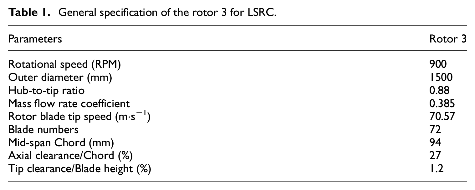
Figure 1 shows the schematic drawing of compressor test rig at Nanjing University of Aeronautics and Astronautics (NUAA). The low-speed research compressor is a large-scale axial compressor with four approximately repeating stages, which is applied to low-speed model testing (LSMT). The third stage of the compressor is the model stage, while the first two stages and the last stage respectively provide suitable upstream and downstream environment. The information of axial compressor can be referred to the previous articles.^12,13 Considering the existence of flow separation at the hub corner for the rotor and stator of stage 3, several useful blading improvement techniques were employed on the stage 3 to improve compressor performance. Additional information about the improvement method is available in the references.^14,15 In this paper, measurements are performed in the optimized third-stage rotor passage (Rotor 3) of the multistage axial compressor at the design point (mass flow rate coefficient is 0.385) and the near-stall point (mass flow rate coefficient is 0.34), respectively. For the rotor conditions presented herein, the general specifications are listed in Table 1. Figure 2 shows the front and side view of the rotor 3.

Figure 1.

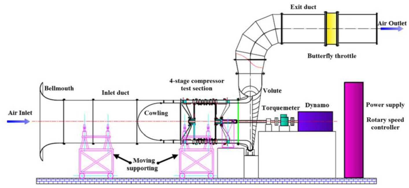
Schematic drawing of compressor test rig.

Table 1.

General specification of the rotor 3 for LSRC.

Parameters	Rotor 3
Rotational speed (RPM)	900
Outer diameter (mm)	1500
Hub-to-tip ratio	0.88
Mass flow rate coefficient	0.385
Rotor blade tip speed (m·s−1)	70.57
Blade numbers	72
Mid-span Chord (mm)	94
Axial clearance/Chord (%)	27
Tip clearance/Blade height (%)	1.2

Figure 2.

Front and side view of the compressor rotor 3.

Test facility

Casing-mounted pressure transducers

A large amount of flow blockage and aerodynamic loss are likely to occur near the compressor casing, and compressor stall is closely related to flows in the endwall area. In order to deeply investigate the complex flow characteristics near the compressor casing, 10 high-frequency Kulite Mic-062-LG transducers are mounted in the outer casing of the rotor 3. The sensors are axially spaced each 6 mm covering rotor axial chord from −8.5% to 110.8%. The specific relative location of the sensors are listed in Table 2. The sensor positions mounted on the outer casing are shown in Figure 3.

Table 2.

Distributions of the pressure tansducers sensor-array.

	Axial chord (x/c)	Probe number
Casing-mounted unsteady static pressure of Rotor 3	−8.5%	CH1
	4.8%	CH2
	18.0%	CH3
	31.3%	CH4
	44.5%	CH5
	57.8%	CH6
	71.0%	CH7
	84.3%	CH8
	97.6%	CH9
	110.8%	CH10

Figure 3.

Sketch map of the dynamic pressure transducers.

SPIV setup and data processing

SPIV optical system

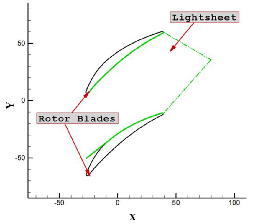
The SPIV system used in this paper is the product of TSI Incorporation. The SPIV system consists of laser system, CCD cameras, and control system (including data collection and post-processing). Nd:YAG laser is used as the light source and the illumination energy is 35 mJ/pulse at a 15 Hz repetition rate. Two CCD cameras with 1024×1024 pixels are positioned on the same side of the laser light sheet. For SPIV measurement, two high-speed CMOS cameras with a certain deflection Angle are used for shooting, and then the 3d spatial calibration data is used to process the image to obtain the velocity components in three directions in the plane. Compared to the PIV technology, SPIV can obtain the velocity component out of the plane. ¹⁶ The installation locations of high-speed CMOS camera and the light sheet periscope probe are shown in Figure 4. In order to introduce the laser beam into the passage of rotor 3, the light sheet periscope probe is inserted in the middle of the passage of the stator 3. The angle of incidence of the beam is close to the blade stagger angle, which prompt the beam to lighten the entire rotor passage to the maximum. The light sheet is parallel to the access window and the illuminated region is located in the access window, so two CCD cameras can record clear image data.

Figure 4.

Installation of the SPIV system in the compressor.

Flow seeding

In the SPIV measurement, the particle dispersion device adopts two PIV experimental particle generators provided by TSI Incorporation. DEHS particles were used as tracer particles for measurement, which had good scattering property, large production, and harmless to human body and environment. DEHS particles are used as tracer particles for measurement, which have good scattering property, large production, and harmless to human body and environment. The particle size of the generated particles is about 1.5 μm, and the diameter distribution is relatively uniform, which is very suitable for the measurement of complex flow field in multistage axial compressor. The particle generator begins to propagate in the far front of the experimental bench. After the particles are diffused, they are inhaled into the compressor through the trumpet mouth at the front of the experimental bench, and particles with appropriate density and uniform distribution are formed in the target area of the rotor passage.

Data acquisition and processing

Since the compressor rotor is a rotating part, this paper makes use of the phase-locked trigger device to make the frequency of the measured rotor blade passage through the measurement window the same as the laser pulse emission frequency of the SPIV system, and controls the phase difference between the two, so as to realize the image acquisition in the rotor blade passage by the SPIV system. By adjusting the depth of the light sheet probe inserted into the casing and the angle of light, the flow field information of different blade spans can be measured. Figure 5 shows the layout of the measurement sections and the relative span locations of SPIV test section are listed in Table 3. The optical path simulation at one location in rotor blade is presented in Figure 6. In the process of SPIV measurement, the system parameters are reasonably set to minimize the system error and ensure the measurement accuracy. At least 100 groups of velocity field photos at different moments are acquired for each measured plane and each rotor phase, then cross-correlation analysis is carried out for each group of photos to obtain the instantaneous velocity field. Finally, the instantaneous velocity field at each moment is averaged to obtain the time average velocity field. In data processing, the images are analyzed with a multi-pass process. The interrogation windows adopted successively are 32 pixels × 32 pixels and 16 pixels × 16 pixels respectively. In this case, the random error of the SPIV measurement is small.

Figure 5.

Schematic layout of test sections.

Table 3.

The relative span locations of SPIV measured section.

Section number	1	2	3	4	5	6	7
Relative span (r/R)	70%	75%	80%	85%	90%	95%	97%

Figure 6.

Maps of optical path simulation in rotor blade.

CFD prediction of tip leakage flow

Fully three-dimensional Navier-Stokes flow solver EURANUS is used for steady single-passage calculation. Considering the multistage environment, the object of numerical simulation is a four-stage low-speed compressor. Detailed turbulence model, grid distribution and solution method can be found in the previous paper. ¹⁵ In order to improve the orthogonality of the blade surface mesh, O4H and butterfly topologies are adopted in the main flow area and the rotor tip clearance gap, respectively. The mesh for the rotor had 73 nodes in the radial direction, and 17 nodes are given in the radial direction of the tip clearance gap to ensure accurate simulation of tip clearance flow. In the numerical simulation, the flow coefficients corresponding to the design point and the near-stall point are 0.385 and 0.34. The rotor tip leakage vortex trajectory and the interface between tip leakage flow and main flow are obtained by numerical calculation, and the flow structure of tip leakage flow in tip clearance is analyzed. CFD prediction of tip leakage flow will be compared with SPIV data and casing dynamic static pressure data.

Results and discussion

Overall performance

The measured pressure rise of the 4-stage compressor and the stage 3 are shown in Figures 7 and 8. The abscissa axis represents the mass flow rate coefficient, and the ordinate axis represents the total-total pressure rise coefficient, which is defined here as: ψ_tt = (P^*₃−P^*₁) / (0.5ρU_m²), and the mass flow rate coefficient is defined as: ϕ = V_z/ U_m, where V_z is the axial velocity, U_m is the midspan rotational speed, P^* is the total pressure and subscript 1 and 3 represent the stage inlet and outlet planes, or compressor inlet and outlet planes, respectively. The mass flow coefficient of design point is 0.385, as indicated by the dash-pink line. Rotation stall occurs below the flow coefficient of 0.319.

Figure 7.

Pressure rise of the entire 4-stage compressor.

Figure 8.

Pressure rise of the stage 3.

Unsteady pressure measurements on the rotor casing

Figure 9 shows the contours of the static pressure coefficient on the rotor casing at different working conditions (design point and near-stall point). The static pressure coefficient here is calculated with the following equation: C_p = (P_s−P₀) / (0.5ρU_tip²), for which P_s denotes the ensemble-averaged static pressure in 20 rotor revolutions, P₀ denotes the atmospheric pressure, and U_tip is the blade tip speed. The static pressure contours in the figure is obtained by first converting the voltage signals of 10 dynamic pressure sensors into pressure signals, and then converting the pressure signal over time into the pressure signal along the space. The conversion process confirms that the flow field in the rotor is periodic unsteadiness. Figure 10 shows the comparison of casing static pressure contour for the measurement results and CFD prediction. It is generally believed that the minimum static pressure point corresponds to the initial position of tip leakage vortex on the suction surface of the blade. As the flow coefficient decreases, the initial point of tip leakage vortex moves forward. Some high or low pressure areas different from other periods appear in the figure, which may be caused by the deviation in blade processing or not completely periodic unsteadiness of the rotor tip flow.

Figure 9.

Maps of measured casing static pressure distributions at the design and near-stall conditions.

Figure 10.

Comparison of casing static pressure contour for the measurement results (left) and CFD prediction (right) at the design and near-stall conditions.

Figure 11 presents the contours of the ensemble-averaged root mean square value for static pressure coefficient on the rotor casing at design and near-stall point. It can be seen that there is a certain high RMS value area at different working conditions, which corresponds to the influence region of the tip leakage flow. The static pressure troughs marked by black lines are deemed as the trajectories of tip leakage flow. As the flow coefficient decreases, the trajectory of tip leakage flow moves toward the leading edge plane and the width of the high RMS region is gradually shortened, indicating that tip leakage vortex mixes with the main flow drastically within a shorter distance and dissipates rapidly. In addition, with the decrease of mass flow coefficient, the fluctuation amplitude of the tip leakage vortex of rotor 3 gradually decreases.

Figure 11.

Measured casing static pressure root mean squre value at the (a) design and (b) near-stall conditions.

Figure 12 shows the spectrum of casing static pressure at the design and near-stall conditions. The abscissa axis represents the relative axial position, and the ordinate axis represents the frequency. The contours represent the amplitude of all pressure signals at the corresponding axial position and frequency by fast Fourier transformation (FFT), which reflects the energy amplitude of a frequency signal. There is a long and narrow region with a frequency value close to 1080 Hz in the Figure 12(a), which represents the blade pass frequency (BPF) signal. With the loading increases, the BPF signal always has a large energy amplitude at near-stall point. In addition, there exists a wide frequency region with a high amplitude, which is represented by a black dotted rectangle in each figure. Figure 12(b) shows that the high amplitude region moves toward the leading edge at near-stall point. According to the analysis by Inoue et al., ¹⁷ the turbulence intensity and wall pressure fluctuation behind the interface between the incoming flow and the tip leakage flow are more significant than other regions not affected by the tip leakage vortex. Therefore, the forward movement of the high amplitude region at near-stall condition indicates the strong interaction between the main flow and the tip leakage flow and the forward movement of the interface between the incoming flow and the tip leakage flow.

Figure 12.

Spectrum of casing static pressure at the (a) design and (b) near-stall condition.

Unsteady flow in the rotor tip region from SPIV measurement

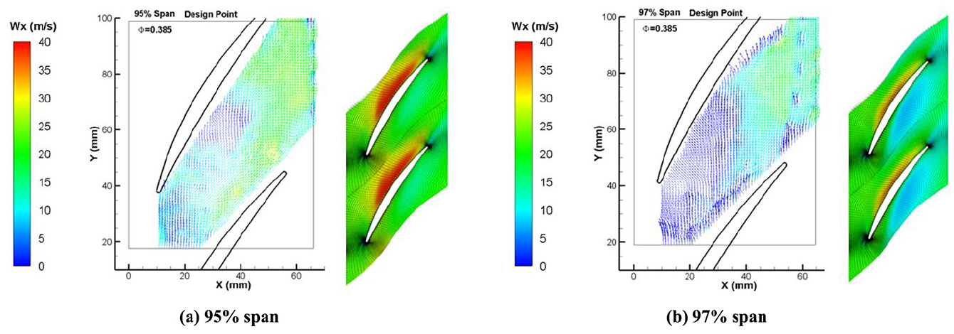
SPIV flow measurements are obtained at design point and near-stall point for rotor 3. The SPIV date are obtained at seven span locations from 70% to 97 span. Considering the flow field below 90% span is less affected by tip leakage flow (not presented here), the phase-locked ensemble-averaged relative velocity at different spans are shown in Figure 13, which are 90%, 95% and 97%span respectively. The x-coordinate represents the axial direction, y-coordinate represents the circumferential direction, and the vector color represents the magnitude of the in-plane relative velocity. Due to the deviation of the cameras from the direction perpendicular to the rotor passage during the measurement, the view range of the measurement is blocked by the neighboring rotor blade, making it impossible to get the detailed velocity vectors at the near suction surface. In addition, due to the position of the cameras, it is affected by the reflection on the blade surface, so there are some blind spots near the pressure surface. Figure 13 presents that the relative velocity of each section decreases from the throat to the trailing edge gradually at the design point and near-stall point, which objectively reflects the process of fluid deceleration and diffusion in the rotor blade passage. As depicted in figure, the regions affected by tip leakage flow have low velocity and the leakage flow moves from the blade suction toward the adjacent blade pressure surface, and the low-speed region appears along the direction of the leakage flow. At near-stall point, the low-speed region moves upstream and the trajectory of tip leakage vortex moves closer to the leading edge plane and the flow tends to overflow from the leading edge of the adjacent blade, which increases the passage blockage area and loss rapidly.

Figure 13.

Measured in-plane relative velocity vectors and streamlines from 90% to 97% span at the design and near-stall condition.

The comparison of axial velocity for the SPIV measurement and CFD calculation at 95% and 97% span at the design point illustrates that there is an obvious low axial velocity region in the rear part of the rotor passage under the influence of tip leakage flow shown in Figure 14. Due to the blocking of the light path, the SPIV experiment failed to detect the flow field near the suction surface of the rotor.

Figure 14.

Comparison of axial velocity for the SPIV experiment (left) and CFD calculation (right) at the design point.

In order to further capture the trajectory of the tip leakage vortex, Figures 15 and 16 show the comparison of radial velocity for SPIV measurement and CFD results at three spans under the conditions of design point and near stall point respectively. In the SPIV diagram, the color of velocity vector represents the radial velocity magnitude, in which the radial outward direction is defined as positive and the radial inward direction is defined as negative. The alternating red and blue regions (black dotted boxes) in the figure are considered to be the locations and extent of the tip leakage vortex. The comparison of the experiment and CFD leakage vortex trajectories shows good consistency at three blade spans. It can be seen from the figure that with the decrease of flow rate, the rotor tip leakage flow becomes more active. The change of the position of the red/ blue regions in the rear part of the rotor blade indicates the oscillation and breakage of the tip leakage vortex.

Figure 15.

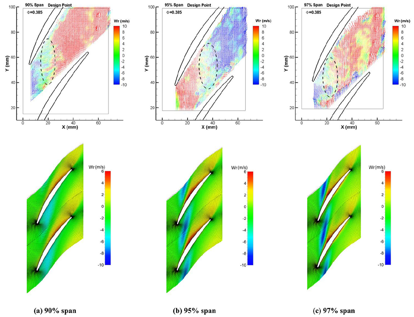
Comparison of radial velocity for SPIV experiment (top) and CFD calculation (bottom) from 90% to 97% span at design point.

Figure 16.

Comparison of radial velocity for SPIV experiment (top) and CFD calculation (bottom) from 90% to 97% span at near-stall point.

Figure 17(a) shows the visualization of the TLV trajectory at 97% span for rotor 3 at design point. Four transient particle images from t1 to t4 describe the development of the tip leakage flow, with a fluctuation period of about 0.002 s. The leakage flow trajectory in the figure changes with time, which illustrate the movement of tip leakage vortex is an unsteady process. The tip leakage vortex is generated at t1 and enters a stable development stage at t2. Then, the tip leakage vortex enters the instability stage, swaying and splitting in the process of moving downstream at t3. Finally, the tip leakage vortex mixes with the main flow and leaves the blade passage at t4.

Figure 17.

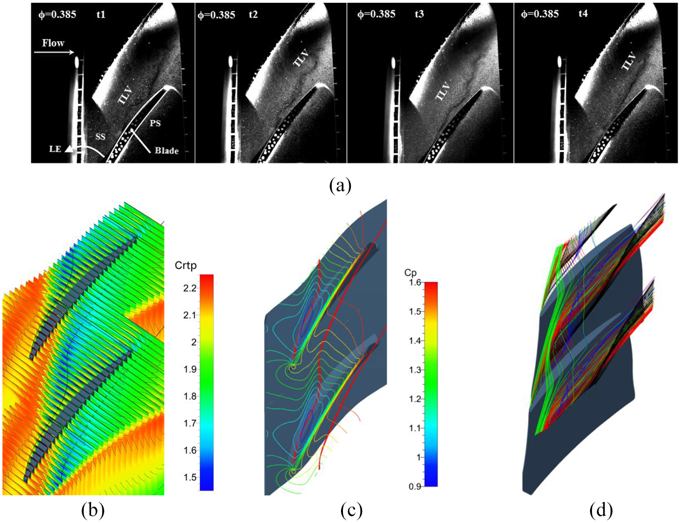
Comparison of TLV trajectory for SPIV experiment (top) and CFD calculation (bottom) at the design point. (a) Visualization of the TLV trajectory at 97% span for rotor 3, (b) relative total pressure contour, (c) static pressure coefficient isoline, and (d) rotor tip clearance streamlines.

Figure 17(b–d) show the characteristics of the leakage vortex obtained by CFD calculation. Figure 4(b) shows the dimensionless relative total pressure contour and the tip leakage vortex trajectory (black line) in the rotor passage at design point. The relative total pressure coefficient here is calculated with the following equation: C_rtp = (P_rtp−P₀) / (0.5ρU_tip²), for which P_rtp denotes the local relative total pressure, P₀ denotes the atmospheric pressure, and U_tip is the blade tip speed. Relative total pressure loss occurs in the region passed by the tip leakage vortex in the figure. As the tip leakage vortex moves downstream, the range of the high-loss region expands radially and circumferentially. It can be speculated that tip leakage vortex starts from about 20% chord and the influence region occupies about 60% passage area in the circumferential direction at design point. The blue loss region disappears after 80% chord due to its own expansion and strong mixing with the mainstream and the trajectory of the tip leakage vortex is also consistent with the experimental results. Figure 16(c) shows the isoline distribution of static pressure coefficient on the rotor casing at the design point. The streamlines from leading edge of the rotor is basically fitted to the static pressure troughs on the rotor casing, which indicates that there is an obvious static pressure loss in the area covered by the tip leakage vortex. Figure 16(d) shows the comparison of tip leading edge streamlines at four different heights in rotor tip clearance, which further illustrates the flow structure of leakage flow in tip clearance. The four positions at different heights are 0.35 h (blue), 0.5 h (black), 0.625 h (red) and 0.75 h (green), respectively, where h is the tip clearance size, so 0 h and 1 h represent the blade tip and casing positions. As shown in the figure, the flow from the rotor leading edge will be sucked up into tip leakage vortex in the tip region below 0.625 h, and with the increase of height, the position occupied by tip leakage vortex expands from inside to outside. In the tip region above 0.625 h, the fluid flowing out of the leading edge of the rotor will not be sucked into a blade tip leakage vortex, but is more prone to secondary leakage.

Figures 18 and 19 show the measured instaneous relative velocity vector vectors and streamlines for rotor 3 at 97% span at the design and near-stall condition, respectively. During the experiment, the rotor position has been phase locked, so the change of tip leakage vortex position relative to the rotor can be clearly seen from the figures. The unsteady motion of tip leakage vortex causes the streamlines change constantly with time. As the flow rate decreases, tip leakage vortex become unstable, which breaks into many small streamwise vortices. The position and strength of streamwise vortices change at different times, resulting in the larger low-speed regions and more complicated streamlines. The interaction between the concentrated tip leakage vortex and the fluid at leading edge is enhanced at near-stall point, because the interface between tip leakage flow and the main flow is close to the leading edge plane, which is consistent with the conclusion of the over-rotor static pressure contours.

Figure 18.

Measured instantaneous relative velocity vectors at 97% span for rotor 3 at design condition.

Figure 19.

Measured instaneous relative velocity vectors and streamlines at 97% span for compressor rotor at near-stall condition.

Conclusion

In this paper, casing pressure measurement and SPIV measurements have been successfully conducted in the test of multistage low-speed axial compressor at NUAA. The static pressure distribution on the rotor casing and detailed velocity fields in rotor tip region have been analyzed to characterize the behaviors of the rotor tip leakage flow at both the design and near-stall conditions. A three-dimensional Navier-Stokes solver has shown good agreement with the experimental results in many aspects of tip leakage flow, including static pressure field and tip velocity vector field. The following conclusions are drawn:

The static pressure contours show that the regions with high RMS value of static pressure coefficient are affected by tip leakage flow. The trajectory of the leakage flow can be tracked by the locus of the static pressure troughs. With the decrease of mass flow coefficient, the trajectory of tip leakage flow moves to the leading edge of blade.

The Fourier analysis of the pressure signal shows that the BPF signal always has a large energy amplitude at different working conditions. There exists a wide frequency region with a high amplitude on the spectrum map and the forward movement of the high amplitude region at near-stall condition indicates the strong interaction between the main flow and the tip leakage flow.

The SPIV measurements reconstruct the velocity field in the rotor passage. The alternating regions of positive and negative radial velocity indicate the existence of leakage flow and can be considered as tip leakage vortex. Tip leakage vortex trajectory starts from about 20% chord and the influence region occupies about 60% passage area in the circumferential direction at design point. The high loss region disappears after 80% chord due to its own expansion and strong mixing with the mainstream at design point. The streamlines from leading edge of the rotor is basically fitted to the static pressure troughs on the rotor casing, which indicates that there is an obvious static pressure loss in the area covered by the tip leakage vortex. The flow from the rotor leading edge will be sucked up into tip leakage vortex in the tip region below 0.625 h. However, the fluid flowing out of the leading edge of the rotor will not be sucked into a blade tip leakage vortex, but is more prone to secondary leakage in the tip region above 0.625 h. The development of tip leakage vortex is unstable and can be divided into four stages: generation, stable development, swaying and splitting, and finally mixing with the mainstream. At the near-stall point, the leakage vortex is extremely unstable and breaks up into small streamwise vortices. The interface between the leakage vortex and the main flow is parallel to the leading edge plane, producing a larger blockage region.