Sage Journals: Discover world-class research

Abstract

Non-destructive analysis of fiber reinforced polymer (FRP) composites is important for confirming the long-term safety and durability of concrete structures. In this study, a pulse-heating infrared thermography technique was used to detect and characterize bonding defects of externally bonded carbon fiber reinforced polymers (CFRP) on concrete surface structures. The CFRP composite contains various bonding defects of three different sizes located at five different depths. Sequential thermal images were obtained to describe the temperature contrast and shapes of the bonding defects. Through analysis of the maximum temperature response, we investigated the effects of defect size and depth on the defect temperature response. The relationship between the defect depth and maximum temperature response was used to quantitatively estimate the defect depth. In addition, finite element simulations were performed on the CFRP composites with bonding defects to investigate the temperature response of various defects, which showed good agreement with the experimental results. This confirms the effectiveness of the infrared thermography method to detect and characterize bonding defects of FRP composites bonded on concrete structures.

Keywords

Infrared thermography bonding defect pulse-heating temperature response CFRP

Introduction

Fiber reinforced polymer (FRP), which are light weight, strong, and corrosion resistant, are widely used in civil engineering. Among applications of FRP, they are commonly used to externally reinforce concrete structures. Meier et al.¹ investigated carbon FRP (CFRP) plate reinforced concrete beams in 1982 at the Swiss Federal Laboratories for Materials Science and Technology. The American Concrete Institute has issued guidelines which specify design criteria, installation procedures, and acceptance criteria for externally bonded FRP systems for strengthening concrete structures.² The interfaces between the concrete surface and the FRP layer, or between two adjacent FRP layers rely on epoxy resin for transferring stress. This structure requires non-destructive evaluation to ensure durability and long-term performance of the FRP reinforcements.

Commonly used visual inspection and hammering methods can only determine the existence of defects inside a structure but cannot give information on the size and depth of defects.³ Ultrasonic testing has been used to detect CFRP defects, and offers advantages in terms of rapid scan speed, good resolution and flaw detection capabilities, and the ability for use in the field. However, owing to the limitations of the test surface and the need for multi-point data, the application scope of this method is limited.⁴ Microwave testing, based on a type of radar wave detection, is simple and can rapidly generate radar (SAR) tomography images of CFRPs for analysis; however, these techniques, require improvements in overall image quality, particularly spatial and temporal resolution.⁵ X-ray computed tomography qualitatively and quantitatively detects defects in CFRPs and gives insight into their 3D shape and properties; however, the instrumental demands make it difficult to apply this method in large-scale engineering.⁶ Here, we use infrared thermography (IRT) as a nondestructive evaluation tool for identifying and characterizing defects in FRP/concrete interfaces or between layers of FRPs.^7–9

Pulse-heating infrared thermography is a non-destructive detection method that uses high-energy flash lamps to apply thermal excitation to the measured object. Internal defects of the object are exposed as having different surface temperature distributions. An infrared thermal camera is used to continuously measure the surface temperature field. The obtained sequence of thermal images is processed and analyzed to realize qualitative and quantitative analysis of internal defects.^10–14 In aerospace structures, this technique has been applied for many years, particularly for detection and characterization of delamination in carbon/epoxy composites.¹⁵ The application of this method in detection of FRP strengthened concrete elements has also started to receive attention in recent years.^16,17 Recently, scholars have used pulse infrared thermography inspection to conduct a series of experimental and numerical simulation studies on the interface of FRP-reinforced concrete structure, including the heating method of FRP defect detection, the effect of thermal excitation energy on defect detection, the influence of environment on defect detection, the location of FRP layer defect, the defect detection of FRP components in the process of static loading, composite defect detection under fatigue loading, defect detection in actual FRP structural engineering and other aspects.^18–26 However, applications of infrared thermography to concrete structures are at an early stage of development and further experimental and numerical studies are needed.

In this study, the pulse-heating infrared thermography method was adopted on the CFRP sheets strengthened concrete slab. The surface temperature change was continuously observed and recorded by the infrared thermal camera. The relationships between the size, depth of the defect and the temperature response were analyzed. Moreover, the maximum temperature response was introduced to quantitatively characterize the defect depth. The results were verified by the finite element simulation.

Test material and specimen fabrication

A concrete slab (500 mm × 400 mm × 80 mm) was manufactured and externally strengthened by five superimposed layers of CFRP sheets with intermediate glue layers. We used reinforced CFRP sheets (UT70-20 carbon fiber sheet, FAW: 200 g/m², Toray Industries, Inc.). The glue layers were an epoxy resin and curing agent, produced by Shanghai Sanyou Co. and uniformly mixed at a ratio of 2:1. Bonding defects were simulated by replacing the adhesive material by polyethylene foam, which has thermal conductivity similar to those of air. The polyethylene foam has good insulation properties, low density, high stability, and is better able to simulate defects in practical engineering. The bonding defects were simulated by square foam flakes with a thickness of approximately 1 mm and areas of 900, 400, and 100 mm², respectively (Figure 1). These defects were placed either between the concrete surface and the lower CFRP sheet, or between two adjacent CFRP sheets. Bonding defects with different conditions and specimen photo are shown in Figure 2. According to their depths in the composite surface, these defects were classified into five categories denoted as A, B, C, D, and E. Defects in category A were subdivided into A1, A2 and A3 depending on their different sizes. The final specimen contained defects of three different sizes located at five different depths.

Figure 1.

Bonding defects based on polyethylene foam.

Figure 2.

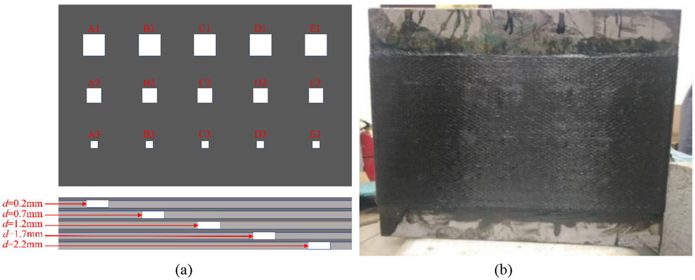
Bonding defects with different conditions. (a) Location and number of different bonding defects. (b) Specimen photo.

To ensure the bonding quality, the concrete slab was first ground and cleaned. Protrusions of the surface were removed with a concrete grinder. Indentations were filled with cement, ground with sandpaper and the smoothed surface was then cleaned by wiping with alcohol. Then the adhesives (a mixture of epoxy resin and curing agent) were evenly applied to the surface of the concrete slab with a brush. The bonding defects and CFRP sheet were pasted to the corresponding position coated with adhesive. Next, a roller was moved across the fiber sheet until there were no air bubbles between the concrete and fiber sheet. The following layers were applied until five layers of CFRP sheets and the corresponding bonding defects were all pasted. Finally, the specimen was cured for 7 days at room temperature (20 + 0.5°C).

Test equipment and methods

For the tests, Fluke Tix620 infrared thermal camera and thermal excitation device are the main equipment. The infrared thermal camera produces images of 640 × 480 pixels in the frequency of 30 Hz in the view field of 32.7° × 24.0°at the temperature range of −40°C to +600°C with the accuracy of ±2°C or ±2% of reading. The thermal sensitivity is ≺40 mK @ +30°C and the spectral response was between 7.5 and 14 μm. For the thermal excitation device, two high-energy halogen lamps with the flash frequency of 50 Hz and the power of 1000 W per halogen lamp were adopted in the tests. Moreover, a time controller was equipped to control the excitation start and the excitation interval.

The pulse-heating infrared thermography method was applied to the specimen. The surface of the specimen was heated with two high-energy halogen lamps that thermally excited an area of approximately 0.02 m² at a fixed relative distance of approximately 0.6 m. The time controller set the pulse interval of the lamps to be 15 s. In accordance with the start of thermal heating, the infrared thermal camera operated to visualize the temperature of the specimen surface in the time interval of 240 s with the images of 640 × 480 pixels. The camera was connected to a computer and data were directly transferred to a computer for storage and processing.

Analysis of sequential thermal image

Sequential thermal images of the specimen acquired after the pulse-heating stage are shown in Figure 3a. To improve defect imaging, Principal Component Analysis (PCA) technique could be considered to perform dimension reduction on the original thermal images. The PCA image reconstructed by the first 20 principal components extracted from original images is shown in Figure 3b, in which cumulative explained variance reaches more than 99%. Through PCA technique, the redundancy in the images could be reduced and the amount of information could be compressed into fewer features. The number and position of the defects were consistent with the placement, as shown in Figure 2a. For the bonding defects numbered A1 to E1 with an area of 900 mm², it can be noted that with the increase of the defect depth, the defect temperature decreases, the temperature contrast between the defective and non-defective area reduces and even becomes difficult to be distinguished. On the other hand, the increase in defect depth also causes the edge blurring of the defective area. For example, the rectangular features of the defect A1 are quite obvious, while the geometric features of the defect E1 are almost indistinguishable. For the bonding defects numbered A2 to E2 with an area of 400 mm², there are similar rule to the former defect group of A1 to E1. As the defect depth increases, the temperature contrast decreases and area edges become increasingly blurred. The rectangular outlines of defects D2 and E2 have been difficult to be recognized. The third group of defects A3 to E3 has the lower temperature contrast and more poorly defined edge features than the inferred two defect groups, which may cause large errors in analysis.

Figure 3.

Sequential thermal image of the specimen after the pulse-heating interval of 15s. (a) Original thermal image. (b) Thermal image proceeded by PCA.

Analysis of defect depth and defect size based on temperature response

In infrared thermography inspection, sequential thermal images obtained by an infrared thermal camera represent the real-time temperature distribution of the specimen surface. To qualitatively or quantitatively analyze defects, we selected thermal images at the maximum temperature response ΔT(t). This specific image can be obtained based on the temperature response—time curve. The temperature response ΔT(t) is expressed by:

Δ T (t) = T_{d} (t) - T_{s} (t),

(1)

where t is time and T_d(t) and T_s(t) represent the mean temperature of the defective area and non-defective area at time t, respectively.

As presented in Figure 4, in the sequential thermal images, the defective area and non-defective area correspond to different temperature data sets, and the values of each pixel are the real-time temperatures at those points. By calculating the average of all pixels over a particular area, we obtain the mean temperature of that area, that is, T_d(t) and T_s(t). To reduce the calculation error, many pixels (more than 1000) were averaged over each area.

Figure 4.

Temperature of defective and non-defective area in sequential thermal image.

Depending on the various defect sizes, the bonding defects were divided into three groups, successively numbered (A1-E1), (A2-E2) and (A3-E3). On the basis of the above method, the temperature response—time curves of each group were calculated, as shown in Figure 5.

Figure 5.

Temperature response−time curves of various defects. Defects areas of (a) 900 mm²; (b) 400 mm²; (c) 100 mm².

As demonstrated in Figure 5, defects of different sizes at the same depth reached their maximum temperature response at the same time. Larger defects showed a higher maximum temperature response and there was a decrease in the maximum temperature response of the defects A1, A2, and A3 as the defect size decreased.

All the defects reached their maximum temperature response in the heat dissipation phase after external heating, whereas the time to reach the maximum temperature response varied depending on the defect depths. This result is similar to that reported by Taillade et al.²⁷ As the defect depth increased, the maximum temperature response was delayed. We consider the first group of A1 to E1 as an example. The time difference to reach the maximum temperature response between the defects A1 and E1 was approximately 20 s. Conversely, for deep defects, a higher maximum temperature response was achieved, as indicated in Figure 5. This will be helpful to clearly observe the defects in lower depth. Moreover, for defects of lower depth, the temperature rises faster in the heating process and the time to reach the maximum temperature response is shorter. During the heat dissipation phase after external heating, the temperature drops also faster and then reaches a lower surface temperature in the end.

Thus, we conclude that the temperature response of the defect is related to the defect depth. In this study, there were 15 bonding defects of three different sizes at five different depths (Figure 2a). The defects were also divided into three groups of (A1-E1), (A2-E2), and (A3-E3) according to the defect size for investigating the correlation between the defect depth and the maximum temperature response, as illustrated in Figure 6.

Figure 6.

Relationship of maximum temperature response and defect depth.

It can be noted that the defect depth is exponentially related to the maximum temperature response with the same defect size:

d = m \exp (n Δ T) + l

(2)

where d is the defect depth, m, n and l are the fitting parameters in the tests. The detailed values are listed in Table 1.

Table 1.

Fitting parameters in tests.

Defect size (mm²)	m (mm)	n	l (mm)
900	5.92	−0.46	−0.14
400	4.14	−0.40	−0.41
100	4.43	−0.60	−0.32

The defect depth dependence of the maximum temperature response was the same for defects having different areas; however, the variation of the main parameters m, n, and l was not monotonic. For example, the parameter m had its smallest value at the middle of the 400 mm² defect, which means that as the defect size increased, m first decreased and then increased with the value changing from 5.92 to 4.14 and then to 4.43. The changes of parameter l followed a similar pattern to those of m. However, the parameter n had the opposite behavior to that of m. The value of n first decreased and then increased for smaller defects. The fitting degrees of the three curves were all greater than 0.96, which confirmed the regularity of the data.

The temperature response obtained from the pulse-heating infrared thermography suggested that it is possible to determine the defect depth with good accuracy by formula (2) with the introduction of the maximum temperature response. This feature would enable quantitative characterization of the defect depth. However, more test data are needed to verify the performance of this method, which will be obtained in our future studies.

Comparison of finite element simulation and test results

The thermal conduction analysis on the concrete slab reinforced by CFRP sheets with bonding defects subjected to an external heat pulse was carried out. The variation of the surface temperature responses of the 15 defects of different sizes and depths under heating and heat dissipation processes was investigated by simulations. Here, we assume that the thermal stress was uniformly applied over the composite surface. The physical model used the same geometric parameters as the experimental specimens. The thermodynamic parameters of various materials in the finite element simulation are given in Table 2. To better compare with the test results, the thermal conductivity of polyethylene foam used as the bonding defects in test was adopted for computer simulations. If there exist other defects in practical engineering, it is needed to select the proper thermal conductivity to match with the actual defects.

Table 2.

Thermodynamic parameters of various materials.

Materials	Thermal conductivity (W/m·K)	Density(kg/m³)	Specific Heat Capacity (J/(kg°C))
CFRP sheet	X-axis:8.9	1760	720
	Y-axis:2.9
	Z-axis:2.9
epoxy resin	0.22	1960	1870
polyethylene foam	≤0.037	50	540
concrete	1.28	2360	970

In the simulation, the concrete slab was divided by Solid70 element, which has a 3-D thermal conduction capability. The element has eight nodes with a single degree of freedom, temperature, at each node. The surface mesh was firstly drawn and then stretched to obtain the three-dimensional mesh. The mesh adopted a transitional form. With the change of the temperature gradient, the mesh closer to the CFRP cloth surface became denser. The composite layup of CFRP cloth and epoxy resin was in Shell131 element. Shell131 is a 3-D layered shell element with thermal conduction capability in the plane and thickness direction. Each shell owns 4 nodes, which is suitable for steady and transient thermal analysis of 3-D shell elements. The CFRP cloth and epoxy resin were crosswise arranged, and the anisotropy of the thermal conductivity of CFRP cloth was considered. For unidirectional fiber cloth, the greater thermal conductivity was existed along the fiber distribution direction.

The simulation was performed by applying temperature loading and heat flow loading. In order to correspond to the laboratory environment, the initial temperature was selected according to the laboratory experiment. The field variable of the transient temperature field is ϕ (x, y, z, t). It is known that the temperature of the fluid medium in contact with the object and the convective heat transfer coefficient are both of 10W/m²· s. The boundary conditions satisfy Equation 3:

k_{x} \frac{\partial ϕ}{\partial x} n_{x} + k_{y} \frac{\partial ϕ}{\partial y} n_{y} + k_{z} \frac{\partial ϕ}{\partial z} n_{z} = h (ϕ_{a} - ϕ)

(3)

where, t is time, k_x, k_y, k_z are the thermal conductivity of the material along the three main directions (W/m·K), n_x, n_y, n_z is the cosine of the outside normal direction of the boundary, h is the convective heat transfer coefficient, ϕ_a It is the ambient temperature under natural convection.

The whole solution process was divided into two loading steps, namely the heating process and the cooling (chrill-down) process. In the first loading step, a convective loading was applied on the back of the model, and a thermal convective loading was applied on the front of the model, which was also the surface of the CFRP reinforcement layer. The second loading step was to remove the surface heat flow, and convective loadings were applied on the back and front of the model. The calculated model and the obtained temperature nephogram after a pulse-heating are shown in Figure 7. The temperature response of the defects was not sufficiently clear at the end of the pulse-heating.

Figure 7.

Finite element simulation results. (a) Calculated model. (b) Temperature nephogram after the pulse-heating at 15-s intervals.

Through the use of these finite element simulations, we determined the maximum temperature response of each defect and the time to reach the maximum temperature response. The maximum temperature response curves at different defect depths are plotted in Figure 8.

Figure 8.

Comparison between simulation and test results of temperature response-defect depth.

It can be demonstrated that the maximum temperature response reaches at a certain point in the heat dissipation process, which is consistent with the rule in the test results. There was a slight difference between the simulation data and the test results, which we attribute to the parameters used in the simulation differing somewhat from those of the actual experimental materials. Furthermore, in the simulation, thermal stress was uniformly applied to the composite surface, negating the effects of uneven heating. Moreover, in the tests, the details for example, the uneven conglutination of CFRP sheets or unevenly cut of defect all will cause the error increase, while these problems will be avoided in simulation with the more regular data. Overall, there was only a small difference between the simulation and experimental results, indicating that the simulation provides a reasonable estimate of the experimental behavior.

Conclusions

In this paper, pulse-heating infrared thermography was developed to investigate the nondestructive evaluation of CFRP composite applied to concrete. On the basis of sequential thermal images obtained from pulse-heating infrared thermography, the temperature contrast and geometric features of bonding defects with three different sizes located at five different depths were described. Moreover, through the introduction of the temperature response, the effects of defect size and defect depth on the parameters such as real-time temperature and maximum temperature response were analyzed in a qualitative way. The embedded bonding defects and delamination generated in the externally bonded CFRP-concrete composites were characterized by infrared thermography. A further theoretical analysis of the relationship between the defect depth and the maximum temperature response contributed to quantitative retrieval of the defect depth. Finite element simulations of the concrete slab reinforced by CFRP sheets with bonding defects subjected to an external heat pulse were conducted to study the surface temperature response of various defects with different sizes and depths in heating to heat dissipation process. There is good agreement between the simulation data and test results despite slight differences between the model and experimental sample; hence, the simulation provides a robust estimate of the experimental behavior. In conclusion, infrared thermography offers a simple and effective method for non-destructive evaluation of FRP strengthening bonded on concrete structures. In future studies, we will perform additional testing to confirm the validity of this approach and extend the applicability. Further tests on various shapes, bonding defect materials, and FRP materials should be performed to fully interpret results of infrared thermography.

Footnotes

Declaration of conflicting interests

The author(s) declared no potential conflicts of interest with respect to the research, authorship, and/or publication of this article.

Funding

The author(s) disclosed receipt of the following financial support for the research, authorship, and/or publication of this article: This work was supported by the National Key Research and Development Program of China (No. 2017YFC0805900); Innovative Venture Technology Investment Project of Hunan Province (2018GK5028); open fund of National Engineering Research Center on Diagnosis and Rehabilitation of Industrial Building (No.2016YZAKy01); the National Natural Science Foundation of China (No. 51578140); a Project Funded by the Priority Academic Program Development of Jiangsu Higher Education Institutions (PAPD, No. CE02-2-8); Postgraduate Research & Innovation Program of Jiangsu Province and Fundamental Research Funds for Southeast University (No. KYLX15_0084).

ORCID iD

Bo Wen

References

Meier

. Strengthening of structures using carbon fibre/epoxy composites. Constr Build Mater 1995; 9: 341–351.

ACI 440.2R-02. Guide for the design and construction of externally bonded FRP systems for strengthening concrete structures. Reported by ACI Committee 440. 2002. American Concrete Institute.

Galietti

Luprano

Nenna

, et al. Non-destructive defect characterization of concrete structures reinforced by means of FRP. Infrared Phys Technol 2007; 49: 218–223.

Ray

Hasan

Clegg

. Evaluation of defects in FRP composites by NDT techniques. J Reinf Plast Comp 2007; 26: 1187–1192.

Sutthaweekula

Tian

Wang

, et al. Microwave open-ended waveguide for detection and characterisation of FBHs in coated GFRP pipes. Compos Struct 2019; 225: 111080.

Katunin

Dańczak

Kostka

. Automated identification and classification of internal defects in composite structures using computed tomography and 3D wavelet analysis. Arch Civ Mech Eng 2015; 15: 436–448.

Tian

Malekmohammadi

, et al. New features for delamination depth evaluation in carbon fiber reinforced plastic materials using eddy current pulse-compression thermography. NDT E Int 2019; 102: 264–273.

Lai

Kou

Poon

, et al. Characterization of the deterioration of externally bonded CFRP-concrete composites using quantitative infrared thermography. Cement Concrete Comp 2010; 32: 740–746.

Valluzzi

Grinzato

Pellegrino

, et al. IR thermography for interface analysis of FRP laminates externally bonded to RC beams. Mater Struct 2009; 42: 25–34.

10.

Azenha

Faria

Figueiras

. Thermography as a technique for monitoring early age temperatures of hardening concrete. Constr Build Mater 2011; 25: 4232–4240.

11.

Ghiassi

Silva

Oliveira

, et al. FRP-to-Masonry Bond Durability Assessment with Infrared Thermography Method. J Nondestruct Eval 2014; 33: 427–437.

12.

Konstantopoulos

Tonejc

Maier

, et al. Exploiting temperature measurements for cure monitoring of FRP composites–applications with thermocouples and infrared thermography. J Reinf Plast Comp 2015; 34: 1015–1026.

13.

Hiasa

Birgul

Catbas

. Investigation of effective utilization of infrared thermography (IRT) through advanced finite element modelling. Constr Build Mater 2017; 150: 295–309.

14.

Omar

Nehdi

Zayed

. Infrared thermography model for automated detection of delamination in RC bridge decks. Constr Build Mater 2018; 168: 313–327.

15.

Katunin

Dragan

Dziendzikowski

. Damage identification in aircraft composite structures: a case study using various non-destructive testing techniques. Compos Struct 2015; 127: 1–9.

16.

Brown

Hamilton

. Quantitative infrared thermography inspection for FRP applied to concrete using single pixel analysis. Constr Build Mater 2013; 38: 1292–1302.

17.

Brown

Hamilton

. Heating methods and detection limits for infrared thermography inspection of fiber-reinforced polymer composites. ACI Mater J 2007; 104: 481–490.

18.

Toubal

Karama

Lorrain

. Damage evolution and infrared thermography in woven composite laminates under fatigue loading. Int J Fatigue 2006; 28: 1867–1872.

19.

Schmutzler

Garcia

Sato

, et al. Influence of delamination characteristics in carbon fibre/epoxy laminates on signal features of pulse thermography. J Nondestruct Eval 2015; 34: 5.

20.

Lai

Kou

Poon

, et al. Effects of elevated water temperatures on interfacial delaminations, failure modes and shear strength in externally-bonded CFRP-concrete beams using infrared thermography, gray-scale images and direct shear test. Constr Build Mater 2009; 23: 3152–3160.

21.

Levar

Hamilton

. Nondestructive evaluation of carbon fiber-reinforced polymer-concrete bond using infrared thermography. ACI Mater J 2003; 100: 63–72.

22.

Noszczyk

Nowa

. Inverse contrast in non-destructive materials research by using active thermography. Materials 2019; 12: 835.

23.

Théroux

Dumoulin

Maladague

. Square heating applied to shearography and active infrared thermography measurements coupling: from feasibility test in laboratory to numerical study of pultruded CFRP plates glued on concrete specimen. Strain 2014; 50: 404–416.

24.

Mabrouki

Genest

Shi

, et al. Numerical modeling for thermographic inspection of fiber metal laminates. NDT E Int 2009; 42: 581–588.

25.

Halabe

Vasudevan

Klinkhachorn

, et al. Detection of subsurface defects in fiber reinforced polymer composite bridge decks using digital infrared thermography. Nondestruct Test Eva 2007; 22: 155–175.

26.

Fernandes

Sena-Cruz

Xavier

, et al. Durability of bond in NSM CFRP-concrete systems under different environmental conditions. Compos Part B-Eng 2018; 138: 19–34.

27.

Taillade

Quiertant

Benzarti

, et al. Shearography and pulsed stimulated infrared thermography applied to a nondestructive evaluation of FRP strengthening systems bonded on concrete structures. Constr Build Mater 2011; 25: 568–574.

Pulse-heating infrared thermography inspection of bonding defects on carbon fiber reinforced polymer composites

Abstract

Keywords

Introduction

Test material and specimen fabrication

Test equipment and methods

Analysis of sequential thermal image

Analysis of defect depth and defect size based on temperature response

Comparison of finite element simulation and test results

Conclusions

Footnotes

Declaration of conflicting interests

Funding

ORCID iD

References