Sage Journals: Discover world-class research

Abstract

Distributed electric drive technology has become an important trend because of its ability to enhance the dynamic performance of multi-axle heavy vehicle. This article presents a joint estimation of vehicle’s state and parameters based on the dual unscented Kalman filter. First, a 12-degrees-of-freedom dynamic model of an 8 × 8 distributed electric vehicle is established. Considering the dynamic variation of some key parameters for heavy vehicle, a real-time parameter estimator is introduced, based on which simultaneous estimation of vehicle’s state and parameters is implemented under the dual unscented Kalman filter framework. Simulation results show that the dual unscented Kalman filter estimator has a high estimation accuracy for multi-axle distributed electric vehicle’s state and key parameters. Therefore, it is reliable for vehicle dynamics control without the influence of unknown or varying parameters.

Keywords

Multi-axle distributed electric vehicle state estimation parameter estimation dual unscented Kalman filter co-simulation

Introduction

The application of distributed drive technology in heavy vehicle could bring greater benefits than passenger car. Since the clutch, transmission, transfer case, differential, drive shaft, and other mechanical components are removed, it simplifies the vehicle structure and makes its layout more convenient. In addition, each wheel is controlled by the wheel hub motor independently to increase the vehicle’s maneuverability. However, the degree of freedom (DOF) of vehicle control increases significantly with the number of axle. Vehicle dynamics control is enhanced if the real-time and accurate acquisition of vehicle state and key parameters is achieved.^1,2 Therefore, for the multi-axle distributed electric vehicle, it is important to estimate the state which is expensive or difficult to measure, or the parameter which is unknown or variable.

The vehicle state can be estimated by kinematic-based methods and dynamic-based methods. The former involve direct integral method for measurements, which is subject to cumulative error,^3,4 whereas the latter are more often used for vehicle state estimation because of the higher accuracy even if based on low-cost sensors. The typical algorithms include Kalman filter, particle filter, sliding-mode observer, Luenberger observer, and so on.^5–9 To date, the nonlinear Kalman filter provides a prospective method for the nonlinear vehicle system, including the extended Kalman filter (EKF) algorithm and the unscented Kalman filter (UKF) algorithm.^10–12 Sebsadji et al.¹³ and Dakhlallah et al.¹⁴ used the EKF method to estimate the longitudinal velocity, lateral velocity, and yaw rate. On the basis of this method, estimation of road gradient, road friction coefficient, and vehicle sideslip angle is achieved. Best et al.¹⁵ proposed the adaptive EKF to estimate the tire force, which improves the accuracy due to the change in the tire-cornering stiffness. In Antonov et al.,¹⁶ an UKF algorithm was used to estimate tire slip and vehicle slip angle based on magic formula and bicycle model. In Doumiati et al.,¹⁷ UKF and EKF were proposed and compared to address system nonlinearities and unmodeled dynamics. Experimental results demonstrate that the two approaches could provide accurate estimations for calculating lateral tire force and vehicle sideslip angle. However, UKF has better second-order accuracy than EKF and reduces the amount of computation without Jacobian matrices.

The UKF method relies on the vehicle dynamics model. Compared to those of the traditional vehicle, the dynamic characteristics of the distributed electric vehicle are obviously different. One of the characteristics of the latter is that the driving torque of each wheel can be obtained timely by the wheel hub motor. In addition, it brings new requirements for the estimation of vehicle longitudinal speed and road surface, since no wheel is nondriving wheel. In Geng et al.,¹⁸ a fuzzy estimator was adopted for the sideslip angle of four-wheel distributed electric vehicle. In Gu et al.,¹⁹ the longitudinal velocity, lateral velocity, and yaw rate of a four-wheel drive-by-wire vehicle are estimated based on the UKF algorithm and a 7-DOF model. Nam et al.²⁰ used the EKF algorithm to estimate the sideslip angle and tire cornering stiffness simultaneously for the distributed electric vehicle.

Some vehicle parameters such as the position of mass center, vehicle mass, and yaw moment of inertia may change during the different driving conditions, especially for multi-axle heavy vehicle. This change of key parameters would affect the accuracy of state estimator, which is established based on fixed parameters. Therefore, the estimation of vehicle parameters needs to be introduced for the unknown and varying parameters. With the advantage of mutual correction, some traditional vehicles have started using the joint estimator of state and parameters. Wenzel et al.²¹ used two EKFs in parallel to reduce the effect of varying vehicle parameters. In Li et al.,²² the estimation of vehicle state and road friction coefficient based on dual-capacity Kalman filter was proposed. The bench test shows that it has better estimation accuracy than dual EKF. Considering the precision and real time, a dual unscented Kalman filter (DUKF) estimator for the multi-axle distributed electric vehicle is designed in this article. It is an important prerequisite for future vehicle dynamics control.

The remainder of this article is organized as follows. Section “Modeling of multi-axle distributed electric vehicle” introduces a vehicle dynamics model suitable for estimation. Section “DUKF algorithm” gives an overview of the DUKF algorithm and then details the design for joint estimator of state and parameters based on multi-axle distributed electric vehicle. Section “Simulation and analysis” gives the simulation results under double lane change (DLC) test and sinusoidal input of steering wheel test. Conclusions and future work are presented in section “Conclusion.”

Modeling of multi-axle distributed electric vehicle

Modeling overview

Real-time and accurate acquisition of vehicle’s lateral and rollover state is important in modeling. The main characteristic of the distributed electric vehicle is the use of electric wheel, which brings the challenge for estimation. For example, longitudinal velocity cannot be achieved directly since each wheel is the driving wheel. In addition, the driving torque of each wheel is easy to measure through the torque of motor.

In this article, we look to estimate eight states which represent vehicle’s motion stability and three key parameters for an 8 × 8 distributed electric vehicle. The vehicle model is established as shown in Figure 1. O-xyz is the vehicle-based coordinate system, u is the longitudinal velocity along the x-axis, v is the lateral velocity along the y-axis, w is the vertical velocity of the sprung mass centroid along the z-axis, r is the yaw rate around the z-axis, p is the roll rate around the x-axis, and q is the pitch rate around the y-axis. The longitudinal force, lateral force, and vertical force of each wheel are represented by F_xi, F_yi, and F_zi (i = 1, 2, …, 8), respectively. L₁ is the distance from the first axis to the second axle, L₂ is the distance from the center of mass to the second axle, L₃ is the distance between centroid and the third axle, L₄ is the distance from the third axle to the fourth axle, and B is the wheel track. Besides, some parameters are not shown in the figure, including Ψ, the yaw angle; Φ, the roll angle, θ, the pitch angle; and β, the sideslip angle. The height of the mass center and the distance from the mass center to the roll axis are represented by h and h′, respectively.

Figure 1.

The model of an 8 × 8 distributed electric vehicle.

Vehicle dynamics

To represent the vehicle states of planar/rollover stability effectively, a 12-DOF model is adopted, including longitudinal motion, lateral motion, yaw motion, roll motion, and rotary motion of eight wheels. The equation governing its dynamics is expressed as

{\begin{matrix} \overset{\cdot}{u} = a_{x} + rv \\ \overset{\cdot}{v} = a_{y} - ru \\ \overset{\cdot}{r} = M_{z} / I_{zz} \\ \overset{\cdot}{ϕ} = \overset{\cdot}{ϕ} \\ \overset{\cdot\cdot}{ϕ} = \frac{m_{s} gh' \tan ϕ + m_{s} h' a_{y} - K_{ϕ} ϕ - C_{ϕ} \overset{\cdot}{ϕ}}{I_{xxs}} \end{matrix}

(1)

I_{w} \frac{d ω_{i}}{dt} = T_{i} i_{g} - F_{zwi} \cdot f \cdot r_{w} - F_{xwi} r_{w}

(2)

where $ϕ$ is the roll angle, $\overset{\cdot}{ϕ}$ is the roll velocity, $K_{ϕ}$ is the roll stiffness coefficient, and $C_{ϕ}$ is the roll damping coefficient. In addition, a_x and a_y are, respectively, the longitudinal and lateral acceleration and M_z is the yaw moment, which can be obtained by the tire dynamics model as follows

a_{x} = \frac{1}{m} (\begin{matrix} (F_{xw 1} \cos δ_{1 l} - F_{yw 1} \sin δ_{1 l}) + (F_{xw 5} \cos δ_{1 r} - F_{yw 5} \sin δ_{1 r}) \\ + (F_{xw 2} \cos δ_{2 l} - F_{yw 2} \sin δ_{2 l}) + (F_{xw 6} \cos δ_{2 r} - F_{yw 6} \sin δ_{2 r}) \\ + F_{xw 3} + F_{xw 4} + F_{xw 7} + F_{xw 8} \end{matrix})

(3)

a_{y} = \frac{1}{m} (\begin{matrix} (F_{xw 1} \sin δ_{1 l} + F_{yw 1} \cos δ_{1 l}) + (F_{xw 5} \sin δ_{1 r} + F_{yw 5} \cos δ_{1 r}) \\ + (F_{xw 2} \sin δ_{2 l} + F_{yw 2} \cos δ_{2 l}) + (F_{xw 6} \sin δ_{2 r} + F_{yw 6} \cos δ_{2 r}) \\ + F_{yw 3} + F_{yw 4} + F_{yw 7} + F_{yw 8} \end{matrix})

(4)

\begin{matrix} M_{z} = (L_{1} + L_{2}) (F_{xw 1} \sin δ_{1 l} + F_{yw 1} \cos δ_{1 l} + F_{xw 5} \sin δ_{1 r} + F_{yw 5} \cos δ_{1 r}) \\ + L_{2} (F_{xw 2} \sin δ_{2 l} + F_{yw 2} \cos δ_{2 l} + F_{xw 6} \sin δ_{2 r} + F_{yw 6} \cos δ_{2 r}) \\ - L_{3} (F_{yw 3} + F_{yw 7}) - (L_{3} + L_{4}) (F_{yw 4} + F_{yw 8}) + \frac{B}{2} (\sum_{i = 5}^{8} F_{xi} - \sum_{i = 1}^{4} F_{xi}) \end{matrix}

(5)

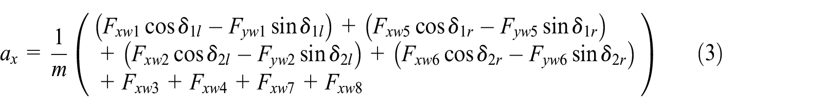
where δ_1l, δ_2r, δ_2l, and δ_2r are the steering angles of the first two axles, respectively. Besides, the sideslip angle β can be calculated by longitudinal speed and lateral speed

β = \arctan \frac{v}{u}

(6)

Tire dynamics

The tire dynamic model contains the longitudinal force module and the lateral force module. Since the motor torque of the electric wheel can be obtained for the distributed electric vehicle, it is different from the conventional vehicle and makes the calculation of the tire’s longitudinal force easier. According to the wheel rotation equation (2), the equation of the tire longitudinal force can be obtained as

F_{xwi} = \frac{(T_{i} i_{g} - I_{w} {\overset{\cdot}{ω}}_{i})}{r_{w}} - F_{zwi} \cdot f

(7)

By contrast, the calculation of the lateral force of tire F_yw is more complicated. An HSRI (Highway Safety Research Institute) tire model²³ is adopted as follows

F_{yw} = {\begin{matrix} - C_{α} \frac{S_{y}}{1 - S_{x}} & L \geq 1 \\ - C_{α} \frac{S_{y}}{1 - S_{x}} L (2 - L) & 0 < L < 1 \\ - C_{s} S_{y} μ F_{zw} {[{C_{s}}^{2} + {(C_{α} S_{y})}^{2}]}^{- 1 / 2} & L = 0 \end{matrix}

(8)

L = \frac{1}{2} μ F_{zw} (1 - S_{x}) {[{(C_{s} S_{x})}^{2} + {(C_{α} S_{y})}^{2}]}^{- 1 / 2}

(9)

where C_s and C_α are the longitudinal and lateral stiffnesses of the tire, respectively; S_x and S_y are the longitudinal slip ratio and lateral slip ratio, respectively; μ is the coefficient of road adhesion; and F_zw is the vertical load of the tire.

The longitudinal slip ratio of tire S_x can be calculated according to equation (10)

λ_{i} = \frac{ω_{i} r_{w} - v_{whi}}{max (ω_{i} r_{w}, v_{whi})}

(10)

where ω_i is the angular rate of each wheel, and the horizontal velocity of the wheel center v_whi can be represented as

v_{whi} = (u \pm \frac{B}{2} r) \cos δ_{i} + (v \pm L_{i} r) \sin δ_{i}

(11)

The lateral slip ratio of tire is a relational expression for the tire slip angle, as shown in equation (12), and the tire slip angle is calculated according to equation (13)

S_{yi} = \tan α_{i}

(12)

α_{i} = δ_{i} - \arctan \frac{v_{wyi}}{v_{wxi}}

(13)

DUKF algorithm

Algorithm overview

Two UKF filters operate individually and simultaneously in DUKF. In this article, the estimator of vehicle state and vehicle parameters exchanges and corrects the information of each other. Both the estimators consist of prediction module, construction of Sigma point module, and correction module. The principle of DUKF is shown in Figure 2.

Figure 2.

The scheme of DUKF.

We assume that the vehicle system can be represented by the following nonlinear discrete system equation

{\begin{matrix} x_{k + 1} = f (x_{k}, u_{k}, θ_{k}) \\ y_{k + 1} = h (x_{k}, u_{k}, θ_{k}) \end{matrix}

(14)

where x and $θ$ are the variables of vehicle state and vehicle parameter, respectively. The specific steps of algorithm are as follows:

1. Initialization

First, the initial values of state vector, parameter vector, covariance of state error, and covariance of parameter error are set as ${\hat{x}}_{0}$ , $P_{x 0}$ , ${\hat{θ}}_{0}$ , and $P_{θ 0}$ , respectively.

2. Parameter prediction

The parameter vector and the covariance of parameter error at time k + 1 are predicted as follows

{\hat{θ}}_{k + 1}^{-} = {\hat{θ}}_{k}

(15)

P_{θ, k + 1}^{-} = P_{θ, k} + Q_{θ}

(16)

where $Q_{θ}$ is the covariance matrix of process noise.

3. Construction of Sigma point of state vector

The symmetric point sampling strategy is used to construct a Sigma point set χ_i of state vector at time k and its weights of first-order and second-order statistical characteristics $W_{x, i}^{m}$ and $W_{x, i}^{c}$

{\begin{matrix} χ_{0, k} = {\hat{x}}_{k} \\ χ_{i, k} = {\hat{x}}_{k} + {(\sqrt{(n_{x} + λ_{x}) P_{x, k}})}_{i} i = 1, 2, \dots, n_{x} \\ χ_{i, k} = {\hat{x}}_{k} - {(\sqrt{(n_{x} + λ_{x}) P_{x, k}})}_{i - n_{x}} i = n_{x} + 1, n_{x} + 2, \dots, 2 n_{x} \end{matrix}

(17)

{\begin{matrix} W_{x, 0}^{m} = \frac{λ_{x}}{n_{x} + λ_{x}} \\ W_{x, i}^{m} = \frac{1}{2 (n_{x} + λ_{x})} i = 1, 2, \dots, 2 n_{x} \end{matrix}

(18)

{\begin{matrix} W_{x, 0}^{c} = \frac{λ_{x}}{n_{x} + λ_{x}} + (1 - α^{2} + β) \\ W_{x, i}^{c} = \frac{1}{2 (n_{x} + λ_{x})} i = 1, 2, \dots, 2 n_{x} \end{matrix}

(19)

where ${\hat{x}}_{k}$ and $P_{x, k}$ are the estimated state vector and the covariance of the state error at time k, respectively; n_x is the dimension of the state vector; and λ_x is the coefficient of the sample point of the state vector, and we have

λ = α^{2} (n + κ) - n

(20)

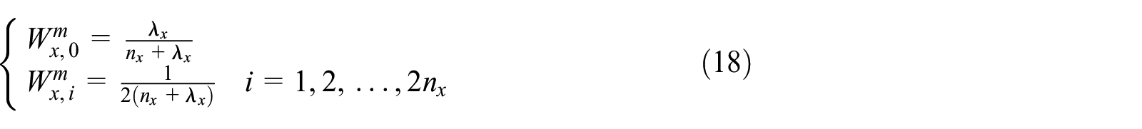
where α is a very small positive number, which we set to 10⁻³, and $κ$ is the second-order coefficient, whose value is 0 when n_x is greater than 3.

4. State prediction

The state prediction contains the prediction of state vector and observation vector. First, the mapping set of points is achieved by transformation of the Sigma point of state vector according to the state equation (14)

χ_{i, k + 1}^{-} = f (χ_{i, k}, u_{k}, {\hat{θ}}_{k + 1}^{-})

(21)

Second, a priori estimation at time k + 1 is obtained by weighting

{\hat{x}}_{k + 1}^{-} = \sum_{i = 0}^{2 n_{x}} W_{x, i}^{m} χ_{i, k + 1}^{-}

(22)

P_{x, k + 1}^{-} = \sum_{i = 0}^{2 n_{x}} W_{x, i}^{c} (χ_{i, k + 1}^{-} - {\hat{x}}^{-}_{k + 1}) {(χ_{i, k + 1}^{-} - {\hat{x}}^{-}_{k + 1})}^{T} + Q_{x}

(23)

Then, this set of points is transformed according to the observation equation (14)

γ_{i, k + 1}^{-} = h (χ_{i, k + 1}^{-}, u_{k + 1}, {\hat{θ}}_{k + 1}^{-})

(24)

Finally, the estimated value of the observation vector at time k + 1 and its covariance are obtained by weighting

{\hat{y}}^{-}_{k + 1} = \sum_{i = 0}^{2 n_{x}} W_{x, i}^{m} γ_{i, k + 1}^{-}

(25)

P_{y, k + 1} = \sum_{i = 0}^{2 n_{x}} W_{x, i}^{c} (γ_{i, k + 1}^{-} - {\hat{y}}^{-}_{k + 1}) {(γ_{i, k + 1}^{-} - {\hat{y}}^{-}_{k + 1})}^{T} + R_{x}

(26)

5. State correction

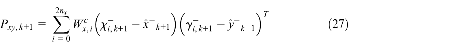
The state correction includes the correction of the state vector and the covariance of the state error. First, the cross-covariance between the state vector and the observation vector is calculated

P_{xy, k + 1} = \sum_{i = 0}^{2 n_{x}} W_{x, i}^{c} (χ_{i, k + 1}^{-} - {\hat{x}}^{-}_{k + 1}) {(γ_{i, k + 1}^{-} - {\hat{y}}^{-}_{k + 1})}^{T}

(27)

Then, the Kalman gain matrix of the state vector is calculated

K_{x, k + 1} = P_{xy, k + 1} P_{y, k + 1}^{- 1}

(28)

Finally, the posterior estimation of the state vector and the covariance of the state error are calculated and updated, respectively

{\hat{x}}_{k + 1} = {\hat{x}}_{k + 1}^{-} + K_{x, k + 1} (y_{k + 1} - {\hat{y}}_{k + 1}^{-})

(29)

P_{x, k + 1} = P_{x, k + 1}^{-} - K_{x, k + 1} P_{y, k + 1} K_{x, k + 1}^{T}

(30)

6. Construction of Sigma point of parameter vector

Similarly, the Sigma point set $χ_{θ i}$ of parameter vectors and its weights $W_{θ, i}^{m}$ and $W_{θ, i}^{c}$ are calculated as follows

{\begin{matrix} χ_{θ 0, k + 1} = {\hat{θ}}_{k + 1}^{-} \\ χ_{θ j, k + 1} = {\hat{θ}}_{k + 1}^{-} + {(\sqrt{(n_{θ} + λ_{θ}) P_{θ, k + 1}^{-}})}_{j} j = 1, 2, \dots, n_{θ} \\ χ_{θ j, k + 1} = {\hat{θ}}_{k + 1}^{-} - {(\sqrt{(n_{θ} + λ_{θ}) P_{θ, k + 1}^{-}})}_{j - n_{θ}} j = n_{θ} + 1, n_{θ} + 2, \dots, 2 n_{θ} \end{matrix}

(31)

{\begin{matrix} W_{θ, 0}^{m} = \frac{λ_{θ}}{n_{θ} + λ_{θ}} \\ W_{θ, j}^{m} = \frac{1}{2 (n_{θ} + λ_{θ})} j = 1, 2, \dots, 2 n_{θ} \end{matrix}

(32)

{\begin{matrix} W_{θ, 0}^{c} = \frac{λ_{θ}}{n_{θ} + λ_{θ}} + (1 - α^{2} + β) \\ W_{θ, j}^{c} = \frac{1}{2 (n_{θ} + λ_{θ})} j = 1, 2, \dots, 2 n_{θ} \end{matrix}

(33)

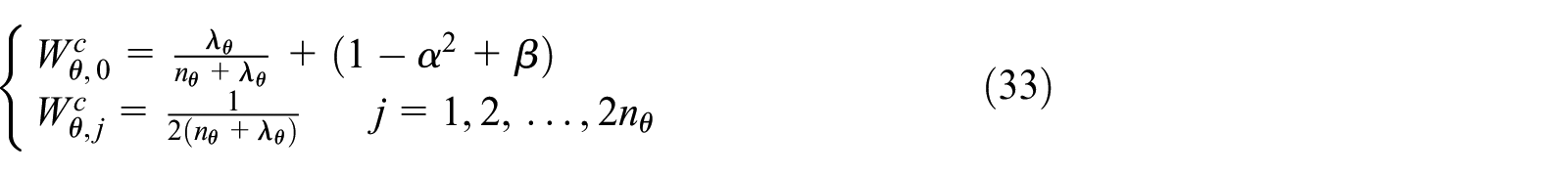
where n_θ is the dimension of the parameter vector and λ_θ is the coefficient of the sampling point equation (21).

7. Parameter correction

We use the estimated states and measured observations to correct the parameter vector. The parameter correction includes the correction of the parameter vector and the covariance of parameter error.

First, the observation equation given by equation (14) performs a nonlinear transformation on a set of Sigma sampling point of the parameter vector

γ_{θ j, k + 1} = h ({\hat{x}}_{k + 1}, u_{k + 1}, χ_{θ j, k + 1})

(34)

The estimated value of the observation vector and its covariance are obtained by weighting

{\hat{y}}_{θ, k + 1} = \sum_{j = 0}^{2 n_{x}} W_{θ, j}^{m} γ_{θ j, k + 1}

(35)

P_{y, k + 1}^{θ} = \sum_{j = 0}^{2 n_{θ}} W_{θ, j}^{c} (γ_{θ j, k + 1} - {\hat{y}}_{θ, k + 1}) {(γ_{θ j, k + 1} - {\hat{y}}_{θ, k + 1})}^{T} + R_{θ}

(36)

where R_θ is the covariance matrix of the observation noise.

Then, the cross-covariance between the parameter vector and the observation vector, and the Kalman gain matrix of the parameter vector are calculated

P_{θ y, k + 1} = \sum_{j = 0}^{2 n_{θ}} W_{θ, j}^{c} (χ_{θ j, k + 1} - {\hat{θ}}_{k + 1}^{-}) {(γ_{θ j, k + 1} - {\hat{y}}_{θ, k + 1})}^{T}

(37)

K_{θ, k + 1} = P_{θ y, k + 1} {(P_{y, k + 1}^{θ})}^{- 1}

(38)

Finally, the posterior estimation of the parameter vector and the covariance of the state error are calculated and updated, respectively

{\hat{θ}}_{k + 1} = {\hat{θ}}_{k + 1}^{-} + K_{θ, k + 1} (y_{k + 1} - {\hat{y}}_{θ, k + 1})

(39)

P_{θ, k + 1} = P_{θ, k + 1}^{-} - K_{θ, k + 1} P_{y, k + 1}^{θ} K_{θ, k + 1}^{T}

(40)

DUKF framework

In equation (14), the state vector includes longitudinal velocity, lateral velocity, yaw rate, roll angle, roll velocity, yaw moment, longitudinal acceleration, and lateral acceleration

x = {[\begin{matrix} u & v & r & ϕ & \overset{\cdot}{ϕ} & M_{z} & a_{x} & a_{y} \end{matrix}]}^{T}

(41)

The state equation of the Eulerian discrete velocity and the state transition matrix are obtained, respectively, as

{[\begin{matrix} u \\ v \\ r \\ ϕ \\ \overset{\cdot}{ϕ} \\ M_{z} \\ a_{x} \\ a_{y} \end{matrix}]}_{k + 1} = {[\begin{matrix} \overset{\cdot}{u} \\ \overset{\cdot}{v} \\ \overset{\cdot}{r} \\ \overset{\cdot}{ϕ} \\ \overset{\cdot\cdot}{ϕ} \\ 0 \\ 0 \\ 0 \end{matrix}]}_{k} \times Δ T + {[\begin{matrix} u \\ v \\ r \\ ϕ \\ \overset{\cdot}{ϕ} \\ M_{z} \\ a_{x} \\ a_{y} \end{matrix}]}_{k}

(42)

Φ_{x} = I + J_{x} \cdot Δ T

(43)

where I is the unit matrix and ΔT is the sample time, which is set to 0.01 s.

In this article, we use the vehicle mass, yaw moment of inertia, and position of the mass center as the parameter vector (as shown in equation (44)). Since the position of the mass center is located between the second axle and the third axle for the four-axle vehicle, it is represented by the distance from the mass center to the second axle L₂

θ = {[\begin{matrix} m & I_{zz} & L_{2} \end{matrix}]}^{T}

(44)

According to the structural feature of the four-axle distributed electric vehicle, the steering angle of the first two axles, the motor torque, and angular rate of the eight electric wheels are selected as the input vector of the DUKF estimator

u (t) = {[\begin{matrix} \begin{matrix} δ_{1 l} & δ_{1 r} & δ_{2 l} & δ_{2 r} \end{matrix} & ω_{i} & T_{i} \end{matrix}]}^{T}

(45)

Besides, we take the lateral acceleration and the yaw rate as the observation vectors in DUKF

y = {[\begin{matrix} a_{y} & r \end{matrix}]}^{T}

(46)

After discretization of the vehicle dynamics model and the selection of the state vector and the parameter vector, the joint estimator based on DUKF can be implemented recursively, as shown in Figure 2. In addition, the number of Sigma sampling points depends on the dimension of the state vector and the parameter vector. In light of the symmetric point sampling, the numbers of Sigma points of the state vector and the parameter vector are 17 and 7, respectively.

In the vehicle joint estimator as shown in Figure 3, the vehicle dynamics model provides control variables including steering angle of the first two axles, angular rate, and motor torque of each electric wheel to the tire dynamics model, and then the tire model outputs the longitudinal force and lateral force of tire to the DUKF estimator. The vehicle dynamics model also provides steering angle of the first two axles and observations such as yaw rate and lateral acceleration to the DUKF estimator. In addition, the estimated longitudinal velocity, lateral velocity, and yaw rate from the DUKF estimator are fed back to the tire model.

Figure 3.

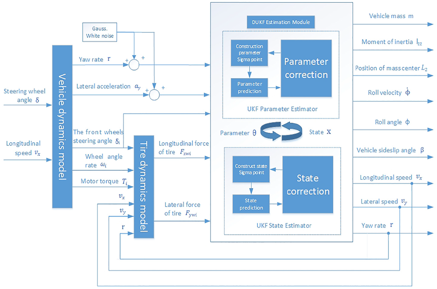
Diagram of DUKF joint estimator.

Simulation and analysis

The DLC condition and sinusoidal input of steering wheel angle condition are used to verify the DUKF estimator by Simulink/TruckSim simulation. However, the four-axle vehicle model in TruckSim needs to be modified as the distributed electric vehicle, and the modeling method is available in Xiong et al.²⁴ The vehicle speed is assumed to be 60 km/h, and the road adhesion coefficient is 0.9. Then, vehicle parameters are set according to Table 1 except the three parameters to be estimated.

Table 1.

Parameter settings of the TruckSim vehicle.

Unit	Parameter	Value
m (kg)	Vehicle mass	12,200
L ₁ (m)	The distance from the first axis to the second axle	1.3
L ₂ (m)	The distance from the center of mass to the second axle	0.5
L ₃ (m)	The distance between centroid and the third axle	0.85
L ₄ (m)	The distance from the third axle to the fourth axle	1.35
m_s (kg)	Sprung mass	10,000
B (m)	Wheel track	1.863
h (m)	Height of the mass center	1.2
I_zz	Yaw moment of inertia	60,000
I_xx	Roll moment of inertia	7000

DLC condition

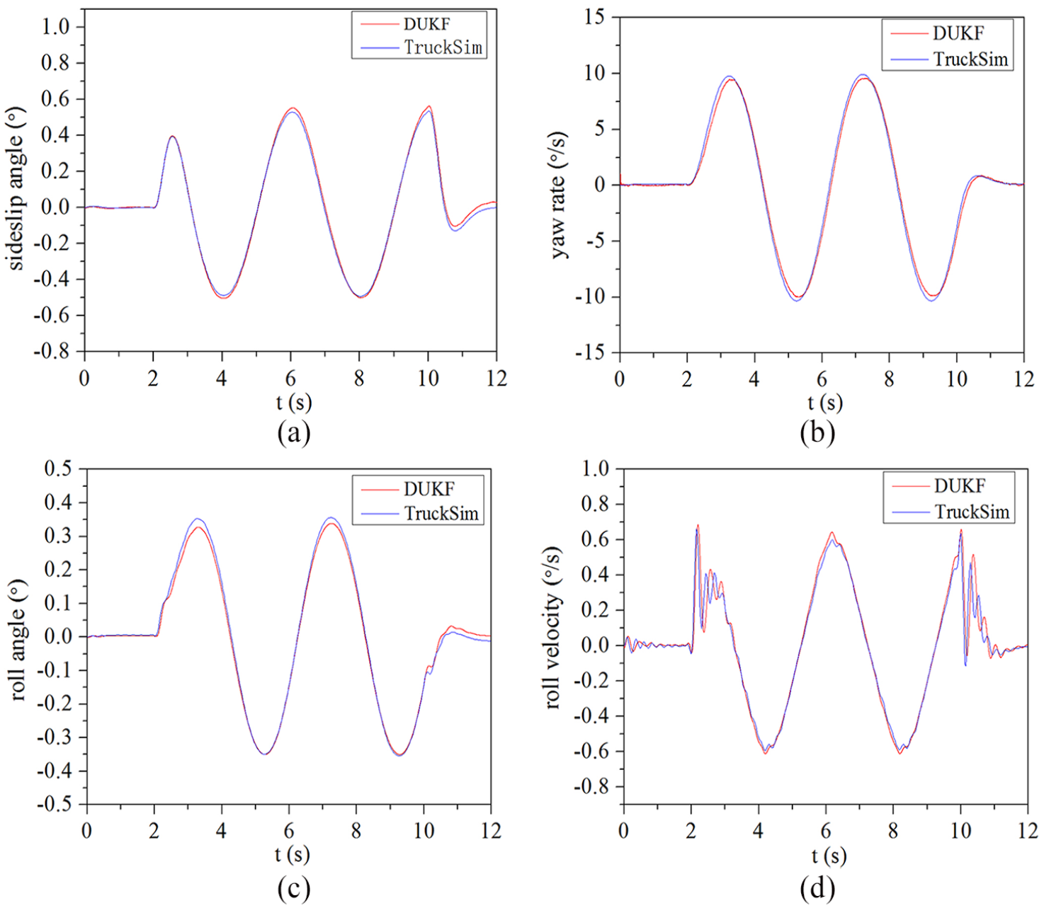
As the input of the DUKF estimator, we set vehicle velocity to 60 km/h and the steering wheel angle according to Figure 4. First, we compare the estimated values of vehicle state with the output of vehicle model. The results of state estimation are shown in Figure 5. It can be seen that the estimated results of the vehicle state are consistent with the overall trends in the outputs from TruckSim.

Figure 4.

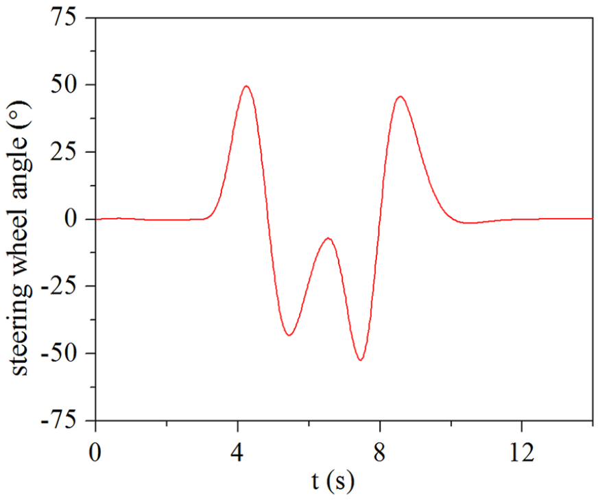
Steering wheel angle in DLC.

Figure 5.

DUKF results of state estimation in DLC: (a) vehicle sideslip angle, (b) yaw rate, (c) roll angle, and (d) roll velocity.

According to the estimation error shown in Table 2, the maximum error is very small and the maximum relative error is less than 5%. This estimated error is within a reasonable range, so the DUKF estimator of state has a high accuracy.

Table 2.

DUKF error of state estimation in DLC.

	Vehicle sideslip angle	Yaw rate	Roll angle	Roll velocity
Maximum error	0.023 (°)	0.1 (°/s)	0.009 (°)	0.01 (°/s)
Maximum relative error	4.4%	1.8%	4.9%	2.5%

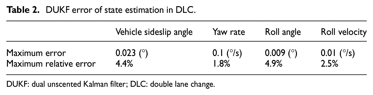
DUKF: dual unscented Kalman filter; DLC: double lane change.

For the estimator of parameter, we set the initial value of vehicle mass, yaw moment of inertia, and distance from the second axle to the mass center to 10,000 kg, 50,000 kg m², and 0.3 m, respectively. The estimated values of vehicle parameter are compared with its nominal value in Table 1, and estimated results are shown in Figure 6.

Figure 6.

DUKF results of parameter estimation in DLC: (a) vehicle mass, (b) yaw moment of inertia, and (c) distance from second axle to mass center.

It can be seen from the above estimation results that three parameters accelerate the convergence when vehicle starts to turn at time 3 s, and they are close to the nominal term in a short time. Although the distance from the second axle to the mass center would fluctuate in a small range during DLC, the overall trend is convergence and eventually stabilized at time 10 s. Since the observations including vehicle’s yaw rate and lateral acceleration have a strong correction effect on the estimated parameters, they can quickly converge to the nominal value after one process of DLC.

Sinusoidal steering condition

We set the vehicle velocity to 60 km/h and sinusoidal input of steering wheel angle as shown in Figure 7. The vehicle parameters are set as in Table 1. Using the DUKF estimator, the vehicle state and output parameters are achieved under sinusoidal steering condition. The results of state estimation are shown in Figure 8.

Figure 7.

Sinusoidal input of steering wheel angle.

Figure 8.

DUKF results of state estimation under sinusoidal steering condition: (a) vehicle sideslip angle, (b) yaw rate, (c) roll angle, and (d) roll velocity.

It can be seen that the estimated state including longitudinal velocity, sideslip angle, yaw rate, roll angle, and roll velocity have a good consistency with the corresponding output of vehicle model, and the estimation errors are shown in Table 3. The indexes of estimation accuracy indicate both the maximum error and the maximum relative error are less than 5%. Although the error is increased compared with the DLC condition, it is still within a reasonable and small range. Therefore, the introduction of parameter correction makes the estimation of state more accurate by better compensation for the mismatch of model parameters. However, the estimation error of DUKF cannot converge to 0 since it is caused by unknown random signal noise, or unmodeled dynamics system cannot be eliminated completely.

Table 3.

DUKF error of state estimation under sinusoidal steering condition.

	Vehicle sideslip angle	Yaw rate	Roll angle	Roll velocity
Maximum error	0.027 (°)	0.2 (°/s)	0.014 (°)	0.031 (°/s)
Maximum relative error	4.5%	2%	3.9%	4.7%

DUKF: dual unscented Kalman filter.

Three vehicle parameters estimated by DUKF are compared with the nominal values, as shown in Figure 9. After turning the steering wheel at time 2 s, the vehicle mass converges to nominal terms quickly. At the same time, the distance from the second axle to the mass center approaches the nominal value and fluctuates within a small range with the varying steering wheel angle. In addition, the yaw moment of inertia is close to its nominal value gradually, and finally steady at time 10 s. During the sinusoidal steering situation, the estimation of three parameters is achieved because the observations such as yaw rate and lateral acceleration would have a strong correction to the estimated parameters.

Figure 9.

DUKF results of parameter estimation under sinusoidal steering condition: (a) vehicle mass, (b) yaw moment of inertia, and (c) distance from second axle to mass center.

From the estimation results under DLC condition and sinusoidal steering condition, we can see that the DUKF estimator has a good effect on the estimation of vehicle state and parameters. By real-time estimation of vehicle parameters, the problem of unknown parameter or its dynamic change can be solved. Furthermore, the accuracy of state estimation can be improved with compensation of parameter error.

Conclusion

Considering some parameters of heavy vehicle such as vehicle mass, yaw moment of inertia, and position of mass center are hard to measure or change during driving, a parameter estimator is introduced on the basis of the state estimator. In this article, we proposed a DUKF estimator for multi-axle distributed electric vehicle. The simulation results show that the proposed estimator has a good estimation accuracy for vehicle state without the influence of parameter errors. At the same time, the key parameters could converge to the nominal terms quickly by parameter correction of joint estimation. In future, an adaptive DUKF algorithm will be applied, and more real test of heavy vehicle under different road adhesion is needed.

Footnotes

Declaration of conflicting interests

The author(s) declared no potential conflicts of interest with respect to the research, authorship, and/or publication of this article.

Funding

The author(s) disclosed receipt of the following financial support for the research, authorship, and/or publication of this article: This work was financially supported in part by the National Natural Science Foundation of the People’s Republic of China (grant number: 51675390). The authors would like to thank the reviewers and the Associate Editor for their helpful and detailed comments, which have helped to improve the presentation of this article.

ORCID iD

Xiaofei Pei

Author biographies

Xiaofei Pei received B.E. degree from Wuhan University of Technology, China, in 2007, and received Ph.D degree from Beijing Institute of Technology, China, in 2013. He is now an associate professor in Wuhan University of Technology from 2016. His research field are vehicle dynamic and control, vehicle safety, ADAS, etc.

Zhenfu Chen received B.S. degree in vehicle engineering, from Wuhan University of Technology, China, in 1984, and received Ph.D degree from TU Braunschweig, Germany, in 1991. He is now a visiting professor in Wuhan University of Technology from 2012. His research interest includes vehicle brake system, vehicle longitudinal control and active safety.

Bo Yang received B.E. degree from Tsinghua University, China, in 1997, and received Ph.D degree in M.E. from Huazhong University of Science and Technology, China, in 2004. He is now an associate professor in Wuhan University of Technology from 2006. His research field are heavy vehicle design, vehicle dynamics, etc.

Duanfeng Chu received B.E. and Ph.D degree from Wuhan University of Technology in 2005 and 2010, respectively. He is now an associate professor in Wuhan University of Technology from 2012. His research field are ITS, autonomous vehicle, etc.

References

Guo

Chen

Zhao

, et al. State and parameter estimation for running vehicle: recent developments and perspective. Control Theory Appl 2013; 30(6): 661–672.

Gao

. Review of vehicle state estimation problem under driving situation. J Mech Eng 2009; 45(5): 20–33.

Chen

Hsieh

. Sideslip angle estimation using extended Kalman filter. Vehicle Syst Dyn 2008; 46: 353–364.

Gao

Chen

, et al. Fusion estimation of vehicle sideslip angle. Automot Eng 2013; 36(8): 716–722.

Sun

Yan

, et al. A hybrid algorithm combining EKF and RLS in synchronous estimation of road grade and vehicle′ mass for a hybrid electric bus. Mech Syst Signal Pr 2016; 68: 416–430.

Kang

Kim

, et al. Adaptive side slip angle observer using simple combined vehicle dynamics. In: Proceedings of the 16th international IEEE conference on intelligent transportation systems, The Hague, 6–9 October 2013, pp. 85–90. New York: IEEE.

Zhang

Wang

. State estimation for a four-wheel independent drive electric ground vehicle. In: Proceedings of the 34th Chinese control conference, Hangzhou, China, 28–30 July 2015, pp. 8073–8078. New York: IEEE.

Wang

Cheng

Victorino

, et al. Nonlinear observers of tire forces and sideslip angle estimation applied to road safety: simulation and experimental validation. In: Proceedings of the 2012 IEEE intelligent transportation systems conference, Anchorage, AK, 16–19 September 2012.

Ungoren

Peng

Tseng

. A study on lateral speed estimation methods. Int J Veh Auton Syst 2002; 2(1–2): 126–144.

10.

Katriniok

Abel

. Adaptive EKF-based vehicle state estimation with online assessment of local observability. IEEE T Contr Syst T 2016; 24(4): 1368–1381.

11.

Sarkka

. On unscented Kalman filtering for state estimation of continuous-time nonlinear systems. IEEE T Automat Contr 2007; 52(9): 1631–1641.

12.

Jiang

Corrêa

Ali

. Real-time estimation of vehicle’s lateral dynamics at inclined road employing extended Kalman filter. In: Proceedings of the IEEE 11th conference on application, Hefei, China, 5–7 June 2016, pp. 2360–2365. New York: IEEE.

13.

Sebsadji

Glaser

Mammar

, et al. Road slope and vehicle dynamics estimation. In: Proceedings of American control conference, Seattle, WA, 11–13 June 2008, pp. 4603–4608. New York: IEEE.

14.

Dakhlallah

Glaser

Mammar

, et al. Tire-road forces estimation using extended Kalman filter and sideslip angle evaluation. In: Proceedings of American control conference, Seattle, WA, 11–13 June 2008, pp. 4597–4602. New York: IEEE.

15.

Best

Gordon

Dixon

. An extended adaptive Kalman filter for real-time state estimation of vehicle handling dynamics. Vehicle Syst Dyn 2000; 34(1): 57–75.

16.

Antonov

Fehn

Kugi

. Unscented Kalman filter for vehicle state estimation. Vehicle Syst Dyn 2011; 49(9): 1497–1520.

17.

Doumiati

Victorino

Charara

, et al. On board real-time estimation of vehicle lateral tire-road forces and sideslip angle. IEEE/ASME T Mech 2011; 16(4): 601–614.

18.

Geng

Mostefai

Denai

, et al. Direct yaw-moment control of an in-wheel-motored electric vehicle based on body slip angle fuzzy observer. IEEE T Ind Electron 2009; 56(5): 1411–1419.

19.

Chen

Zong

. Based on the unscented Kalman filter to estimate the state of four-wheel-independent electric vehicle with X-by-Wire. SAE Int J Commer Veh 2015; 8(2): 316–322.

20.

Nam

Fujimoto

Hori

. Lateral stability control of in-wheel-motor-driven electric vehicles based on sideslip angle estimation using lateral tire force sensors. IEEE T Veh Technol 2012; 61(5): 1972–1985.

21.

Wenzel

Burnham

Blundell

, et al. Dual extended Kalman filter for vehicle state and parameter estimation. Vehicle Syst Dyn 2006; 44(2): 153–171.

22.

Xie

Wei

, et al. Vehicle state and road friction coefficient estimation based on double cubature Kalman filter. Sci Sin Tech 2015; 45(4): 403–414.

23.

Oda

Yoshida

Shimizu

. Marketing strategy of Eliica, the 370km/h max speed electric vehicle. In: Proceedings of the 21th international battery, hybrid and fuel cell electric vehicle symposium & exposition, Monte Carlo, 2–6 April 2005.

24.

Xiong

Chen

Feng

. Modeling of distributed drive electric vehicle based on co-simulation of Carsim/Simulink. J Syst Simul 2014; 26(5): 1143–1155.

Estimation of states and parameters of multi-axle distributed electric vehicle based on dual unscented Kalman filter

Abstract

Keywords

Introduction

Modeling of multi-axle distributed electric vehicle

Modeling overview

Vehicle dynamics

Tire dynamics

DUKF algorithm

Algorithm overview

DUKF framework

Simulation and analysis

DLC condition

Sinusoidal steering condition

Conclusion

Footnotes

Declaration of conflicting interests

Funding

ORCID iD

Author biographies

References