Sage Journals: Discover world-class research

Abstract

Sexually motivated crime (SMC) has an immense and ongoing impact on victims, victim-survivors, their families, and the broader society, such that countless resources and forensic techniques have been deployed in pursuit of prosecuting perpetrators. For law enforcement investigating sexual crimes, linkage between incidents is an important tool to identifying serial offenders as well as victims that are unattributed or part of unsolved cold cases. Serial sex offending is well reported making it likely that operating or dormant sexually motivated offenders that have gone undetected and are still at large. To assist in solving these challenges a technique that can link victims of these crimes beyond victimology and modus operandi is needed. This research develops Face Similarity Linkage as a forensic tool to identify minute variations in facial anthropometry to detect similarities between victims of SMC as intelligence for further investigation. Several tests, detecting interobserver error and camera angle variation were used to determine which facial landmark measurements were most useful in differentiating three random, unrelated faces from an available dataset. Our study revealed 55 ratios of various point-to-point measurements that show promise for future studies using this technique. While there was some variation between readers, it was approximately 5% or less and could be improved with additional training of readers.

Keywords

sexually motivated crime facial biometrics cold case forensic anthropometry face similarity linkage

Introduction

It is not uncommon for any member of society to have a particular preference of the sexual partners to whom they are attracted (Huston and Levinger, 1978; Mark and Herbenick, 2014). This is often overt, by way of a particular hair or eye colour, stature, or racial ancestry to which one is physically attracted (Cornwell et al., 2006; Langlois et al., 2000). It is equally possible that much less noticeable characteristics attract sexual partners to one another - perhaps a face shape, nose, mouth or lip characteristics, or general facial geometry (Penton-Voak et al., 2001; Penton-Voak and Perrett, 2000; Perrett et al., 1998). These factors that make an individual sexually “attractive” to someone may lie within a subconscious decision process in determining pairings, just as other mate-attracting features are seen in the wild (Mark and Herbenick, 2014)¹. While the motivations for sexual attraction may seemingly belong well outside of policing matters, new forensic biometric tools may allow for better insight into criminals’ selection of sexual assault and homicide victims.

While there is scant peer reviewed evidence to the suggestion, some sexually motivated perpetrators may be subjected to an overt or subconscious decision process driven by their victims’ physical characteristics. Studies have shown that features of the victimology such as age, sex, class and elements of physical appearance do influence an offender’s choice of victim (Hazelwood and Warren, 2003; Labuschagne, 2014; Winter et al., 2013). One such example made record of fantasies about body shape, length and colour of hair and breast size of their victim (Hazelwood and Warren, 2003). Glen Edward Rogers was named “The Red Head Killer” because of his predilection for auburn-haired victims (Linedecker, 1997). It is also common and widely reported that many serial killers seek out victims with similar physical characteristics to an opposite-sex parent or close family member who inflicted childhood trauma (LaBrode, 2007; Schlesinger, 1998). This has been noted in criminal cases wherein offenders will seek out those who represent a previous person who has wronged or hurt them (e.g., Joseph DeAngelo). Like Rogers, Theodore Bundy has been similarly reported as having a proclivity for a particular hair colour (brunette victims), notably with their hair parted in the middle, thought to have been triggered by the breakup with his first girlfriend, who had a similar appearance (Rule, 2018). While these similarities may appear clear to the casual observer, and make for useful layperson comparisons in the media, for them to be useful in investigations an element of scientific rigor is required.

As well as increasing the opportunity to understand a criminal profile of sexually motivated perpetrators, the ability to link multiple victims of a single offender to each other by their similarities would prove a helpful intelligence tool for investigators. Many convicted serial killers have lists of victims, formally attributed through trial proceedings and leading to a conviction. In many cases, several additional victims that are not legally associated remain ‘unresolved’. For example, murderer Samuel Little confessed to many more victims than he was formally charged with. Often these additional victims have been linked through victim typology and the killer’s modus operandi (MO), while in others, they get attributed through confessions or self-reporting by the accused. If a homicide accused has been tried and convicted for a sentence of either life imprisonment or death, it is common for no further legal proceedings to be carried. It does not benefit the state or jurisdiction to mount further costly trial proceedings if an offender has already received a maximum sentence. As such, many homicide victims only get linked informally to an offender, lacking a formal conviction. Forensic challenges can also prevent individual victim cases from going to trial, particularly if forensic evidence is insufficient. Further hurdles include situations where sexual assault cases go unreported, are reported well after the offence, or those whereby a complaint is withdrawn for fear of revictimization (B.Hall & B.Chapman, 2026). In homicides where victim remains are undiscovered, even more difficulty is faced. A new method that could help link victims-to-victims and, by inference, victims-to-killers, may provide investigative leads for resolving some of these cases.

There are challenges in associating an authentic and comprehensive list of victims to serial offenders that limits the proper attribution of victims, particularly without DNA linking them. In the case of serial homicide, many serial killers falsely claim extra victims to inflate their victim tallies for increased attention and notoriety (Kelly & Lynes, n.d). Secondly, in the years spanning 1965 to 2020 there were over 330,000 unsolved homicide cases (Hargrove, 2019) in the United States alone, with approximately 1% of these homicides thought to be linked to serial killers (L.G. Johns, M.E. O’Toole, T.G. Keel, D.T. Resch, S.F. Malkiewicz, M. Safarik, J.J. McNamara, A.A. Showalter, K.R. Mellecker, 2008). If that proportion was applied to those unsolved, then there may be as many as 3300 unsolved homicides linked to either an already convicted or unidentified serial killer in the United States. Serial sexual assault is even more pronounced with one study reporting that 63% of rapists declared repeated offences, averaging 5.8 rapes each (Lisak and Miller, 2002). The question of how to identify a sexual assault or homicide victim from other non-serial crimes emerges. For the specific subset of serial offenders motivated by sexual intent, subtle characteristics of a victim’s facial geometry could provide valuable intelligence to law enforcement.

The use of facial biometric tools is a growing capability in both consumer information technology devices and government and security applications (Jain et al., 2004). The most straightforward way of categorising facial biometrics is by dividing approaches into one-to-one or one-to-many algorithms (Flores et al., 2019). A one-to-one application of facial biometrics is where a user’s facial geometry is collected and stored on a device or dataset. When users wish to authenticate to a system, such as a mobile phone to unlock it, they present their face to a camera or detector that verifies multiple landmarks against the stored dataset. Once a match is made, the user is authenticated, and access is granted. This process happens in a very short time, appearing almost instantaneous in modern devices like smartphones (Galterio et al., 2018). The one-to-many use of facial biometrics is when many people’s facial geometries are stored on a database that is searched to identify a single user or person. A typical scenario that demonstrates this is government databasing of driver’s licence or passport photos. If an unknown individual needs to be identified, such as from closed circuit television (CCTV) footage, their facial geometry can be searched against the database, and identification or a shortlist is generated (Facial Identification Working Group, 2012; Martos et al., 2018).

To date, facial biometrics have only been used for the identification or verification of a single person. The first manuscript within crime research using facial geometry to compare different individuals was with a method named Face Similarity Linkage (FSL) by Hackett et al. (Hackett et al., 2020). This provided a proof of concept for the linkage of SMC victim facial characteristics, in that case, those associated with the victims of Theodore Bundy. Hackett et al. (Hackett et al., 2020) outlined a rudimentary approach and acknowledged the method’s many limitations.

This research builds on the FSL technique in three ways. The first aim was to evaluate which facial landmarks are more powerful in differentiating one random individual from another. This will help establish a more a robust understanding of the most suitable facial landmarks to drive this technique forward. Secondly, one of the noted limitations of using victim images derived from online and personal photo collections, is that the angle at which the image is taken is often off the full-frontal plane. This is dissimilar to the strict parameters of passport-style photos normally used in facial biometrics, so this work aimed to identify reliable landmarks in offset images. Finally, in addition to improving these facial geometry aspects of the FSL, this research also aimed to adapt the hand-measured methodology used in Hackett et al. (Hackett et al., 2020) by a single reader to a multiple replicate, in-silico technique that is more amenable to machine learning automation in future iterations.

Method

Images and data acquisition

Three donor faces (identified as B28, B32 and B34 by the image source) were chosen randomly from the Yale Faces Database (Belongie et al., 2001). This database was chosen because it contained individual faces with multiple grayscale images taken at varying angles to the face (Figure 1). These angles are typically found in the type of images of victims provided to law enforcement from family members and friends or sourced from social media.

Figure 1.

The nine images of one donor from the Yale Faces Database B (21) used in this study. Two-digit numbers correspond with the filename conventions used by publishers of the images with 00 reflecting a full-frontal photograph without any camera angle skew. Deviations from that angle are described as being either neutral, high, or low in the transverse plane (TP), (No TP, High TP, and Low TP, respectively) or with none, small or large offset of the camera in the sagittal plane (SP), (No SP, Small SP and Large SP, respectively).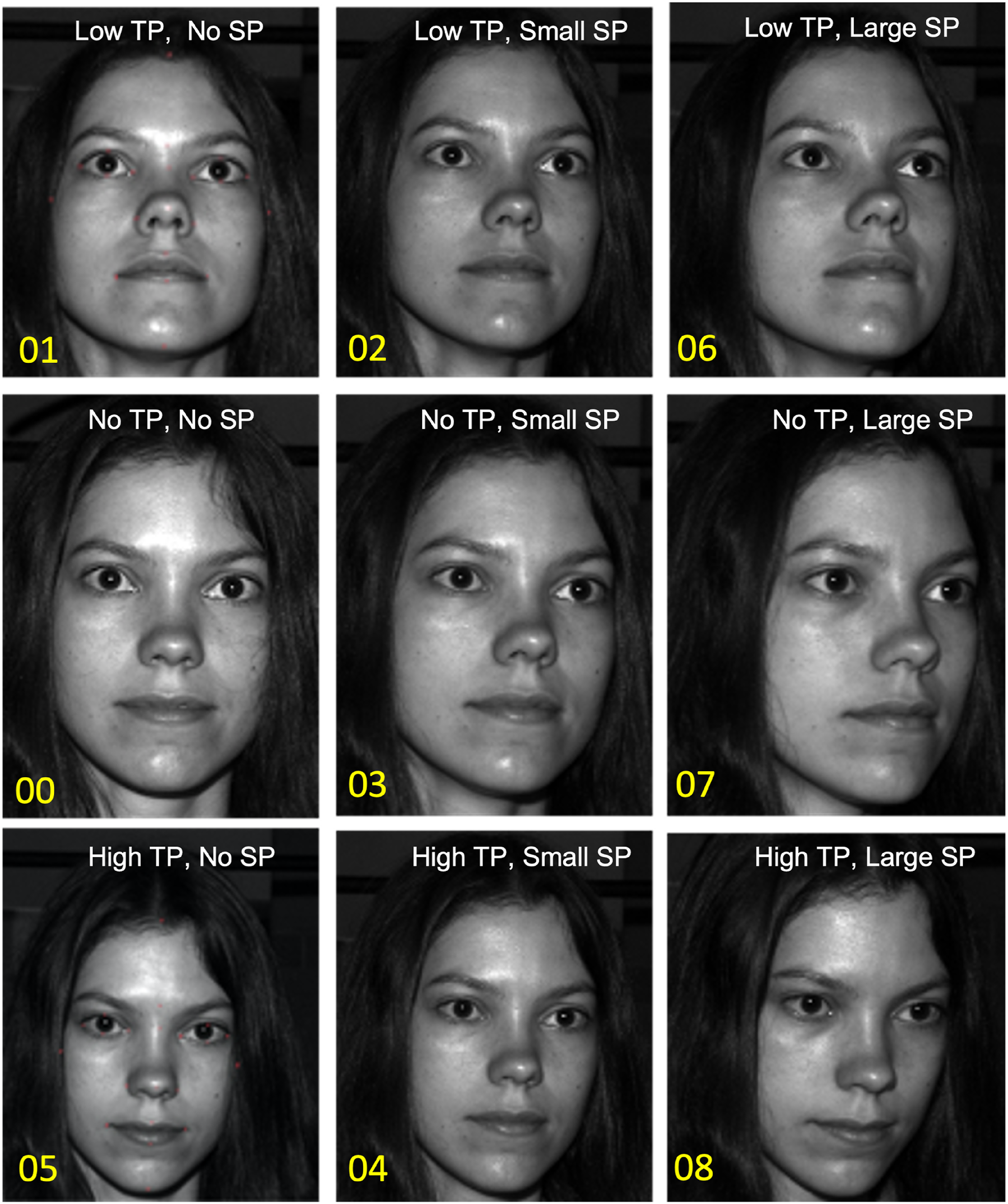

Anatomical descriptors for planes were used in describing the camera angle. The transverse plane (TP) was defined as being either neutral (No TP), low (Low TP) or high (High TP) with respect to the “camera”. The sagittal plane was defined as being either straight on (No SP), offset at a small angle (Small SP) or offset by a large angle (Large SP).

Twenty-one landmarks were annotated on the images using a tablet and stylus (Apple® iPad™ and Pencil™ within the native Photos™ application) in a contrasting colour to the grayscale so that they could be easily identified in later parts of the analysis. These landmarks were chosen as they included those used in Hackett et al. (Hackett et al., 2020), except for superciliare centralis (centre of eyebrow, highest point), ciliare medialis (most medial and inferior corner of eyebrow), and ciliare lateralis (most lateral extent of eyebrow). These three exclusions were made because they all related to the eyebrow, which is often a cosmetically modified characteristic. Annotated images were then imported into Adobe® Photoshop™ (Adobe Inc., 2004) and measurements were taken from 19 point-to-point (PtP) distances (Figure 2) using the Photoshop ruler tool to generate a table of pixel counts. Measurements were collated into Microsoft® Excel™ and arrayed into a table allowing for each measurement to be divided by every other measurement to generate a list of ratios, that is;

\frac{M e a s u r e m e n t 1}{M e a s u r e m e n t 2}, \frac{M e a s u r e m e n t 1}{M e a s u r e m e n t 3}, \frac{M e a s u r e m e n t 1}{M e a s u r e m e n t 4} etc .

Figure 2.

A stylised diagram to illustrate the 21-point landmarks (red circles) and the 19 pixel count measurements. Nomenclature was taken from Lee et al. (23) and is abbreviated as: TR = Trichion, GN = Gnathion, G = Glabella, N = Nasion, PN = Pronasale, LS = Labiale superius, LI = Labiale inferius, EX = Exocanthion*, EN = Endocanthion, ZY = Zygion*, AL = Alare*, CH = Chellion*, PS = Palpebral superius*, PI = Palpebrale inferius* (NB: * denotes that these measurements were taken from the left (l) and right (r) side of the person in the image).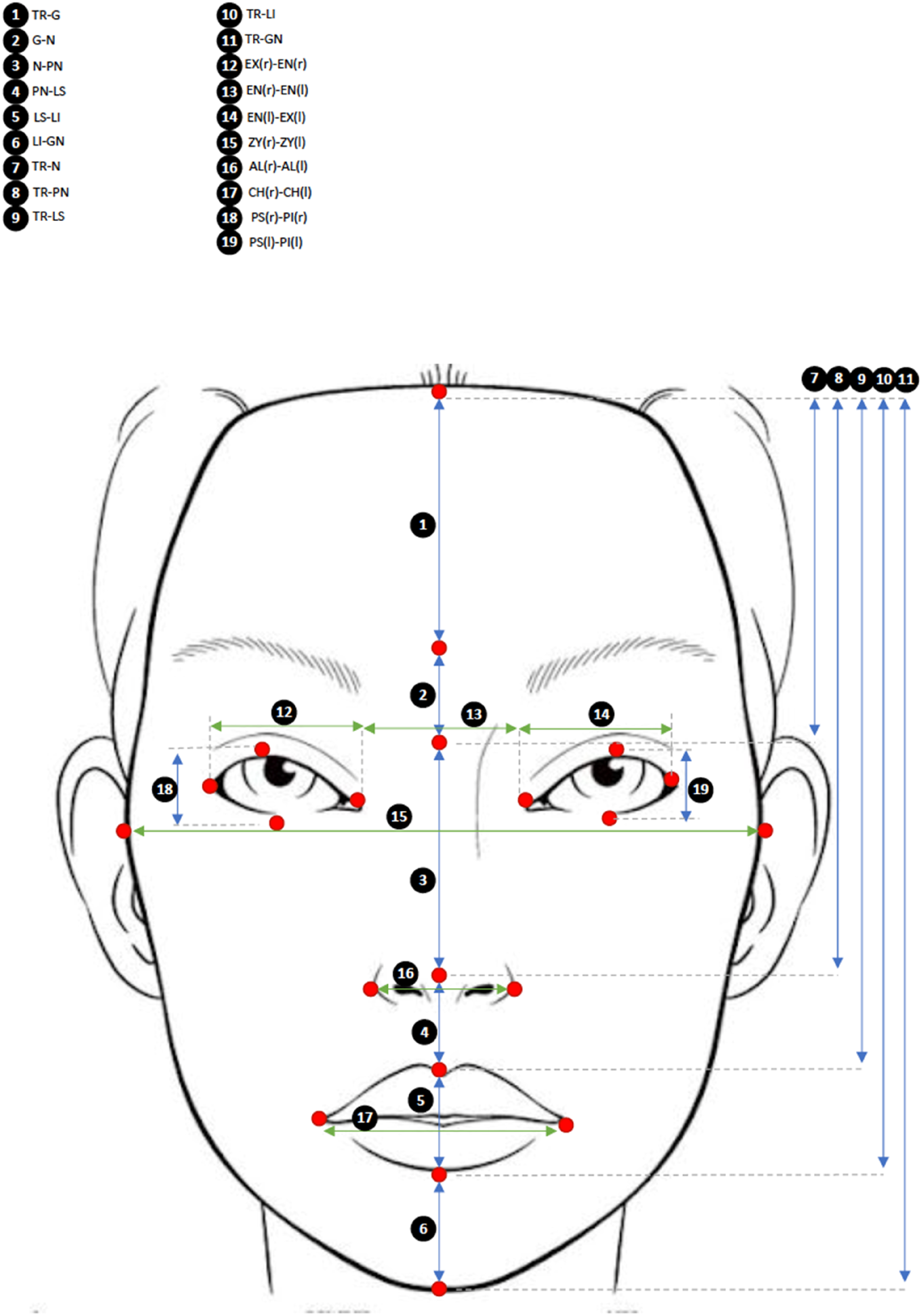

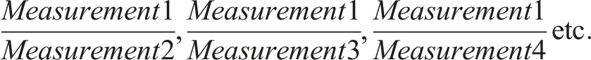
Ratios were used to remove the variability in absolute pixel counts owing to the differences in camera settings and a lack of scaled rulers in these images and any images that law enforcement will have access to. In real casework, there are unlikely to be any scaled images available, so the generation of ratios allows for the removal of absolute lengths and provides utility for real world scenarios. To achieve this, each pixel measurement had a ratio of it to another measurement calculated. For example, a ratio was calculated between lip width and eye width, lip width and forehead depth, and so on. 342 ratios were generated for each image, totalling 3078 ratios for each of the three faces. To ensure that the technique was not operator dependent, three readers undertook independent measurements using the same method. Reader 1 was the lead author of the study and Readers 2 and 3 were junior interns provided with simple instructions on the collection of the measurements along with the diagram in Figure 2, as well as the Hackett et al. (Hackett et al., 2020) paper describing the landmarks. This provided 9234 datapoints per reader in total for the study.

Interobserver error

For each of the three faces, B28, B32 and B34, at each of the nine camera angles, three reader results were compared using technical error of measurement (TEM) calculated between each reader, i.e., r1 to r2, r1 to r3, r2 to r3. This enabled the differentiation of each camera angle to detect angles that were susceptible to user variation. Single factor analysis of variance (ANOVA) tests were used to identify statistical differences both within and between readers.

Individual differentiation

Data for a single reader were analysed by comparing PtP measurement ratios for variation between the three participant faces for all camera angles.

Shapiro-Wilk and D’Agostino tests for normality were conducted on each set of repeated measurements across the nine camera angles and three faces (27 data points). Not all data were normally distributed, therefore statistical tests dependent on normality were not considered. The Coefficient of Variance (CV) was calculated and dot-plots for each set of ratios generated using GraphPad Prism v9.3.1 for Mac (GraphPad Software, San Diego, California USA, https://www.graphpad.com/). CVs were then compared to determine the PtP measurement ratios with the greatest variability in this data set.

Identifying ratios with a high and low susceptibility to changes in camera angle

For each of the three readers, across all three donor faces, a CV was calculated between the same measurements at each of the nine camera points of view. An arbitrary threshold was set (>20%, in red, Supplemental Data 1a, b and c) to flag any ratios that had a high CV across the nine different angles, indicating measurements that could be deemed as heavily influenced by camera angle. Conversely, angles with a low CV (again, arbitrarily defined, this time as <5%, in green, Supplemental Data 1a, b and c) were also flagged, as these ratios indicated that the associated measurements were unvaried, regardless of the camera angle. An example of the arrays generated is shown in Figure 3. Any of the 18 point-to-point CVs with greater than 4 data points (out of 18 total) either flagged as high or low were coloured with red or green, respectively. This way, visually, each of the PtP measurements could be seen as “good” or “bad” in terms of its ability to withstand variation in camera angle. Uncoloured data were all of those with CVs falling between 5% and 20% and were considered as “neutral”.

Figure 3.

One selection (Reader 3) of arrayed CV data coloured to show high and low variation brought about by camera angle. Left to right, arrays coincide with B28, B32 and B34.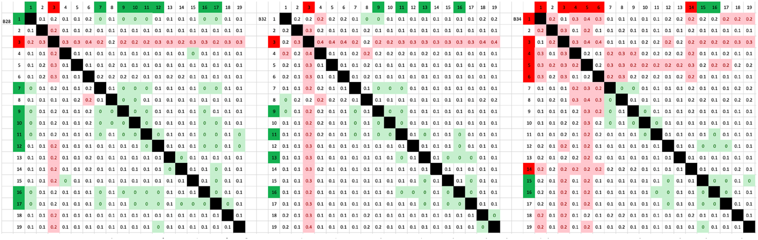

Proof of concept test

A final principal component analysis (PCA) (like that used in Hackett et al. (Hackett et al., 2020)) was conducted of frontal images of the three faces using 55 PtP ratios determined to be optimal from the previous tests. ClustVis (Metsalu and Vilo, 2015) PCA visualiser was used to visualise PCA plots and heatmap data.

Results and discussion

Interobserver error

All 19 PtP measurements were compared across the three faces, their subsequent nine camera angles and between three readers to ascertain whether any measurements carried greater user variation. The summary of these data is shown in Table 1.

Table 1.

Technical Error of Measurement proportions across three readers (r1, r2 and r3) for the nine camera angles of 3 faces (B28, B32 and B34).

	TEM (%)
	r1_r2	r1_r3	r2_r3	Mean	SD
No TP, No SP	5.8	2.5	3.3	3.9	1.7	B28
Low TP, No SP	1.7	0.6	1.1	1.1	0.6
Low TP, small SP	7.0	1.3	8.3	5.5	3.7
No TP, small SP	11.2	1.5	9.6	7.5	5.2
High TP, small SP	12.6	3.6	8.9	8.4	4.5
High TP, No SP	6.7	0.8	7.5	5.0	3.7
Low TP, large SP	4.7	5.1	0.5	3.4	2.6
No TP, large SP	4.5	0.9	3.6	3.0	1.9
High TP, large SP	10.9	0.1	10.8	7.3	6.2
No TP, No SP	4.0	4.3	0.3	2.9	2.2	B32
Low TP, No SP	3.4	6.7	10.1	6.7	3.3
Low TP, small SP	3.9	4.9	1.0	3.3	2.0
No TP, small SP	4.5	7.6	3.1	5.0	2.3
High TP, small SP	4.4	4.1	0.3	2.9	2.3
High TP, No SP	3.8	7.1	3.3	4.7	2.1
Low TP, large SP	2.8	0.3	2.5	1.9	1.4
No TP, large SP	1.4	0.1	1.3	0.9	0.7
High TP, large SP	2.7	1.5	1.2	1.8	0.8
No TP, No SP	9.0	2.5	6.5	6.0	3.3	B34
Low TP, No SP	1.5	1.0	0.5	1.0	0.5
Low TP, small SP	0.1	6.4	6.5	4.3	3.7
No TP, small SP	1.0	6.1	5.1	4.1	2.7
High TP, small SP	11.8	18.1	6.3	12.1	5.9
High TP, No SP	10.8	9.5	1.3	7.2	5.2
Low TP, large SP	10.3	9.7	0.6	6.9	5.4
No TP, large SP	4.9	8.4	3.4	5.6	2.5
High TP, large SP	3.2	12.1	8.9	8.1	4.5
	5.5	4.7	4.3

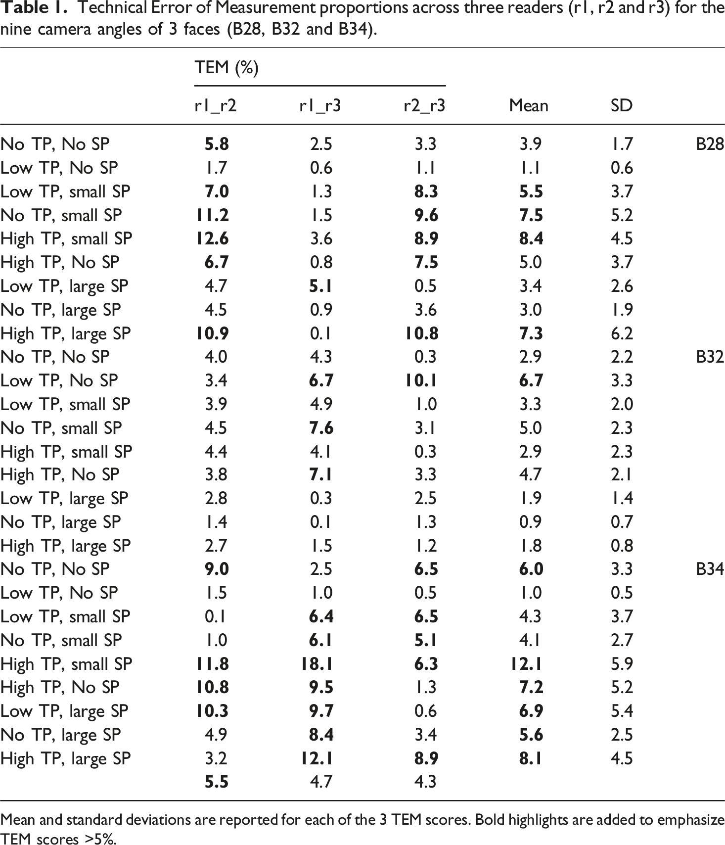
Mean and standard deviations are reported for each of the 3 TEM scores. Bold highlights are added to emphasize TEM scores >5%.

TEM scores >5% are highlighted in bold. No observable trends associated with camera angle can be identified. There is an approximately 5% technical error of measurement between the three readers across all 19 PtP measurements (r1_r2 = 5.5%, r1_r3 = 4.7%, r2_r3 = 4.3%). Overall, this demonstrates that reader defined error is not a major factor in variation and that with additional training it is expected that this could be improved. The readers used in this study (except for reader 1) were student interns deliberately provided with minimal instruction as to the identification of facial landmarks. Interobserver error is not uncommon in anthropometric studies with some studies showing facial measurement error rates across readers as high as 20% (Kouchi et al., 1999). Others suggest that the variation between readers can render some studies invalid (Bennett and Osborne, 1986). Research by Omari et al. (Omari et al., 2021) using similarly trained readers to this study observed similar rates of error with only a single reader measuring above the acceptable 5% error. It should also be noted that the images used in this study were relatively high quality and landmarks like Glabella and Nasion were relatively simple to pinpoint. Older, pixelated, and poor-quality images, such as those from cases pre-dating high resolution digital imaging will likely show greater reader variation.

Individual differentiation

Dot-plots for each of the ratios are shown in Supplemental Figures 1 and 2. Each dot-plot corresponds to one PtP measurement with the vertical axes representing one of 19 PtP measurements that was used to generate the ratio of the two. There are noticeable missing data where the PtP measurement is divided by itself as the ratio will always be 1 and was removed so as not to skew results.

Data used to generate dotplots in Supplemental Figures 1 and 2 are contained in Supplemental Table 1, listing each of the ratios, along with their calculated mean and CV (n = 27 per ratio). The highest CV for any ratio of PtP measurements was 38.7%, being from $\frac{L I - G N ’}{N - P N}$ . This represents the ratio of measurements from the labiale inferius (LI, bottom of bottom lip) to the gnathion (GN, chin tip) and the nasion (N, least protruding point between forehead and nose) to pronasale (PN, tip of nose). Because the N-PN measurement is taken from parts of the face with differing three-dimensional depths, it is more susceptible to changes in camera angle. This is likely an effect of the multiple camera angles and explains the large variability when N-PN is used to generate a ratio. This is discussed in further detail later in this manuscript and all ratios comprising of N-PN have herein been removed from the results.

The data from Supplemental Table 1 was truncated to show only those ratios with a CV >15% and further ordered from highest to lowest for clarity in Table 2.

Table 2.

Point to point ratios ranked by CV as highest to lowest in variability.

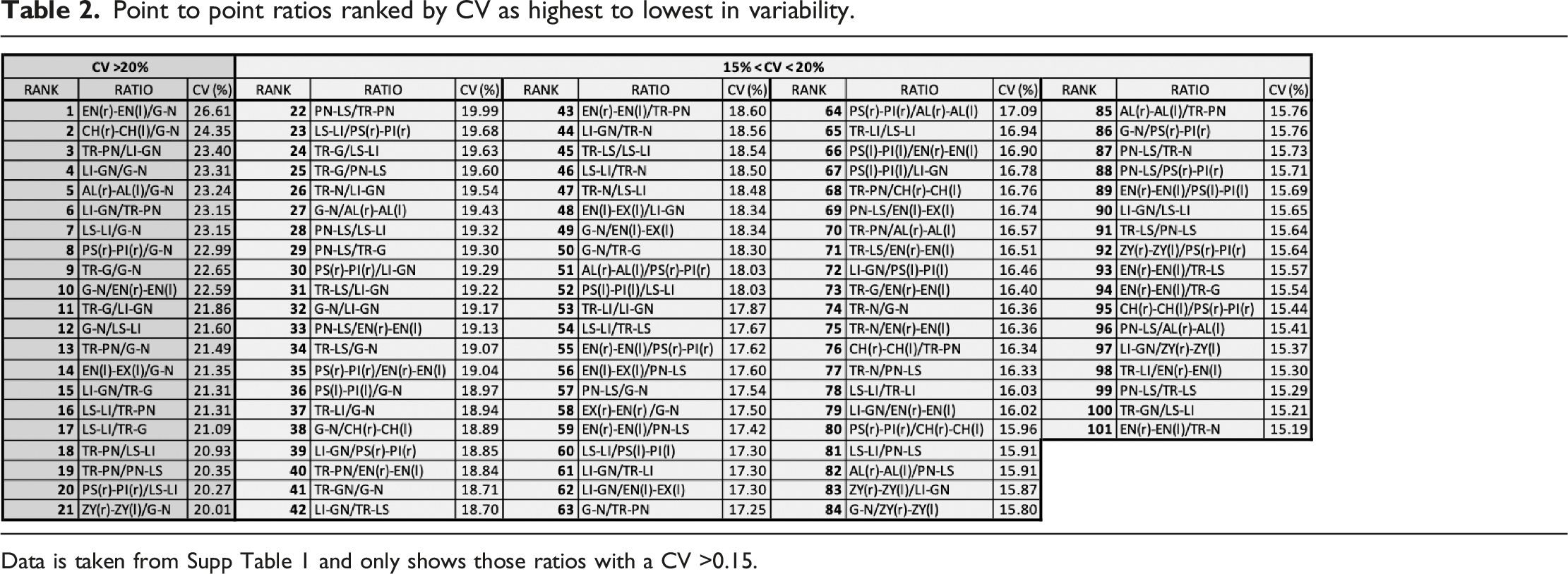
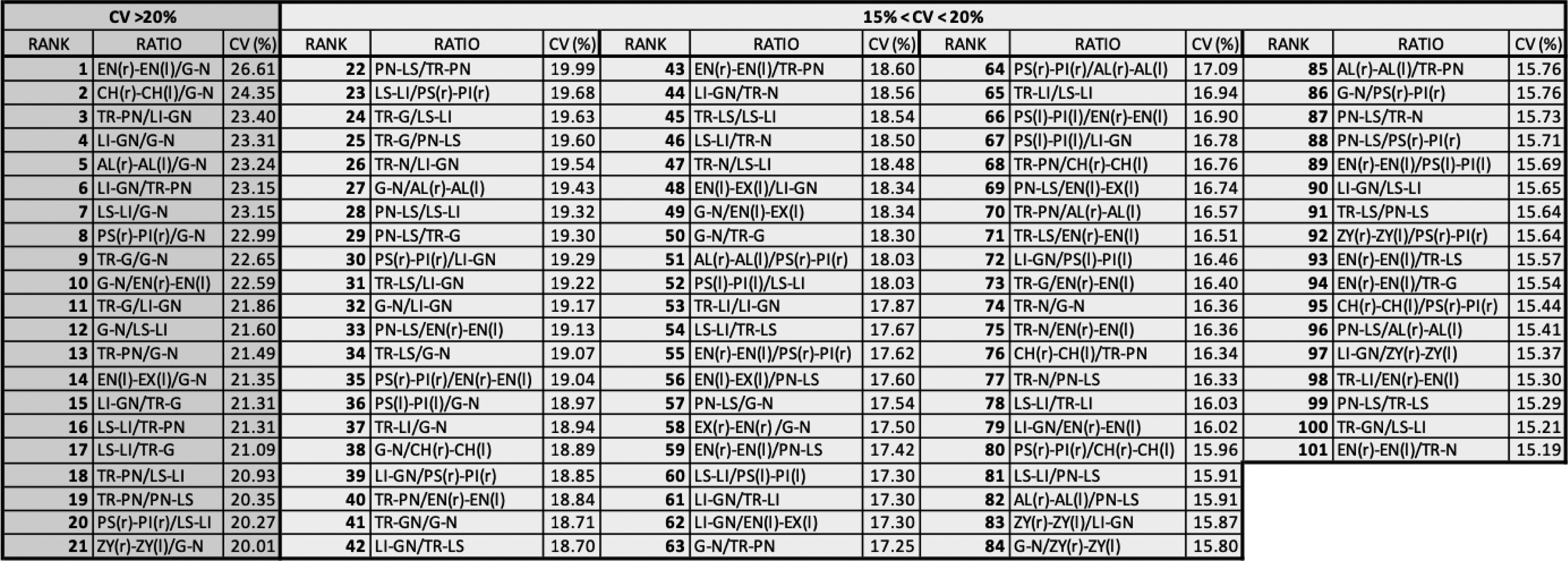
Data is taken from Supp Table 1 and only shows those ratios with a CV >0.15.

A CV of greater than 20% was observed for 21 ratios. A further 80 ratios resulted in CVs greater than 15%, but lower than 20%. These 101 PtP measurement ratios show the greatest variation across the nine camera angles, for three random faces. From this small participant set (n = 3), these ratios appear to offer the most utility in defining variation between individuals. In progressing with this technique, however, it is recommended that these are further tested against a larger database of faces to verify their validity in determining true individual variation. These three faces were selected randomly and clearly appear different but it could be argued that they are also more similar than a larger age, ethnicity and sex population range. There are also a number of repeated ratios within this set whereby the denominator and numerator are reversed, providing a ratio that is merely the inverse. These are further highlighted in later sections of the results. It is also likely that camera angle is influencing the CV scores, meaning that not all variation is due to true differences between the individual persons, and instead may be a feature of intra-person difference attributed to the camera angles.

Identifying ratios with a high and low susceptibility to changes in camera angle

A selection of the point-to-point data arrays is shown in Figure 3. In this example, there are three arrays shown, coinciding with one reader, and the collated CV data across all point-to-point measurements for all nine facial angles. Left to right, they represent B28, B32 and B34, respectively.

Each cell contains a pooled CV for one point-to-point measurement divided by another to give a ratio as discussed in the data acquisition section of the methods. Across the top and left of each array are the various measurements, numbered 1–19 and coinciding with those in Figure 2. The black cells are where a single measurement has been divided by itself, and hence will always equal 1 and is excluded from analysis. Light green cells are those measurements with a low CV (<5%) and light red cells those with a high CV (>20%). In any row or column whereby more than 4 cells are coloured, the corresponding measurement has been flagged in dark red or dark green accordingly. An example, row 3 for B28, contains 10 CV results >20%, and hence measurement 3 is flagged in dark red. When transformed into a meaningful interpretation, this suggests that for this reader, the Nasion to Pronasale (N-PN) measurement was highly variable to camera angle differences as previously demonstrated. This was observed by Moreton and Morley (Moreton and Morley, 2011) when moving camera angle between 10° and 40° in the horizontal angle. Looking further to B32 and B34 (middle and right arrays), the trend is similar. These data, when compiled with the other two readers, are summarised and presented in Figure 4.

Figure 4.

Summarised CV data for all three readers, across all three faces. If a measurement contributed to a ratio with high or low CV, it is coloured in green (low CV, seen as robust to change in camera angle) or red (high CV, seen as susceptible to change in camera angle).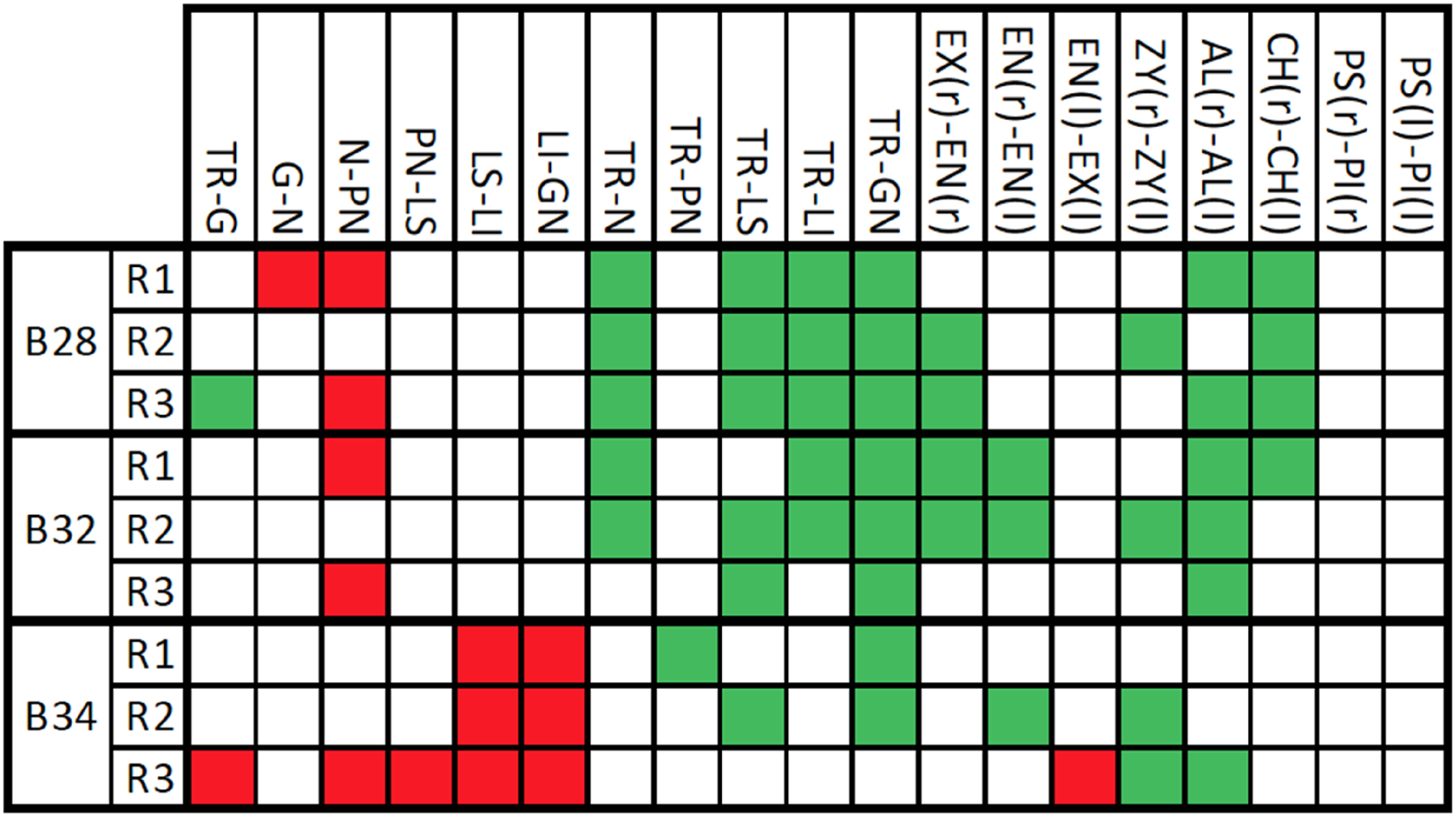

Visual trends are quickly identified from the results in Figure 4. Firstly, the trend previously illustrated in one reader’s results for Nasion-Pronasale is conserved across multiple readers and multiple faces. This was also previously flagged as bad data in the Individual Differentiation results. As previously mentioned, the inference to be drawn from this is that the N-PN measurement is highly susceptible to changes in camera angle. When considering that measurement with respect to a person’s face, this is not surprising as the N-PN line (Figure 2) represents one that in three dimensions runs from the nasion, located quite proximal to the coronal plane midline, to the pronasale (the tip of the nose), located distally from the coronal midline. Therefore, compared to directly front on, any alterations of facial angle will have a profound effect on that measurement as the nose tip moves in a greater arc.

A second identifiable trend is for the PtP measurements of Labiale superius to Labiale inferius (LS-LI) and Labiale inferius to Gnathion (LI-GN). LS-LI is more commonly understood as the measurement from top of the top lip to the bottom of the bottom lip. Similarly, LI-GN is the bottom of the bottom lip to the point of the chin. Both measurements showed high CVs for all three readers, but only for subject B34. When referring to the images, it was quickly identified that there was poor replication in the nine Yale images with respect to the candidate holding a neutral mouth position. As can be seen in Figure 5, in some images the candidate has a closed mouth and in others it is open. While these results demonstrate that the methods used in this study to detect variation are suitable, they invalidate those data points. No such trend is observed in B28 and B32, so it is inferred that the LS-LI and LI-GN measurements may be suitable for inclusion in future applications of this technique provided the position of the mouth is conserved.

Figure 5.

Four images from Yale set B34 illustrating the non-compliance of the participant in maintaining a neutral mouth pose. As can be seen, in some images the mouth is open exposing the teeth and others it is fully closed.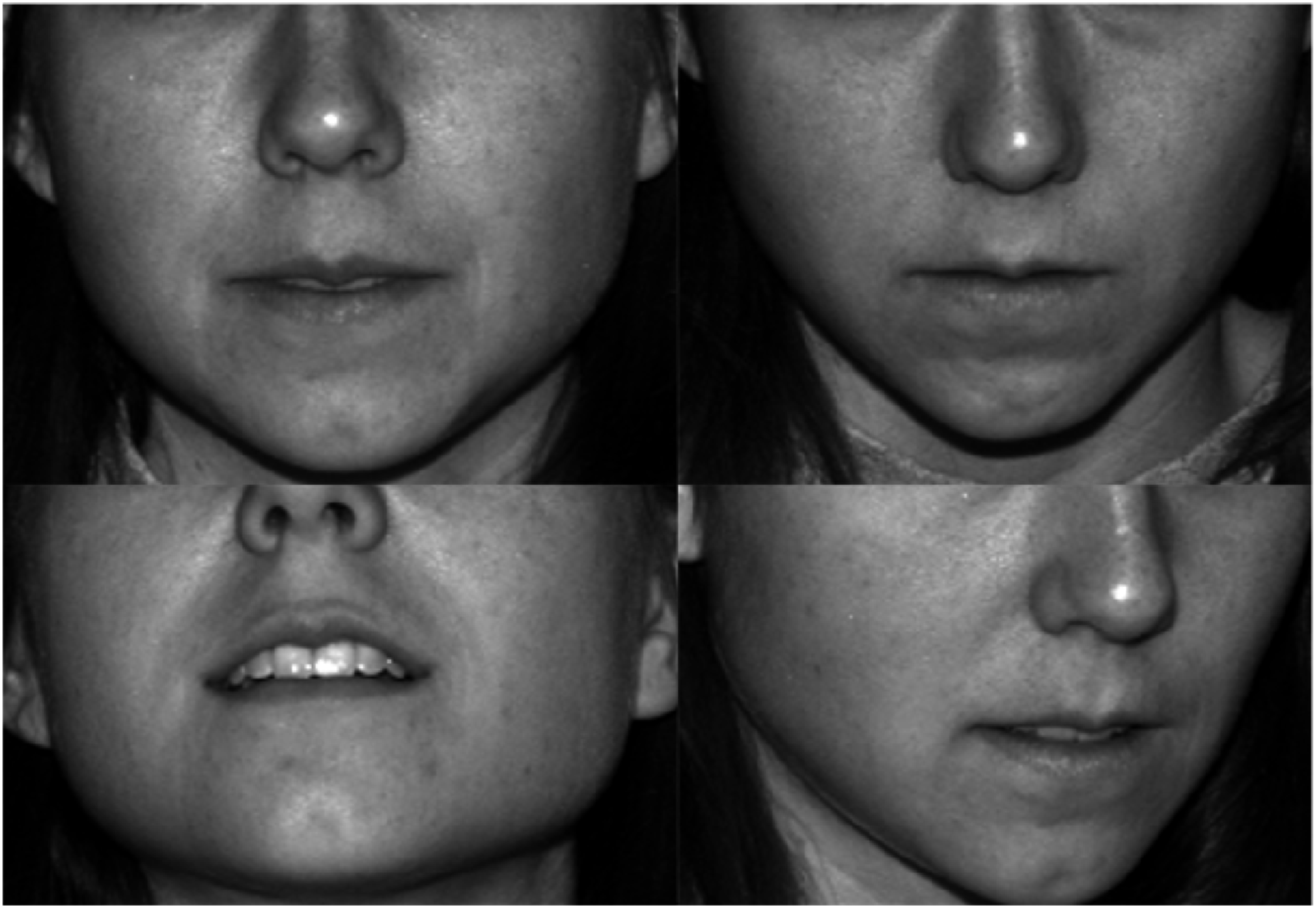

There are an additional 4 measurements that are flagged as having high CVs, namely TR-G, G-N, PN-LS and EN(l)-EX(l), but these data are only seen in either a single Yale face, or resulting from measurements of a single reader. Reader 3 contributes to 10 out of the total 15 flagged measurements, which may speak more to the ability of the reader to accurately plot landmarks than to the suitability of the landmarks themselves. As discussed, intra- and inter-rater reproducibility was approximately 5% or lower and could likely be improved with simple training beyond that provided in this study.

For the FSL analysis to have use for law enforcement, it needs to be robust to the input of victim photographs sourced from social media and personal and family photo collections. While best practice will always recommend the use of verified, official images such as passport or driver’s licence photos, they will not always be available, and this data shows how the effect of offset photographs can be mitigated.

Proof of concept test

A final test was conducted on the three faces, front on, to test the ability of these data points to differentiate the three faces. 101 ratios with a CV over >15% (arbitrarily defined) were chosen as a starting list. From that, any ratios containing the N-PN PtP measurement were removed as its variability has been demonstrated and explained by the previous tests. In addition to that, further ratios were excluded if they appeared twice within the list as an inverse fraction of each other, for example $\frac{T R - G}{G N}$ and $\frac{G N}{T R - G}$ . This left 55 ratios that are listed in Supplemental Data 2.

With these 55 ratios, a PCA plot was generated and is shown in Figure 6. The plot demonstrates an even spread of the three faces, suggesting that the model sufficiently resolves the differences between these participants’ biometric variation. To better understand what specific data points were driving the variation between the three faces, a heatmap was generated and is shown in Figure 7.

Figure 6.

PCA scores plot of three faces, B28, B32 and B34 using the 55 PtP ratios. Unit variance scaling is applied to rows; SVD with imputation is used to calculate principal components (PCs). X and Y axis show PC1 and PC2 that explain 75.8% and 24.2% of the total variance, respectively. N = 3 data points.

Figure 7.

Heatmap illustrating data variation in the three faces. Unit variance scaling is applied to rows; SVD with imputation is used to calculate principal components (PCs). X and Y axis show PC1 and PC2 that explain 75.8% and 24.2% of the total variance, respectively. N = 3 data points.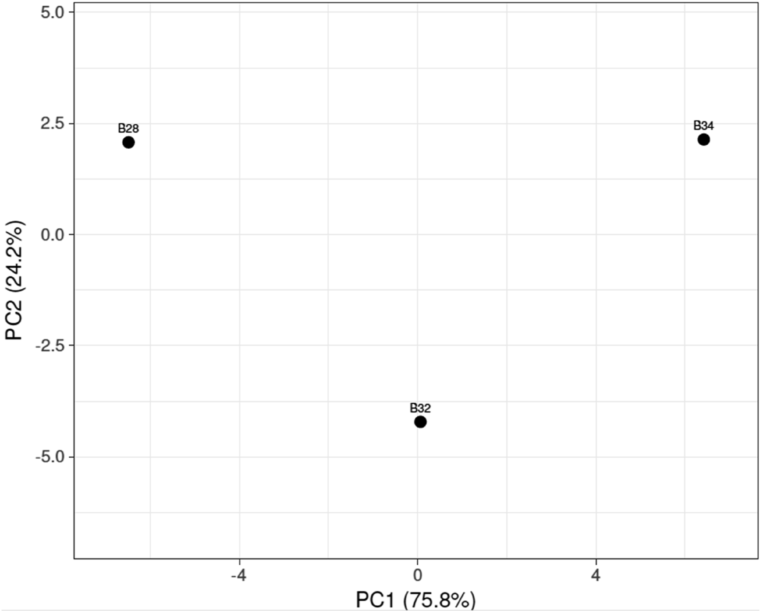

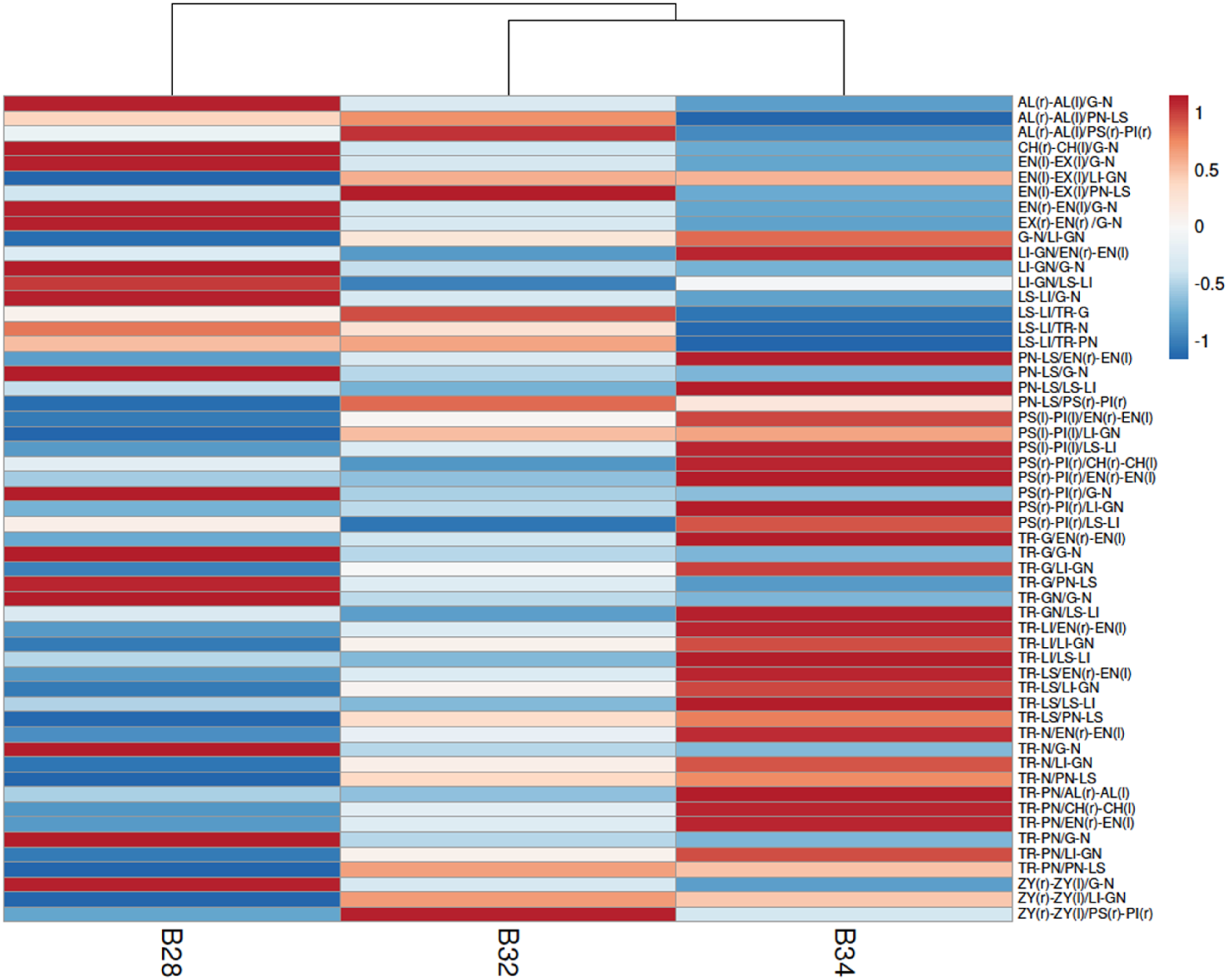
Variation between each individual is driven by different ratios. B28 and B32 differences are due to large variation (shown by red colouration adjacent to blue in Figure 7, with darker indicating higher variance) in $\frac{L I - G N}{L S - L I}$ , $\frac{PN - LS}{G - N}$ , $\frac{P S (r) - P I (r)}{G - N},$ $\frac{T R - G}{G - N}, \frac{T R - G N}{G - N}$ , $\frac{T R - N}{G - N}$ , $\frac{T R - P N}{G - N}$ , $\frac{E N (l) - E X (l)}{L I - G N},$ $\frac{P N - L S}{P S (r) - P I (r)}$ , $\frac{T R - P N}{P N - L S}$ , $\frac{Z Y (r) - Z Y (l)}{L I - G N}$ and $\frac{Z Y (r) - Z Y (l)}{P S (r) - P I (r)}$ . Commonalities seen in these ratios are those including the PtP measurements from G-N (in six ratios), LI-GN (in 3 ratios), PS(r)-PI(r) (in 3 ratios). Put simply, the vertical regions of the eye and chin are those most different between these two faces.

For B32, compared to B34 differences are owing to large variation in $\frac{A L (r) - A L (l)}{P S (r) - P I (r)}, \frac{E N (l) - E X (l)}{P N - L S}, \frac{L S - L I}{T R - G}, \frac{L S - L I}{T R - P N},$ $\frac{L I - G N}{E N (r) - E N (l)}, \frac{P N - L S}{L S - L I}, \frac{P S (r) - P I (r)}{C H (r) - C H (l)},$ $\frac{P S (r) - P I (r)}{E N (r) - E N (l)}$ , $\frac{P S (r) - P I (r)}{L S - L I},$ $\frac{T R - G N}{L S - L I},$ $\frac{T R - L I}{L S - L I}, \frac{T R - L S}{L S - L I},$ and $\frac{T R - P N}{A L (r) - A L (l)} .$ Commonalities seen in these ratios are those including the PtP measurements from LS-LI (in seven ratios) and PS(r)-PI(r) (in 4 ratios). For this pairing, the vertical height of the lips/mouth is the most different between these two faces with eye height also contributing.

Finally, for B28, compared to B34 differences are owing to large variation in $\frac{A L (r) - A L (l)}{G - N}$ , $\frac{C H (r) - C H (l)}{G - N}, \frac{E N (l) - E X (l)}{G - N}, \frac{E N (r) - E N (l)}{G - N}, \frac{E X (r) - E N (r)}{G - N}, \frac{L I - G N}{G - N}, \frac{L S - L I}{G - N}, \frac{L S - L I}{T R - N}$ , $\frac{P N - L S}{E N (r) - E N (l)}, \frac{P N - L S}{G - N}$ , $\frac{P S (r) - P I (r)}{G - N}$ , $\frac{T R - G}{G - N}, \frac{T R - G}{P N - L S}, \frac{T R - G N}{G - N}, \frac{T R - N}{G - N}, \frac{T R - P N}{G - N}, \frac{Z Y (r) - Z Y (l)}{G - N}, \frac{E N (l) - E X (l)}{L I - G N}, \frac{G - N}{L I - G N}, \frac{P N - L S}{E N (r) - E N (l)},$ $\frac{P S (l) - P I (l)}{E N (r) - E N (l)}, \frac{P S (l) - P I (l)}{L I - G N}, \frac{P S (l) - P I (l)}{L S - L I}, \frac{P S (r) - P I (r)}{L I - G N}$ , $\frac{T R - G}{E N (r) - E L (r)}, \frac{T R - G}{L I - G N}, \frac{T R - L I}{E N (r) - E N (l)}, \frac{T R - L I}{L I - G N}, \frac{T R - L I}{L S - L I}$ , $\frac{T R - L S}{E N (r) - E N (l)}, \frac{T R - L S}{L I - G N}, \frac{T R - L S}{L S - L I}, \frac{T R - L S}{P N - L S}, \frac{T R - N}{E N (r) - E N (l)}, \frac{T R - N}{L I - G N}, \frac{T R - N}{P N - L S}, \frac{T R - P N}{A L (r) - A L (l)}, \frac{T R - P N}{C H (r) - C H (l)}, \frac{T R - P N}{E N (r) - E N (l)}$ and $\frac{T R - P N}{L I - G N}$ . Commonalities seen in these ratios are those including the PtP measurements from G-N (in 14 ratios), LI-GN (in 10 ratios), PN-LS (in six ratios), LS-LI (in five ratios), TR-N (in five ratios), TR-PN (in five ratios), EN(r)-EN(l) (in seven ratios), and TR-G (in 4 ratios).

The data show that B28 and B34 are more different than any other pair used in this study, with this supported by the tree linking B32 and B34 as closer in similarity than to B28 (Figure 7). For this pairing, the greatest variation came from the vertical regions of the forehead, lips and chin as well as horizontal variation in the spacing of the eyes. Observing these two faces, the differences are not immediately obvious (Supplemental Figure 3). The ability of this revised FSL method to detect variation (and conversely, similarity) shows promise. For future studies, the 55 ratios used in this research should be applied to test known SMC victim data for verification of clustering with PCA. Inclusion of randomly selected “outgroups” from a similar database to the Yale set should assist in demonstrating its effectiveness. While highly speculative, it stands to reason that the minute similarities between victim faces may help understand childhood triggers of the sexually motivated subset of criminals in associating victim similarities to a paternal or maternal actor.

It is important to note that forensic techniques of this type are not akin to the evidentiary value of DNA evidence in linking victims of crime to offenders. Face Similarity Linkage, at best, may provide an intelligence tool to investigators seeking to link previously unrecognised victims of SMC. Once this first connection has been established, they may deploy additional, more robust investigative techniques to support their hypotheses. Additional research is needed to demonstrate the ability of the FSL technique in actual sex crime victim image sets.

Conclusion

Face Similarity Linkage, first detailed in Hackett et al. (Hackett et al., 2020), was presented as a rudimentary way to identify similarities between SMC victims. This research has developed the technique to a digital method, capable of potential automation with artificial intelligence but still enabling manual processes amenable to any law enforcement unit. Its robustness has been tested and optimised to minimise the effect of camera angle that is unlikely to be overcome with the use of victim images from family and social media. Using simple instructions to untrained personnel, error rates of around 5% were achievable which indicates that further improvement can be made with training. In this test, random, unrelated faces were shown to be very different by PCA plotting of 55 optimal facial geometric ratios.

Supplemental material

Supplemental Material - Development of face similarity linkage for the attribution of intelligence links in unsolved sexually motivated serial homicide

Supplemental Material for Development of face similarity linkage for the attribution of intelligence links in unsolved sexually motivated serial homicide by Brendan Chapman, David Keatley, John Coumbaros, Garth Maker in The Police Journal

Footnotes

ORCID iDs

Brendan Chapman

David Keatley

Funding

The authors received no financial support for the research, authorship, and/or publication of this article.

Declaration of conflicting interests

The authors declared no potential conflicts of interest with respect to the research, authorship, and/or publication of this article.

Supplemental material

Supplemental material for this article is available online.

Note

References

Adobe Inc. (2004) Adobe Photoshop 2020 (21.1). Peachpit Press. Available at: https://www.adobe.com/products/photoshop.html.

Belongie

Kriegman

Ramamoorthi

(2001) Yale Face Database B. Online Database.

Bennett

Osborne

(1986) Interobserver measurement reliability in anthropometry. Human Biology 58(5): 751–759. https://www.jstor.org/stable/41463808

Cornwell

Law Smith

Boothroyd

, et al. (2006) Reproductive strategy, sexual development and attraction to facial characteristics. Philosophical Transactions of the Royal Society B: Biological Sciences 361(1476): 2143–2154. https://doi.org/10.1098/rstb.2006.1936

Facial Identification Working Group (2012) Guidelines for Facial Comparison Methods Version 1.0. In 02.02. https://fiswg.org

Flores

MRP

Machado

CEP

Gallidabino

, et al. (2019) Comparative assessment of a novel photo-anthropometric landmark-positioning approach for the analysis of facial structures on two-dimensional images. Journal of Forensic Sciences 64(3): 828–838. https://doi.org/10.1111/1556-4029.13935

Galterio

Shavit

Hayajneh

(2018) A review of facial biometrics security for smart devices. Computers 7(3): 37. https://doi.org/10.3390/computers7030037

Hackett

Keatley

Chapman

(2020) Face similarity linkage: a novel biometric approach to sexually motivated serial killer victims. Expert Systems 37(6): e12597. https://doi.org/10.1111/exsy.12597

Hall

Chapman

(2026) Domestic and sexual violence in Australia: Current evidence and the potential role of forensic science. Forensic Science International: Synergy 12: 100665. Available at: https://doi.org/10.1016/j.fsisyn.2026.100665

10.

Hargrove

(2019) Murder Accountability Project. Webpage.

11.

Hazelwood

Warren

(2003) Linkage analysis: modus operandi, ritual, and signature in serial sexual crime. Aggression and Violent Behavior 8(6): 587–598. https://doi.org/10.1016/S1359-1789(02)00106-4

12.

Huston

Levinger

(1978) Interpersonal attraction and relationships. Annual Review of Psychology 29(1): 115–156. https://doi.org/10.1146/annurev.ps.29.020178.000555

13.

Jain

Ross

Prabhakar

(2004) An introduction to biometric recognition. IEEE Transactions on Circuits and Systems for Video Technology, Video Technol 14(1): 4–20. https://doi.org/10.1109/TCSVT.2003.818349

14.

Johns

O’Toole

Keel

, et al. (2008) Serial Murder: Multi-Disciplinary Perspectives for Investigators. Federal Bureau of Investigation.

15.

Kelly

Lynes

(n.d.) The Dark ‘Flâneur’: Re-Theorising Serial Murder Through the Ultra-realist Lens.

16.

Kouchi

Mochimaru

Tsuzuki

, et al. (1999) Interobserver errors in anthropometry. Journal of Human Ergology 28(1–2): 15–24. https://doi.org/10.11183/jhe1972.28.15

17.

LaBrode

(2007) Etiology of the psychopathic serial killer: an analysis of antisocial personality disorder, psychopathy, and serial killer personality and crime scene characteristics. Brief Treatment and Crisis Intervention 7(2): 151–160. https://doi.org/10.1093/brief-treatment/mhm004

18.

Labuschagne

(2014) The use of linkage analysis evidence in serial offense trials. In Crime linkage: Theory, research, and practice. Boca Raton, FL: CRC Press, 197–224.

19.

Langlois

Kalakanis

Rubenstein

, et al. (2000) Maxims or myths of beauty? A meta-analytic and theoretical review. Psychological Bulletin 126(3): 390–423. https://doi.org/10.1037/0033-2909.126.3.390

20.

Linedecker

(1997) Smooth Operator: The True Story of Seductive Serial Killer Glen Rogers. St. Martin’s Press.

21.

Lisak

Miller

(2002) Repeat rape and multiple offending among undetected rapists. Violence & Victims 17(1): 73–84. https://doi.org/10.1891/vivi.17.1.73.33638

22.

Mark

Herbenick

(2014) The influence of attraction to partner on heterosexual women’s sexual and relationship satisfaction in long-term relationships. Archives of Sexual Behavior 43(3): 563–570. https://doi.org/10.1007/s10508-013-0184-z

23.

Martos

Valsecchi

Ibáñez

, et al. (2018) Estimation of 2D to 3D dimensions and proportionality indices for facial examination. Forensic Science International 287: 142–152. https://doi.org/10.1016/j.forsciint.2018.03.037

24.

Metsalu

Vilo

(2015) ClustVis: a web tool for visualizing clustering of multivariate data using principal component analysis and heatmap. Nucleic Acids Research 43(W1): W566–W570. https://doi.org/10.1093/nar/gkv468

25.

Moreton

Morley

(2011) Investigation into the use of photoanthropometry in facial image comparison. Forensic Science International 212(1): 231–237. https://doi.org/10.1016/j.forsciint.2011.06.023

26.

Omari

Hunt

Coumbaros

, et al. (2021) Virtual anthropology? Reliability of three-dimensional photogrammetry as a forensic anthropology measurement and documentation technique. International Journal of Legal Medicine 135(3): 939–950. https://doi.org/10.1007/s00414-020-02473-z

27.

Penton-Voak

Perrett

(2000) Female preference for male faces changes cyclically: further evidence. Evolution and Human Behavior 21(1): 39–48. https://doi.org/10.1016/S1090-5138(99)00033-1

28.

Penton-Voak

Jones

Little

, et al. (2001) Symmetry, sexual dimorphism in facial proportions and male facial attractiveness. Proceedings of the Royal Society B: Biological Sciences, Ser B Biol Sci 268(1476): 1617–1623. https://doi.org/10.1098/rspb.2001.1703

29.

Perrett

Lee

Penton-Voak

, et al. (1998) Effects of sexual dimorphism on facial attractiveness. Nature 394(6696): 884–887. https://doi.org/10.1038/29772

30.

Rule

(2018) The Stranger Beside me (First Gall). Gallery Books.

31.

Schlesinger

(1998) Pathological narcissism and serial homicide: rewiew and case study. Current Psychology 17(2–3): 212–221. https://doi.org/10.1007/s12144-998-1007-6

32.

Winter

Lemeire

Meganck

, et al. (2013) Comparing the predictive accuracy of case linkage methods in serious sexual assaults. Journal of Investigative Psychology and Offender Profiling 10(1): 28–56. https://doi.org/10.1002/jip.1372

Supplementary Material

Please find the following supplemental material available below.

For Open Access articles published under a Creative Commons License, all supplemental material carries the same license as the article it is associated with.

For non-Open Access articles published, all supplemental material carries a non-exclusive license, and permission requests for re-use of supplemental material or any part of supplemental material shall be sent directly to the copyright owner as specified in the copyright notice associated with the article.

0.00 MB

2.04 MB