
Abstract
A whole branch of theoretical statistics devotes itself to the analysis of clusters, the aim being to distinguish an apparent cluster arising randomly from one that is more likely to have been produced as a result of some systematic influence. There are many examples in medicine and some that involve both medicine and the legal field; criminal law in particular. Observed clusters or a series of cases in a given setting can set off alarm bells, the recent conviction of Lucy Letby in England being an example. It was an observed cluster, a series of deaths among neonates, that prompted the investigation of Letby. There have been other similar cases in the past and there will be similar cases in the future. Our purpose is not to reconsider any particular trial but, rather, to work with similar, indeed more extreme numbers of cases as a way to underline the statistical mistakes that can be made when attempting to make sense of the data. These notions are illustrated via a made-up case of 10 incidents where the anticipated count was only 2. The most common statistical analysis would associate a probability of less than 0.00005 with this outcome: A very rare event. However, a more careful analysis that avoids common pitfalls results in a probability close to 0.5, indicating that, given the circumstances, we were as likely to see 10 or more as we were to see less than 10.
Cases of Sally Clark, Lucia de Berk, and Lucy Letby
Our focus here is relatively narrow. We do not re-open past trials in order to re-examine any contentious issues. Nor do we dwell on many of the potentially related statistical matters. The discussion is limited to a specific problem, a problem sharply exemplified by the cases of the 3 women who provide the heading for this section. All 3 women were convicted of murder.
In each of the 3 cases the murder investigations were not initiated as a result of tangible evidence that a murder had even taken place. Instead, the investigations were consequent to an observation that there was something most unusual about an observed cluster of deaths. The clusters involved infants and neonates, babies whose precarious lives depended fully on adult care. The loss of life was deemed to indicate a lack of such care and, potentially, a lack so great as to suggest criminal intent. The question then becomes, who may be the person behind that intent. In the absence of any material evidence the only thing that could be described as being most unusual was the size of the clusters, the numbers of deaths. Since high risk babies were involved in the cases of Letby and de Berk, a certain number of deaths were to be anticipated. What was unusual was the size of the number itself, a number that would be considered to be unusual in the light of the fact of it arising with a vanishingly small probability under normal circumstances. That observation puts the spotlight on a key principle, the principle being an answer to the simple question: How do we decide what is“an unusually high” number? How can it be measured?
Unusually high can only be measured in terms of probability, a way to quantify the discrepancy between the observed number and one that we might anticipate observing under some given set of circumstances. While a discrepancy of order 2 would not have been particularly large in the case of neonates in intensive care, in the case of apparently healthy babies, in the same family environment, two deaths as opposed to a tiny expected number barely distinguishable from zero, may appear to be so large as to trigger a criminal investigation. This was the background to the case against the British solicitor Sally Clark. In her case the prosecution’s expert witness plunged head first into the “lottery blunder” described below deriving a probability for the observed outcome of the two deaths of her children that was incorrect by very many orders of magnitude. Not only did the expert witness plunge headfirst into the lottery blunder, he managed to bring the jury with him. They made the same mistake. With hindsight it is difficult to believe that such a wildly inaccurate statistical assessment went without successful challenge. Whatever challenges were made they were clearly not convincing enough and Sally Clark was sentenced to life imprisonment, a conviction that was upheld following appeal close to one year later in October 2000. Doubts on the soundness of the conviction grew 1 and resulted in a second appeal. This was successful and in 2003 her conviction was overturned after having spent more than three years in prison. She died shortly afterwards aged 42.
Dutch nurse Lucia de Berk was found guilty of 4 murders and 3 attempted murders on a neonatal ward in the Netherlands. This was in 2003. In 2004, on appeal, her situation worsened and she was subsequently found guilty of 7 murders and 3 attempted murders. She was sentenced to a full life term with no possibility of parole. There was no material evidence connecting Lucia de Berk to the deaths. The conviction leaned upon circumstantial evidence, notably an unusually high number of deaths that seemed difficult to explain and an apparently strong degree of correlation associating her presence on the ward with the shifts during which the deaths occurred. A law psychologist was called upon by the prosecution to determine the statistical probability that we ought associate with the observed high number of deaths. 2 His calculation took pains to overcome some well known statistical hurdles but, once again, failed entirely to avoid the lottery blunder described below. The result was a calculation incorrect by many orders of magnitude. An error heavy with consequences for, as argued by the Dutch professor of criminal law Theo de Roos, 3 the conviction of de Berk could hot have been obtained without it. After spending over six years in prison Lucia de Berk was fully exonerated in 2010.
In August 2023, Manchester Crown Court in England, UK found Lucy Letby guilty of the murder of 7 babies; neonates being treated at the Countess of Chester Hospital. She has been sentenced to a full life term. The main news outlets describe her as the worst child serial killer in modern history. Both the prosecution and the defence agreed that there was no material evidence linking Ms Letby to the crimes. Circumstantial evidence was provided instead. Expert witnesses were called upon to use their medical knowledge to unravel a host of facts and to identify, with as little doubt as possible, who could be the person responsible for the 7 deaths. Interestingly, and in parallel with the Lucia de Berk case, some personal jottings appended to a diary led to both nurses being seen in a very poor light. Although this may have been the closest the prosecution came to tangible evidence it was not in fact presented at trial. Also in striking parallel with the Lucia de Berk case the prosecution argued that there was a strong degree of correlation associating nurse Letby’s presence on the ward with the corresponding shifts at which several incidents occurred.
Had it been believed that no murders ever took place then we would not be looking for someone to blame. That explanation was however discounted. and it was thought that the murders did take place. Even so, at the times of death, and for years beyond that, the babies were believed to have died from natural causes. There were no signs that any baby had been murdered. No indication of any kind that something was amiss in the care of these babies. So why was that conclusion put into doubt? For no compelling reason other than a statistic: the high number of observed deaths, a number taken to be high when contrasted with what would have been anticipated. A statistic! A very weighty one! One which both the prosecution and the defence agreed to be more than suspiciously high. Indeed, so high that both sides could only see foul play as being at the origin of the deaths. That common conclusion was the first step in a series of steps that ended with the Letby conviction.
Might there though be grounds for questioning that first step, for asking ourselves: How compelling is the evidence that any crime at all has been committed, Could the observed number of deaths have occurred by chance alone? While chance is always possible: Is it plausible? If there are doubts about that first step then would that not weaken our confidence in all of the subsequent, and indeed consequent, steps.
Our purpose here is not to re-examine the trial of Lucy Letby. Nor is it to present any new arguments for that specific case. At the time of writing, the author believes that the prosecution is considering bringing further charges, the defence is preparing an appeal and a public inquiry has been announced to provide some answers to the families involved. In consequence we cannot say very much here that directly may have a bearing on any part of this process. We can though consider that first step in an abstract way in its own right, that is to say without specific reference to any particular trial and purely focused on numbers alone. In the absence of any precise definition can we ask ourselves the question: What constitutes a “spike” in the death rate. Not only that but if a spike is believed present then how plausible is it for the spike to have arisen by the play of chance. How likely is that?
This is of great importance. Cases, strikingly similar to the de Berk and Letby cases have occurred in the past. New cases are all but certain to appear in the near future. Both the prosecution and defence, diligently pursuing their objectives as adversaries, have at the same time a much deeper and shared objective; to find the truth. The opinion expressed here is that that objective can only be helped by giving due consideration to some elementary statistical arguments. These arguments are very much at the heart of the matter and however much we can understand the court’s desire to minimize highly technical discussions, the arguments can not be avoided.
Probability: How unlikely is unlikely? How rare is rare?
In any decision making context—legal decision making being no exception—everyday notions such as likely, unlikely, uncommon or rare, will hold a central place in the discussion. We may deem as rare or unlikely something that is potentially observable, or that has already been observed, This is an everyday concept. Everyday in that almost everyone would use such terms and most everyone would have a good idea of what they mean. At least what they mean to them. Can we though be more precise? Here is where our difficulties begin, and they are no small difficulties.
Probability theory is a formal means for addressing issues dealing with uncertainty. Before we can even begin however we need to accept the idea that there is such a thing as uncertainty, that uncertainty exists. Easier said than done. From real courtroom situations to TV fictional dramas, how often do we hear “his DNA was found at the crime scene.” In contrast, how often do we hear, “the 12 genetic markers analyzed in the sample found at the crime scene matched the same 12 genetic markers of the accused: Serious grounds for suspicion since, for a random sample taken from the population, such a degree of matching would be expected to be rare, say less than one case in one million. The first statement admits no possibility of uncertainty. The second not only admits a possibility of uncertainty but immediately opens the door to questions concerning the one in one million probability. Where did that come from? Is it the result of simple counting, i.e., the observed number of rare matches divided by some very large sample? In which case has the question of sampling error been addressed. Or is it the result of some model? Since any model is no more than a collection of assumptions, then just what are these assumptions? How reasonable are they? Has there been any study of model validity? Are we talking about a whole population, all ethnicities put together in one mixed bag. If so, and the ethnicity of the accused is known, then ought we not talk about random samples from that subgroup—necessarily less heterogeneous—rather than sampling from the whole population? The resulting estimate may turn out to be orders of magnitude greater than the one in one million originally calculated.
The more sophisticated the technique the greater the reluctance to admit the presence of uncertainty. Rather than a more precise wording to the argument we still continue to hear, “the suspect’s DNA was found at the crime scene.” Such hesitancy to concede the inevitability of uncertainty dates to well before DNA testing when we would often hear that some suspect’s fingerprints were found at the crime scene. Almost never did we hear that several characteristics of fingerprints, found at the crime scene, correspond to those of the suspect. The latter statement opens the door to an acknowledgment of uncertainty and, consequently, for the need to find plausible quantification of that uncertainty. A statistician will tell you that any such endeavor equates to a significant challenge. But, if such numbers are to be used in evidence, then they need backing up. They cannot be just pulled out of the air.
Probability: The lottery blunder
The most common blunder in statistical reasoning is what we might call the “lottery blunder,” also referred to here as the “lottery fallacy.” The mistake is very obvious to see, despite which, this was the very blunder that weighed so heavily in all of the convictions described above. Why the term lottery blunder? Because, in the case of a lottery, the reasoning is so obviously flawed.
Here’s how it goes: since the probability of winning the lottery is, say, less than one in ten million then the winner must have cheated. We can all see the flaw in that argument. Indeed, they may have cheated but that is no doubt unlikely and, how unlikely it is, becomes immediately apparent when the calculation is carried out correctly. A correct calculation would use the calculus of probability to sum over all the entrants to the lottery. The fault in the logic, as clear to those with no mathematical training as to those with such training, is in the neglecting of the role played by the many participants in the lottery. The probabilistic sum ought involve all of the participants. Everyone would agree to that.
Suppose however our interest is on something seemingly very different: an observed spike in the number of deaths at one of some 200 health care facilities across the country. The average number of yearly deaths is about 2 but one center drew special attention to itself given a rate very far above average at 10 deaths. A close analysis of that center might show that the probability of seeing that many deaths is minuscule. Based on routine statistical calculations we can obtain a probability for such an occurrence as being less than 5 divided by 100,000. Small! Is it correct though? In fact that common calculation is making the very same mistake as above, the lottery blunder. It is less obvious however and many would struggle to understand why an accurate analysis would consider not just what has been observed at that particular center but would aim, in some way, to involve in the calculation of the results from all centers. The logical mistake is the same. The context is quite different and one where logical clarity is less commonly shared. We return to this below.
At the heart of the lottery blunder is the failure to fully appreciate the major distinction between the probability of a given situation resulting in some outcome, identified by the outcome itself, from that of the same situation prior to any knowledge of the outcome.
Probability: A spike in incidence rates
Let us not give any precise definition on what we mean by a “spike” in incidence rates but, instead, we consider a made-up illustration. Suppose that there are 200 health care centers each having, for the sake of argument, very similar numbers of patient entry. This number could be well over one hundred and, on average, we anticipate seeing a quite small rate of incidence of death of about 2 per center. Under an independence assumption for the patients—certainly a reasonable first approximation—the basic probability law describing the observed number per center would be the Binomial and, for such a large potential number compared to the average rate, this is approximated to a very high degree of accuracy 4 by a Poisson law with mean 2. Let us work with this law.
One center stands out from the others in that what might be described as a spike in incidence of death is observed. Rather than the average of 2 or close to 2 deaths we see 10. How unusual is that? It appears to be an unlikely result given what we know and our question, a seemingly simple one, is what probability can be associated with that outcome? We can then use this calculated probability as a gauge of just how unusual, or not so unusual, are the 10 deaths we have observed. When this probability is small and close to zero it is not unreasonable to conclude that the 10 deaths were unlikely to have arisen by random sampling variation alone. Something else seems to be behind this unusually high number.
We can keep the mathematics to a minimum level but some notation will be helpful. So, let us then denote the number of deaths observed in Center
The Poisson law for counts is fully defined by its mean alone,
4
in this case 2, and using numerical methods or available software including on-line Poisson calculators, we find that
5
The center under scrutiny was not chosen randomly. It was chosen because of the observed high incidence rate of death, in fact among the very highest, if not the highest itself, out of the total of 200 centers. If not then we can assume that other centers would have attracted similar attention. Given that, and in order to not fall into the trap of the lottery blunder, ought we not focus our statistical attention on the quantity One important feature ignored in the above two sets of calculations is that of center heterogeneity. Both sets assume what is referred to by statisticians as independent and identically distributed variables, a statistical assumption translating a physical assumption - that conditions between different centers are taken to be essentially identical. This is clearly unrealistic. While the overall mean is 2 we would expect in practice, were we in a position to obtain enough observations over time, to observe differences between centers even if small. A host of factors could contribute to such heterogeneity. Socio-economic conditions could be expected to vary and these alone may play some role in the incidence rates.
7
Then there are environmental conditions that may differ, even within any given center, year in year out, as well as operational factors such as staff shortages, training differences to mention just a few. So, although the overall mean may remain at 2 there may exist some variability between centers. For a Poisson law based on i.i.d. observations, the mean and the variance are the same and equal to the within center variance.
8
The overall variance however will be greater than that and will correspond to the simple expression:
A certain number of observations can be made. The first and foremost is that, depending on our working assumptions, we find results that are so fundamentally different as to lead to entirely different conclusions. The first tells us that there appears to be strong evidence for some non-random influence to be at work, the third that the result is wholly compatible with having arisen purely by chance. So, which is it? The first explanation makes the classical lottery blunder and, as such, can be dismissed outright. The second does not make this mistake but ignores the fact that not all centers are identical. The third shows that even a very modest amount of variability between the centers will result in a much larger probability estimate for the observed result. We can conclude with some assurance that not only are the 10 cases observed compatible with random sampling but that, in the immediate future, say the next two or three years, we can be very confident in predicting that as great a number will occur again. It would not be likely to occur at the same center but would be likely to occur at one of the 200 centers. We will say more on this in the conclusion below.
Critical analysis
Our purpose here is to underline the impact of some of the most common statistical errors when attempting to analyze observed clusters. It is not to carry out any in-depth statistical analysis of the data. That said, we have presented a very limited statistical analysis of the observations at hand and, as for any such analysis, it is important to identify any assumptions being made. In turn that will lead to two important and related tasks. The first is to assess just how plausible, and realistic, the assumptions may be. The second task is to study what we might, in an informal mathematical language, refer to as smoothness: we would like for small departures from the assumptions to result in small departures in the findings. 9 The above calculations lean on an assumed Poisson model. How reasonable is that? For situations in which counts can theoretically range from 0 to a large number and the anticipated counts are small in comparison then, for a Poisson law to hold, all that we need is independence between counts. 8 Within a center this will usually be a very reasonable and workable assumption. Even so, we can imagine small departures from independence, for example when observing the mortality of neonates in a center and, among them, a small proportion of twins. Some potentially shared genetic fragility may put a small dent in the independence assumption. Even if present however the impact would be negligible.
Our second major assumption was in the choice of a log-normal distribution 8 to characterize the distribution of Poisson means between centers in the presence of center heterogeneity. The most obvious first choice - a Gaussian distribution - was ruled out since it would allow for the possibility of negative average counts. A log-normal law only allows for positive counts. However, unlike the Poisson law for the counts themselves, we have no physical argument in favor of a log-normal law. Given that, it makes sense to investigate the impact of several choices of possible probability laws. Since the array of choices is without limit, the investigation itself is limited. Nonetheless, a study of widely contrasting choices can provide some reassurance. We looked at a number of discrete distributions with probability weights chosen so that the overall mean of the rates remains fixed at its average 2, and spread over the lower integers in varying ways. Added to this we considered some established alternatives to the log-normal law constrained to have a mean of 2. None of these alternative choices for describing the variability between centers had any significant impact on the outcomes.
One choice that will have a significant impact on our findings is the ratio of within-center variance to between-center variance. The illustration chose the background (within center) variability to be twice that of the between-center variability. This is, of course, a wholly arbitrary assumption. We know the impact of this assumption is strong and, indeed, that is one of our main arguments. Often within center variability will be ignored which, in practice, means that we take it to be zero. This led us to conclude that
Neglected information, Bayesian thinking, and causality
The statistical errors described above arise as a consequence of not taking into account important and relevant information, specifically the fact that the events considered to be quite exceptional were identified after they had taken place and not before. Also, the simple observation that we would expect some differences, even if small, between centers. Such information will have a very significant impact on the probabilities that we wish to calculate and require some technical expertise if we wish to obtain more accurate results. Notwithstanding the conceptual challenge to the lay person’s understanding, we can find more everyday examples where failing to account for relevant information will lead us astray. A precise calculation of probabilities is not needed to see this. The case of Barry George, convicted of the murder of a popular journalist and subsequently acquitted at a second trial illustrates the importance of the weighting of evidence. Finding firearm residue on George’s clothing matching that found at the crime scene would have seemed most unusual for a randomly chosen individual. Yet, in George’s case, this neglects very important information: George was a member of a gun club so that a re-weighting of the evidence results in an “unusual” becoming a much less unusual.
And in some cases, plain common sense will do no lesser a job than delicate calculations. Table 1 shows a summary of the shifts during which different nurses at a clinic were on duty. This included a nurse suspected of murder and the shifts shown are those where a death or serious event occurred that had triggered the investigation of the nurse. Such a chart was used in evidence at the trials of both Lucia de Berk and Lucy Letby. The suspected nurse stands out very clearly from the other nurses and, a cursory glance, may lead us to believe that the suggestion of guilt is strong. However, the data is incomplete. All it actually shows is that when the suspected nurse was on duty she was …on duty. When all of the data is shown and none of the information neglected, that is all of the deaths and incidents, and not just those involving the nurse under investigation, then a very different picture emerges. a picture that is much less compelling.
A record identical in form to ones shown at the trials of Letby and de Berk.
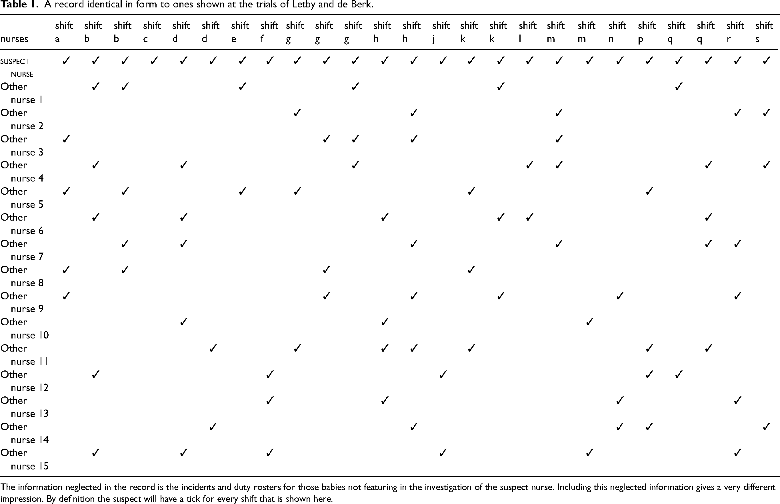
The information neglected in the record is the incidents and duty rosters for those babies not featuring in the investigation of the suspect nurse. Including this neglected information gives a very different impression. By definition the suspect will have a tick for every shift that is shown here.
None of the above addresses directly the question of causality. The calculated probabilities described above can, if we so wish, be incorporated into a more complete analysis that attempts to break down the sources of variability into possible causes.10,11 The numbers alone tell us a great deal but it is not unreasonable to want to go further and to ask the question: Can some of that overall variability in death rates be decomposed into a part that can be attributed to a cause and the remaining component to be deemed unexplained. This corresponds to a very standard and widely accepted approach to statistical analysis. For example, in a neo-natal unit, the higher rates of incidence may be attributable in part to known risk factors 12 in the local population (exposure to alcohol, drugs etc) as well as conditions in the health care facility such as staff shortages, training discrepancies or general hygiene.
A fuller analysis would do its best to address these issues. Bayesian inference and causal inference are scientific disciplines that have attracted a great deal of attention over the last few decades. Much progress has been made and these techniques can no doubt help us to obtain a more thorough analysis. While this would be well beyond the scope of this current communication, we can nonetheless indicate how such analyses can provide some simple and valuable insights. At its most elementary level Bayesian thinking would want us to explicitly account for the plausibility of different potential causes. 10 This is rarely done, and to the writer’s knowledge, there are no established examples in the legal field. We might consider relative plausibility to equate to the ratio of likelihoods, the numerator corresponding to an assumption that randomness, possibly translating varying conditions between centers, explains the observations while the denominator is based on an assumption that a murderer is on the loose. An analysis that ignores the relative plausibility of these two assumptions cannot in fact avoid their impact and amounts to assigning an equal weight of 0.5 to both assumptions. A Bayesian analysis would make every effort to obtain the most realistic relative weightings to the two assumptions. Since it is all but impossible to know the weightings precisely there is clearly a degree of arbitrariness in their choice, a feature to the Bayesian approach that is often a source of criticism. However, the choice is inevitable and it seems preferable to discuss any choices rather than try to avoid them which does no more than attribute equal weightings to either choice.
On a deeper level, Bayesian thinking would turn our attention away from a problem that is largely irrelevant and put the focus on what truly matters. In the motivating examples to this article, in all cases, the observed events were most unusual. The probability of their occurrence would be tiny. Yet, they did occur. That we know. So why even bother to consider how probable or not it was that such an occurrence could take place. Such information has technical value in our calculations but as information to a juror or a police detective, it has no value. The events did take place so let’s start there. In the case of Sally Clark we can all agree that something very unusual happened. But happened it did and the relevant question - the one the Bayesian would ask - is, given that fact, how likely is one explanation when compared to another explanation. The numbers change dramatically and instead of discussing estimated probabilities involving millions or trillions we would be looking at much more manageable, and interpretable, quantities in single or double digits at most. Different assumptions regarding the potential explanations would have an impact on the outcome but not necessarily a very large one and, in all cases, would put us in a position to carry out an enlightened and meaningful discussion about the plausibility of competing explanations.
Conclusion
The illustration highlights how easily we can be led astray when carrying out a statistical assessment of observed clusters or series of events. Great care is needed and an important first step is to be able to steer away from some common errors, the lottery fallacy being the most misleading. In many cases that step alone is enough to save us from coming to a conclusion not warranted by the observations. Going beyond that there are two main approaches to trying to make sense of clusters or series of events that, at first inspection, seem to be very unusual.
The first approach, outlined earlier in this paper, is to closely examine two issues. Are we calculating the probability of the relevant event? For the 10 observed cases in one of 200 centers, identified retrospectively by the number of cases itself, the relevant outcome is not the number of deaths at any randomly chosen center but is the maximum number over all 200 centers. As we saw, this makes a significant difference. The second issue deals with any working assumptions that are being made. How realistic are they? We saw that a small, and very plausible, amount of variability among centers would, once more, have a large impact on our estimated probability. It would be hard to argue that some variability is not a more realistic assumption than no variability.
The second approach sets out to present a related but altogether different probability. This is the Bayesian approach and considers the probabilities of the events themselves to be only of indirect interest. We take the outcome, the number of deaths for example, to be fixed and known. Given that fact, the probability we wish to study is the one describing the potential causes and explanations that may have given rise to that outcome. In the case of, say, a series of events in a pediatric intensive care unit we might all agree that something quite unusual has taken place. How unlikely such a series may be is though not where our attention should be focused. Instead, given say a first explanation—this is a random occurrence largely explicable in terms of natural variation reflecting conditions on different wards—and a second explanation—this is the result of a deliberate act of harmful intent, then the odds of the explanation being the first or the second can be evaluated. Some challenging technical issues are involved but, in many ways, it appears that we are trying to answer the most relevant question. That said, even in an age of artificial intelligence, there is something rather disturbing about deciding whether or not there is evidence of criminal intent based on the balance of probabilities alone. Material evidence is surely preferable. However, if probabilities are permitted to enter the discussion then that discussion should be as broad as possible.
Many legal professionals would say that these concepts will not be readily understood by the average juror. And that the court ought steer clear from such technical issues of probability, relying instead on material evidence. Few would argue against that. Unless that is, the prosecution’s case and the police investigation lean to any degree on the relative plausibility, or implausibility, of an observed cluster. When that happens then such technical issues cannot be avoided. Patient communication and careful explanation will enable many if not all of the jurors to grasp whether, and to what extent, a conclusion they are asked to make leans wholly or partially on the lottery fallacy. Without doubt it would be preferable to avoid technical probabilistic arguments in the courtroom. But, if one side chooses to introduce them, then the opposing side needs to know how to adequately prepare their response.
Footnotes
Acknowledgment
The author is grateful to the reviewers and editors for suggestions that have led to a more focused, yet more complete, presentation. I am also very grateful to Sean Devlin for technical assistance and to Alexia Iasonos and Michel Broniatowski for many very helpful discussions.
Declaration of conflicting interests
The author declared no potential conflicts of interest with respect to the research, authorship, and/or publication of this article.
Funding
The author received no financial support for the research, authorship and/or publication of this article.