Sage Journals: Discover world-class research

Abstract

This tutorial paper introduces two approaches to modeling tongue contour data obtained with DeepLabCut using multivariate generalized additive models (MGAMs) and multivariate functional principal component analysis (MFPCA). For each method, we present a fully commented analysis of two illustrative data sets: VC coarticulation in Italian and Polish, and consonant emphaticness in Lebanese Arabic. All the materials (inlcuding data and code) are available in the research compendium of the tutorial at https://github.com/stefanocoretta/mv_uti. We conclude by discussing advantages and disadvantages of the two methods (MGAM and MFPCA) and we recommend researchers to prefer MFPCA over MGAM as an initial step for modeling tongue contours.

Keywords

Ultrasound tongue imaging multivariate statistics Generalized Additive Models functional principal component analysis articulation

1 Introduction

Ultrasound tongue imaging (UTI) is a non-invasive technique that allows researchers to image the shape of the tongue during speech at medium temporal resolution (30–100 frames per second, Epstein & Stone, 2005; Stone, 2005). Typically, the midsagittal contour of the tongue is imaged, although 3D systems exist (Lulich et al., 2018). Recent developments in machine-learning-assisted image processing has enabled faster tracking of estimated points on the tongue contour (Wrench & Balch-Tomes, 2022).

Wrench and Balch-Tomes (2022) have trained a DeepLabCut (DLC, Mathis et al., 2018) model to estimate and track specific flesh points on the tongue contour and anatomical landmarks as captured by UTI. The model estimates 11 “knots” from the vallecula to the tongue tip, plus three muscular-skeletal knots (the hyoid bone, the mandible base and the mental spine where the short tendon attaches). See Figure 1 for a schematic illustration of the position of the tracked knots. An advantage of DLC-tracked data over the traditional fan-line coordinate system is that (in theory) specific (moving) flesh points are tracked rather than simply the intersection of the tongue contour with fixed radii from the fan-line system. This makes DLC-tracked data resemble data obtained with electromagnetic articulography (EMA). The downside is that the tongue contour is represented by 11 freely moving points, which can move in any direction in the midsagittal two-dimensional space captured by UTI, and this requires more advanced statistical approaches than those commonly employed to analyze tongue contour data.

Figure 1.

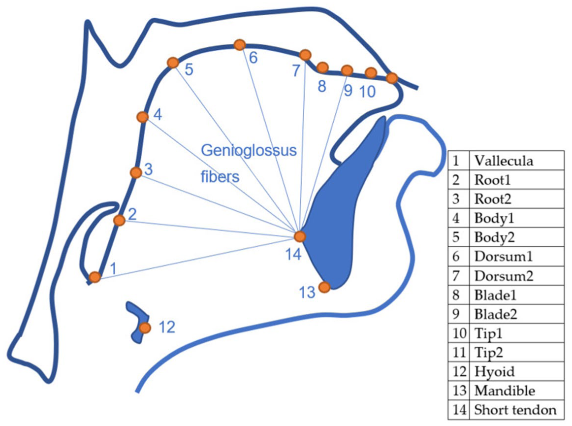
Schematic representation of the knots tracked by DeepLabCut. CC-BY Wrench and Balch-Tomes (Wrench, 2024).

Classical ways to analyze tongue contour data obtained from a fan-line system, like SS-ANOVA (Chen & Lin, 2011; Davidson, 2006) and Generalized additive models using Cartesian coordinates are not appropriate with DLC-tracked data, due to the tongue contour “curling” onto itself along the root and due to the vectors of movement of the knots. The first point is illustrated in Figure 2: the plot shows the DLC-tracked points (in black) of the data from a Polish speaker and the traced tongue contours based on the points (see Section 2.1 for details on the data). The contours clearly curl onto themselves along the root (on the left of the contour). The red smooths represent a LOESS smooth, calculated for Y along X. This approach miscalculates the smooth for the back half of the tongue, simply because there are two Y values for the same X value, and the procedure, in that case, returns something like an average of the two values. Generalized additive models using Cartesian coordinates work on the same principle and hence would produce the same type of error.

Figure 2.

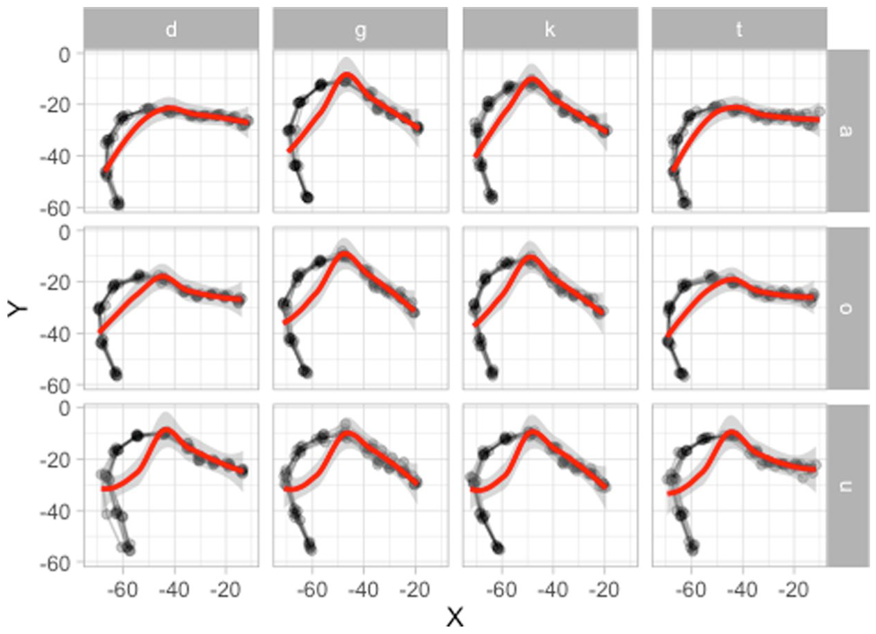
Illustrating tongue contours curling up along the root. The estimated smooths in red fail to capture the curl.

Coretta (2018b) and Coretta (2019) suggest using polar coordinates with generalized additive models to overcome the shortcomings of Cartesian coordinates. While using polar coordinates with DLC-tracked data would work mathematically, as shown in Gubian (2025), it is less ideal from an articulatory perspective: a polar-based fan-line system with a single origin fails to capture the vectors of movement of the individual knots estimated by DLC. Figure 3 illustrates this point with DLC-tracked data from a Lebanese speaker. The figure shows the tracked points from the entire data set of that speaker and each of the 11 DLC-tracked knots is shown in a different color. The knots appear to move along well-defined vectors defined by eye inspection (with the exception of the fifth knot, which can be regarded as the pivot knot), represented in the figure by black segments. The vectors of articulatory movement make sense in light of the muscular anatomy of the tongue (Honda, 1996; Hoole, 1999; Pettersson & Wood, 1987; Wrench, 2024). The polar radii in gray radiate from a manually selected origin with coordinates (100, 30). While the radii would correctly capture the position of each knot on the bi-dimensional space, the modeling of displacement is constrained by the direction of the radii. Figure 3 shows that one same knot intercepts different radii across different snapshots, making it impossible to associate anatomically defined positions on the tongue to radial coordinates, which eventually defies the purpose of DLC tracking. We don’t consider this constraint to be fatal, but any multivariate model, like MGAMs or MFPCA, allows for a more accurate depiction of knot movement by removing such constraints.

Figure 3.

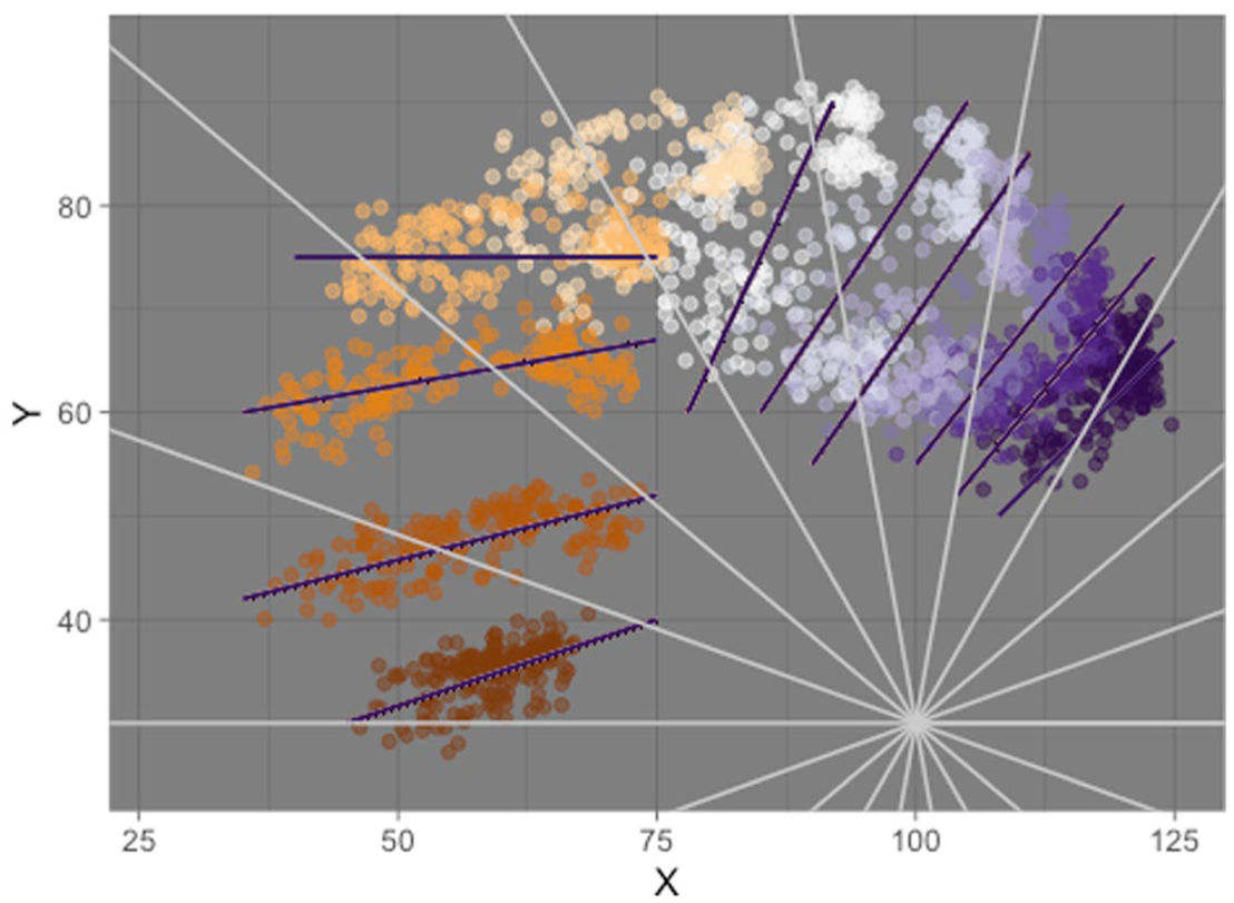
Illustrating vectors of articulatory movement versus polar coordinates. Colored points are individual DLC-tracked points (knots) on the tongue surface (each knot is in a different color, for a total of 11 knots). The white radial coordinates are chosen approximately to illustrate that they do not follow the movement vectors of the knots. The approximated movement vectors are represented by the dark lines (one for knot). The radial coordinates and movement vectors are based on eye-balling, not on calculation.

In this tutorial, we introduce two alternative methods to analyze DLC-tracked tongue contour data: multivariate generalized additive models (Section 2) and multivariate functional principal component analysis (Section 3). We will present the pros and cons of each method in Section 4, but to summarize we are inclined to recommend multivariate functional principal component analysis over multivariate generalized additive models due to the substantial computational overhead and reduced practical utility of the latter over the former. This tutorial illustrates how to conduct static analyses of tongue contours (i.e., modeling contours at specific time-points), but the techniques discussed here can be extended to dynamic (time-varying) analyses as shown in Gubian (2025). We follow two specific implementations generalized additive models and multivariate functional principal component analysis as provided by the mgcv package (Wood, 2006) and the MFPCA package (Happ & Greven, 2018; Happ-Kurz, 2022).

2 Multivariate generalized additive models

Generalized additive models (GAMs) are an extension of generalized models that allow flexible modeling of non-linear effects (Hastie & Tibshirani, 1986; Wood, 2006). GAMs are built upon smoothing splines functions, the components of which are multiplied by estimated coefficients to reconstruct an arbitrary time-changing curve. For a thorough introduction to GAMs we refer the reader to Sóskuthy (2021b); Sóskuthy (2021a); Pedersen et al. (2019); and Wieling (2018). Multivariate generalized additive models (MGAMs) are GAMs with more than one outcome variable.

As mentioned in Section 1, the data tracked by DeepLabCut consists of the position on the horizontal (x) and vertical (y) axes of 14 knots. In this tutorial, we will focus on modeling the tongue contour based on the 11 knots from the vallecula to the tongue tip. Figure 4 illustrates the reconstructed tongue contour on the basis of the 11 knots: the tongue in the figure is from the offset of a vowel [o] followed by [t], uttered by a Polish speaker (see Section 2.1).

Figure 4.

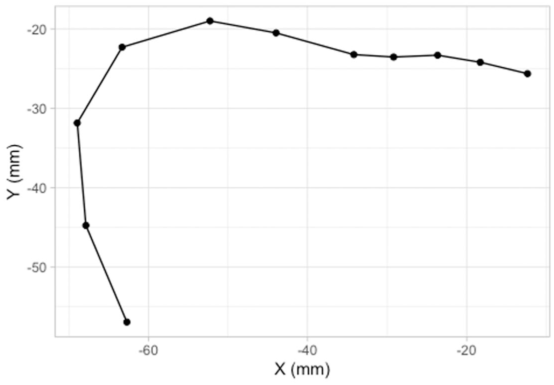
The 11 knots on the tongue contour taken from the offset of [o] followed by [t] (Polish speaker PL04, tongue tip to the right).

The same data is shown in Figure 5 in a different format. Instead of a Cartesian coordinate system of X and Y values, the plot has knot number on the x-axis and X/Y coordinates on the y-axis. The X/Y coordinates thus form “trajectories” along the knots. These X/Y trajectories can be modeled using MGAMs and multiple functional principal component analysis (MFPCA): in both cases, the X/Y trajectories are modeled as two variables changing along knot number. In this section, we will illustrate GAMs applied to the X/Y trajectories along the knots and how we can reconstruct the tongue contour from the modeled trajectories. We will use data from two case studies of coarticulation: vowel-consonant (VC) coarticulation based on consonant place in Italian and Polish, and consonantal articulation of plain versus emphatic consonants in Lebanese Arabic.

Figure 5.

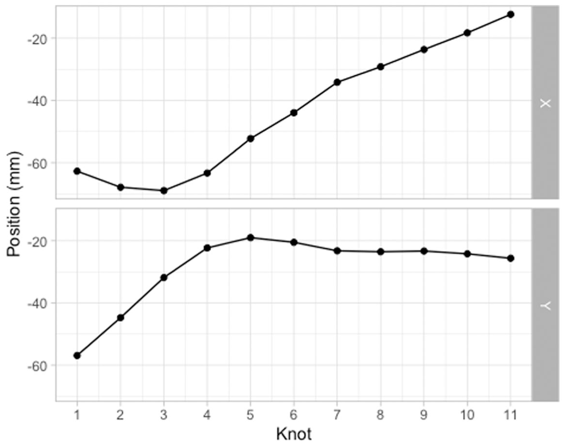
The horizontal and vertical positions of the 11 knots (same data as Figure 4).

2.1 VC coarticulation

The data of the first case study, Coretta (2018a), comes from Coretta (2020b) and has been discussed in Coretta (2020a) (the analysis in the latter concerned the position of the tongue root during the duration of vowels followed by voiceless or voiced stops; in this paper we focus on tongue contours at the vowel offset). The materials are /pVCV/ words embedded in a frame sentence (Dico X lentamente “I say X slowly” in Italian and Mówię X teraz “I say X now” in Polish). In the /pVCV/ words, C was /t, d, k, ɡ/ and V was /a, o, u/ (in each word, the two vowels were identical, so for example, pata, poto, putu). The data analyzed here is from 9 speakers of Italian and 6 speakers of Polish (other speakers were not included due to the difficulty in processing their data with DeepLabCut).

Video recordings of tongue ultrasound were obtained in Articulate Assistant Advanced™ (AAA, Articulate Instruments Ldt. 2011). Spline data was extracted using a custom DeepLabCut (DLC) model developed by Wrench and Balch-Tomes (2022). When exporting from AAA™, the data was rotated based on the bite plane, obtained with the imaging of a bite plate (Scobbie et al., 2011), so that the bite plane is horizontal: this allows for a common coordinate system where vertical and horizontal movement are comparable across speakers. Once the DLC data was imported in R, we manually removed tracking errors and we calculated z-scores within each speaker (the difference between the value and the mean, divided by the standard deviation). These steps are documented in the “Prepare data” notebook online, available at https://stefanocoretta.github.io/mv_uti/notebooks/01_prepare_data-preview.htm.

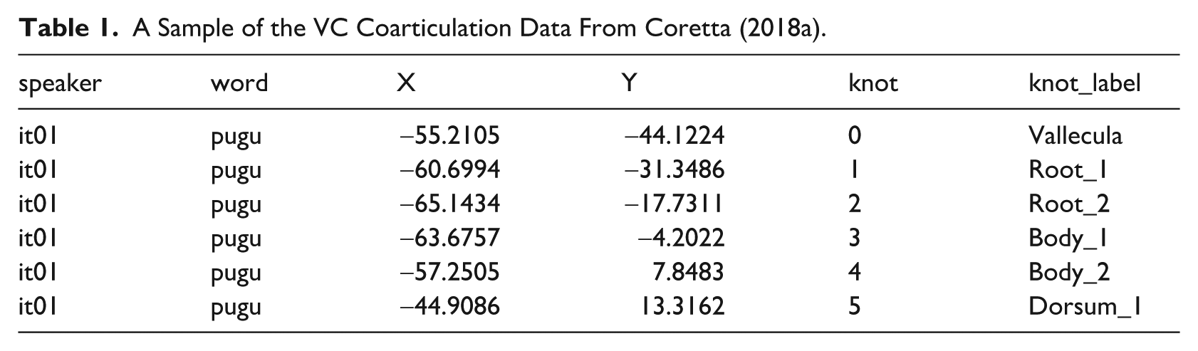
The following code chunk reads the filtered data. A sample of the data is shown in Table 1. Figure 6 shows the tongue contours for each individual speaker. It is possible to notice clusters of different contours, related to each of the vowels /a, o, u/. Figure 7 zooms in on PL04 (Polish): the contours of each vowel are colored separately, and two panels separate tongue contours taken at the offset of vowels followed by coronal (/t, d/) and velar stops (/k, ɡ/). Crucially, the variation in tongue shape at vowel offset (or closure onset) across vowels contexts is higher in the coronal than in the velar contexts. This is not surprising, giving the greater involvement of the tongue body and dorsum (the relevant articulators of vowel production) in velar than in coronal stops.

dlc_voff_f <- readRDS("data/coretta2018/dlc_voff_f.rds”)

Table 1.

A Sample of the VC Coarticulation Data From Coretta (2018a).

speaker	word	X	Y	knot	knot_label
it01	pugu	-55.2105	-44.1224	0	Vallecula
it01	pugu	-60.6994	-31.3486	1	Root_1
it01	pugu	-65.1434	-17.7311	2	Root_2
it01	pugu	-63.6757	-4.2022	3	Body_1
it01	pugu	-57.2505	7.8483	4	Body_2
it01	pugu	-44.9086	13.3162	5	Dorsum_1

Figure 6.

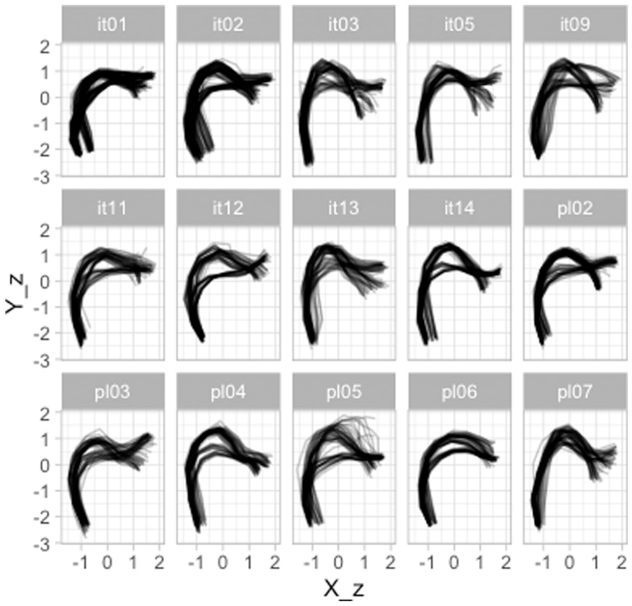
Tongue contours of nine Italian speakers and six Polish speakers, taken from the offset of the first vowel in /pCVCV/ target words.

Figure 7.

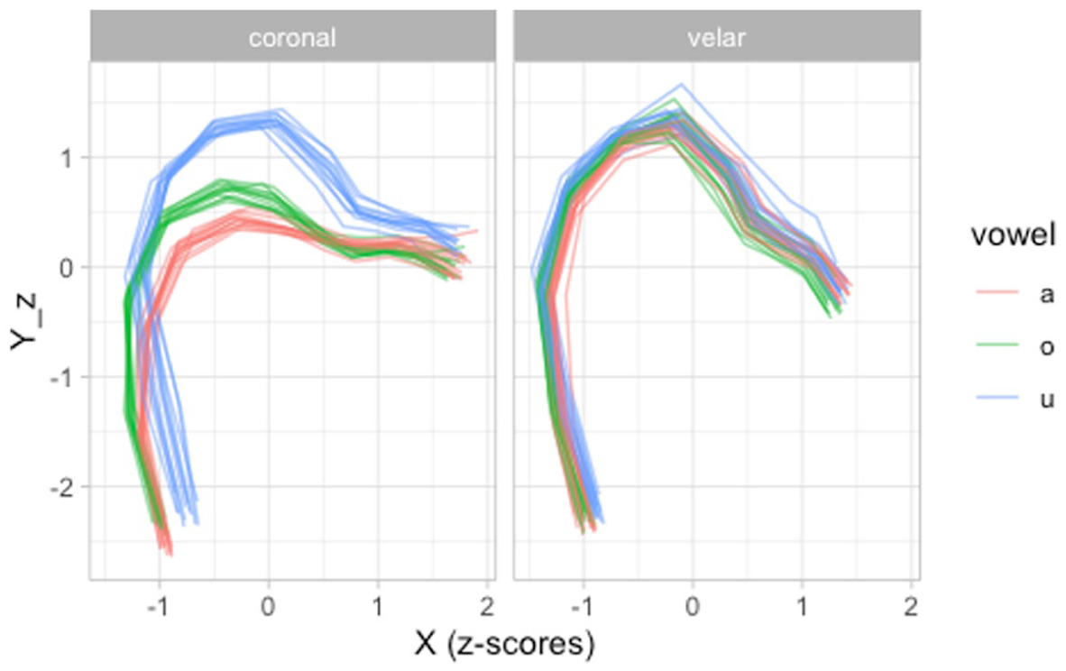
Tongue contours of PL04 (Polish) taken from the offset of vowels followed by coronal or velar stops. Tip is on the right.

We can now run a multivariate GAM to model the tongue contours. A multivariate GAM can be fitted by providing model formulae for each outcome variable (in our case, X_z and Y_z) in a list. For example list(y ~ s(x), w ~ s(x)) would instruct mgcv::gam() to fit a bivariate GAM with the two outcome variables y and w. The required family is mvn for “multivariate normal”: mvn(d=2) indicates a bivariate family (a multivariate family with two dimensions, that is, two outcome variables). In the model below, we are fitting a multivariate GAM to the z-scored X and Y coordinates. For both outcome variables, we include a smooth over knot (s(knot, . . .)) with a by variable vow_place_lang: this variable is built from an interaction of vowel, place and language.¹ We set k to 5: this will usually be sufficient for X/Y coordinates of tongue contours, since they are by nature not very “wiggly” (which would require a higher k). However, users are recommended to check whether k should be increased with the function gam.check() from the mgcv package (see documentation of the function for details). We also include a factor smooth over knot for speaker (the equivalent of a non-linear random effect) with s(knot, speaker, . . .): since language is a between-speaker variable, we use the interaction of vowel and place, vow_place, as the by variable.

library(mgcv)

voff_gam <- gam(

list(

X_z ~ vow_place_lang +

s(knot, by = vow_place_lang, k = 5) +

s(knot, speaker, by = vow_place, bs = “fs”, m = 1),

Y_z ~ vow_place_lang +

s(knot, by = vow_place_lang, k = 5) +

s(knot, speaker, by = vow_place, bs = “fs”, m = 1)

data = dlc_voff_f,

family = mvn(d = 2)

)

The model summary is not particular insightful. What we are normally interested in is the reconstructed tongue contours and in which locations they are similar or different across conditions. To the best of our knowledge, there isn’t a straightforward way to compute sensible measures of comparison, given the multidimensional nature of the model (i.e., only one or the other outcome can be inspected at a time; moreover, difference smooths, like in Sóskuthy (2021b) and Wieling (2018), represent the difference of the sum of the outcome variables, rather than each outcome separately, Michele Gubian pers. comm.) We thus recommend to plot the predicted tongue contours and base any further inference on impressionistic observations on such predicted contours. Alas, there is also no straightforward way to plot predicted tongue contours, but to extract the predictions following a step-by-step procedure, like the one illustrated in the following paragraphs.

First off, one has to create a grid of predictor values to obtain predictions for. We do this with expand_grid() in the following code chunk. We start with unique values of speaker, vow_place and knot (rather than just using integers for the knots, we predict along increments of 0.1 from 0 to 10 for a more refined tongue contour). We then create the required column vow_place_lang by appending the language name based on the speaker ID. Note that all variables included as predictors in the model must be included in the prediction grid.

# Create a grid of values to predict for

frame_voff <- expand_grid(

# All the speakers

speaker = unique(dlc_voff_f$speaker),

# All vowel/place combinations

vow_place = unique(dlc_voff_f$vow_place),

# Knots from 0 to 10 by increments of 0.1

# This gives us greater resolution along the tongue contour than just using 10 knots

knot = seq(0, 10, by = 0.1)

) |>

mutate(

vow_place_lang = case_when(

str_detect(speaker, “it”) ~ paste0(vow_place, “.Italian”),

str_detect(speaker, “pl”) ~ paste0(vow_place, “.Polish”)

)

With the prediction grid frame_voff we can now extract predictions from the model voff_gam with predict(). This function requires the GAM model object (voff_gam) and the prediction grid (frame_off). We also obtain the standard error of the prediction which we will use to calculate Confidence Intervals in the next step. Since we have used factor smooths for speaker, we now have to manually exclude these smooths from the prediction to obtain a “population” level prediction. We do this by listing the smooths to be removed in excl: note that the smooths must be named as they are in the summary of the model, so always check the summary to ensure you list all of the factor smooths. Finally, we rename the columns with the name of the outcome variables.

# List of factor smooths, to be excluded from prediction

excl <- c(

"s(knot,speaker):vow_placea.coronal",

"s(knot,speaker):vow_placeo.coronal",

"s(knot,speaker):vow_placeu.coronal",

"s(knot,speaker):vow_placea.velar",

"s(knot,speaker):vow_placeo.velar",

"s(knot,speaker):vow_placeu.velar",

"s.1(knot,speaker):vow_placea.coronal",

"s.1(knot,speaker):vow_placeo.coronal",

"s.1(knot,speaker):vow_placeu.coronal",

"s.1(knot,speaker):vow_placea.velar",

"s.1(knot,speaker):vow_placeo.velar",

"s.1(knot,speaker):vow_placeu.velar"

)

# Get prediction from model voff_gam

voff_gam_p <- predict(voff_gam, frame_voff, se.fit = TRUE, exclude = excl) |>

as.data.frame() |>

as_tibble()

# Rename columns

colnames(voff_gam_p) <- c(“X”, “Y”, “X_se”, “Y_se”)

Now we have to join the prediction in voff_gam_p with the prediction frame, so that we have all the predictor values in the same data frame. We do so here with bind_cols() from the dplyr package. Note that voff_gam_p contains predictions for each level of the factor smooths, despite these being excluded from prediction. If you inspect the predictions for different speakers, you will find that they are the same for the same levels of vow_place_lang: this is because the effects of the factor smooths were removed, so speaker has no effect on the predicted values. This means that you can pick any Italian and Polish speaker in the predicted data frame. We do so by filtering with filter(speaker %in% c(“it01”, “pl02”)), but any other speaker would lead to the same output. We also calculate the lower and upper limits of 95% confidence intervals (CI) for each coordinate. Note that you should interpret these CI with a grain of salt, because they are not truly multivariate, but rather represent the CI on each coordinate axis independently.

voff_gam_p <- bind_cols(frame_voff, voff_gam_p) |>

# pick any Italian and Polish speaker, random effects have been removed

filter(speaker %in% c(“it01”, “pl02”)) |>

# Calculate 95% CIs of X and Y

mutate(

X_lo = X - (1.96 * X_se),

X_hi = X + (1.96 * X_se),

Y_lo = Y - (1.96 * Y_se),

Y_hi = Y + (1.96 * Y_se)

) |>

# Separate column into individual variables, for plotting later

separate(vow_place_lang, c(“vowel”, “place”, “language”))

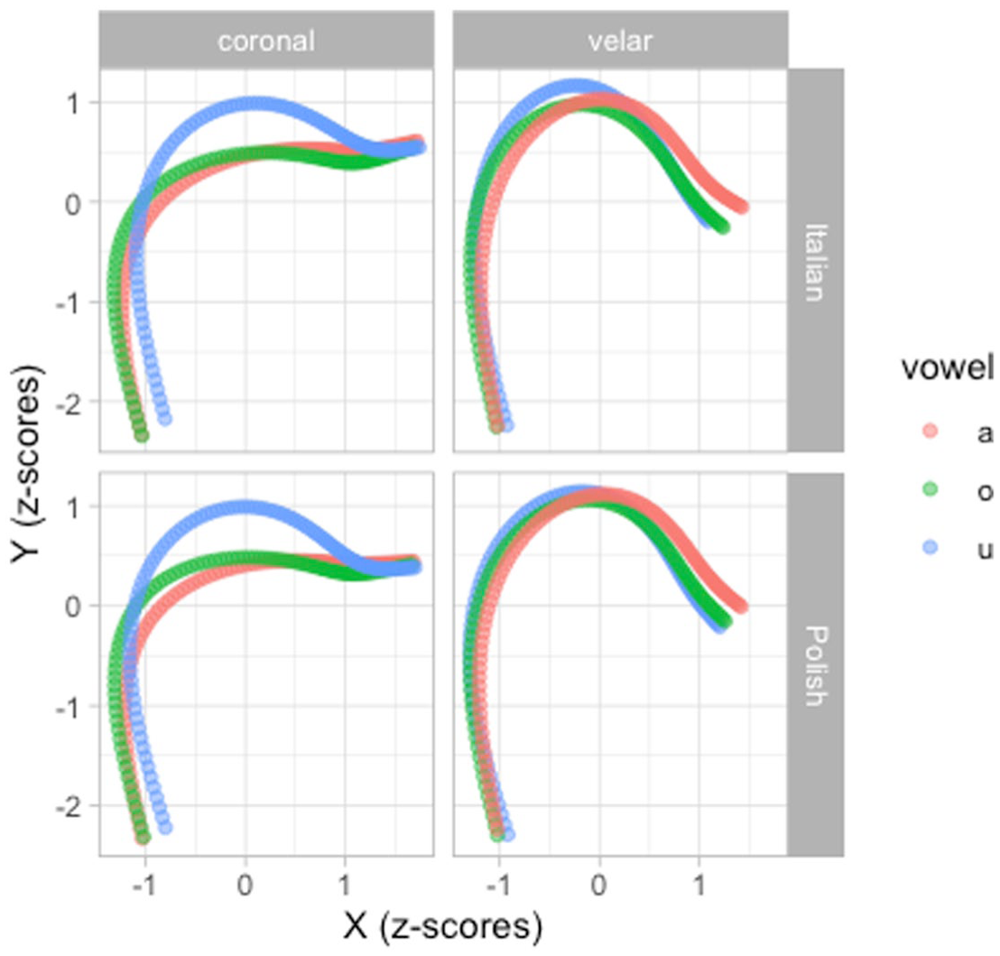
Figures 8 and 9 show the predicted tongue contours based on the voff_gam model, without and with 95% CIs respectively. As mentioned earlier, there isn’t a straightforward way to obtain any statistical measure of the difference between the contours on the multivariate plane, so we must be content with the figure.

Figure 8.

Predicted tongue contours based on a multivariate GAM. Uncertainty not shown.

Figure 9.

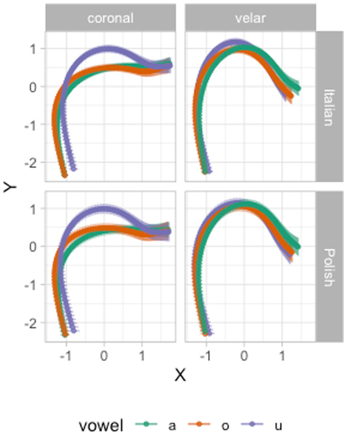
Predicted tongue contours based on a multivariate GAM, with 95% confidence intervals.

Figure 9 strongly suggests greater VC coarticulation on the C closure in coronal that in velar contexts. Moreover, the vowels /a, o/ have a similar coarticulatory effect on the tongue contour. With velar consonants, we observe less coarticulation from the preceding vowel (a possible explanation of this is given at the end of Section 3.1).

2.2 Emphaticness

The second case study is about consonant “emphaticness” in Lebanese Arabic. The data is from Sakr (2025). Lebanese Arabic is a variety of Arabic primarily spoken in Lebanon, where it is in constant contact with a number of Indo-European languages (primarily English and French, as vectors of education and business, see, for example, Shaaban & Ghaith, 1999), as well as the written standard form of Arabic known as Modern Standard Arabic (MSA). The relationship between Lebanese Arabic (LA) and MSA in Lebanon is one of diglossia (see, for example, Lian, 2022), where LA is spoken in most contexts, but not written, and MSA is the written variety, and therefore also primarily used for legal and official purposes.

Emphasis is a phonologically contrastive feature of Semitic languages. In most varieties of Arabic, it is usually reported to be realized as pharyngealization (Sakr, 2023; J. Al-Tamimi, 2017; Watson, 2002; Zeroual et al., 2011) with some variation depending on phonological context (Sakr, 2025; F. Al-Tamimi & Heselwood, 2011) or on sociolinguistic factors (Khattab et al., 2006). Older sources instead report the secondary place of articulation as being the velum (see, for example, Nasr, 1959; Obrecht, 1968) or the uvula (see, for example, Bin-Muqbil, 2006; Ghazeli, 1977; Zawaydeh, 1999). Whatever the specifics of this secondary place of articulation, the literature additionally suggests the occurrence of a loss of emphasis in Lebanese, or more generally Levantine or Western dialects of Arabic, likely as a result of the contact with the Indo-European languages mentioned above (see among others Alorifi, 2008; Elhij’a, 2012; El-Khaissi, 2015; Sullivan, 2017).

It is against this background, and as part of efforts to document the precise place of secondary articulation of emphasis in Lebanese Arabic, as well as to document whether or not emphasis has, indeed, been lost in the variety, that the data used here (from Sakr, 2025) was collected. It consists of UTI recordings, by 5 participants, of CVb stimuli. The onset was either an emphatic or an unemphatic (“plain”), voiced or voiceless, alveolar, plosive or fricative /t, ṭ, d, ḍ, s, ṣ, z, ẓ/; when talking about a plain/emphatic pair, we denote them /T, D, S, Z/. The nucleus was one of five vowel qualities (see Sakr, 2019) present in Lebanese, which we will denote with /A, E, I, O, U/ to signal that these are neither to be taken as phonemes nor exact phonetic realizations. The coda was the voiced bilabial plosive /b/. Each recording consisted of four stimuli in randomized order, covering forty syllables, in five repetitions; for a total of 1000 recordings. The subset of the data used here is from 35 ms before consonant offset, defined as the burst for the plosives and as the end of the frication noise for the fricatives.

Since the procedure to fit and plot MGAMs is the same as the one presented in Section 2.1, we won’t be showing the code in this section, but readers can find the code in the Article Notebook, available at https://stefanocoretta.github.io/mv_uti/index-preview.html.

Figure 10 shows the predicted tongue contours of emphatic and plain consonants, split by following vowel. First, the following vowel exercises an appreciable amount of coarticulation on the preceding consonant. The vowel-induced coarticulation seems to be modulating how the emphatic versus plain distinction is implemented (or not): in the context of the vowels /A, O, U/, emphatic consonants are produced with a retracted body and root, indicating pharyngealization. On the other hand, in the context of the front vowels /E, I/, there is visibly less distinction between emphatic and plain consonants, which is virtually absent in /E/. However, when plotting the predictions for the different vocalic contexts and different speakers, the picture becomes more complex.

Figure 10.

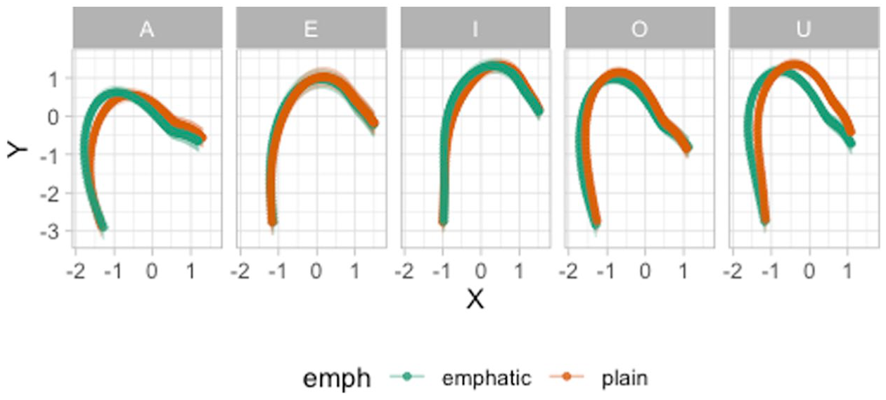
Predicted tongue contours with 95% CIs from an MGAM of Lebanese Arabic emphatic and plain coronal consonants.

In Figure 11, predictions have been calculated for individual speakers (see Article Notebook online, linked above, for the code). First, there is a good deal of individual variation: some speakers show a clear differentiation of the tongue shape in emphatic and plain consonants, while in other speakers the difference is less obvious. FAK produced emphatic and plain consonants with virtually the same tongue shape. Just to pick another example, BAR uvularized/velarized rather than pharyngealized the emphatic consonants followed by /I/, while BAY pharyngealized them. Plotting predictions of individual speakers can reveal idiosyncratic patterns which are not visible when plotting overall predictions.

Figure 11.

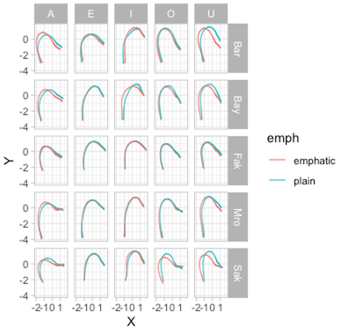
Predicted tongue contours with 95% CIs from an MGAM of Lebanese Arabic emphatic and plain coronal consonants split by speaker.

3 Multivariate functional principal component analysis

Principal Component Analysis (PCA) is a dimensionality reduction technique. For an introduction to PCA we recommend Kassambara (2017). Functional PCA (FPCA) is an extension of PCA: while classical PCA works by finding common variance in a set of variables (and by reducing the variables to Principal Components that explain that common variance), FPCA is a PCA applied to a functional representation of varying numerical variables (Gubian, 2024; Gubian et al., 2015, 2019; Ramsay & Silverman, 2005): a typical example is time-series data, with a variable changing over time. The trajectory of the time-varying variable is encoded into a function with a set of coefficients and the values of those coefficients are submitted to PCA. When more than one time-varying variable is needed, this is where Multivariate FPCA (MFPCA) comes in (Gubian, 2024).

MFPCA is an FPCA applied to two or more response variables. Note that the variable does not have to be time. The variation can be on any linear variable: in the case of DLC-tracked UTI data, the variation happens along the knot number. Look back at Figure 5: the two varying variables are the X and Y coordinates, which are varying along the DLC knots. As with MGAMs, it is these two varying trajectories that are submitted to MFPCA.

3.1 VC coarticulation

We will apply Multivariate Functional Principal Component Analysis (MFPCA) to the data introduced in Section 2.1. The following code has been adapted from Gubian (2024). The packages below are needed to run MFPCA (except landmarkregUtils, they are available on CRAN).

library(fda)

library(funData)

library(MFPCA)

# install.packages("remotes")

# remotes::install_github("uasolo/landmarkregUtils")

library(landmarkregUtils)

The format required to work through MFPCA is a “long” format with one column containing the coordinate labels (x or y coordinate) and another with the coordinate values. We can easily pivot the data with pivot_longer(). Note that we are using the z-scored coordinate values (X_z and Y_z). If you are unsure about the code in this section, it is always useful to inspect intermediate and final output in the pipe chains to familiarize yourself with the format of the input and resulting data.

dlc_voff_long <- dlc_voff_f |>

# Select relevant columns

dplyr::select(X_z, Y_z, frame_id, knot, vowel, c2_place, language, speaker) |>

# Pivot data to longer format. Saves coordinate labels to column `dim`

pivot_longer(c(X_z, Y_z), names_to = “dim”)

In the second step, we create a multiFunData object: this is a special type of list object, with the observations of the two coordinates (X_z and Y_z) as two matrices of dimension $N \times 22$ , where N is the number of tongue contours and 22 is for the 11 knots for each of the two coordinates (X and Y) returned by DLC. Three columns in the data are used to create the multiFunData object: one column with the id of each contour (in our data, frame_id), a time or series column (knot) and the column with the coordinate values (value).

curves_fun_2d <- lapply(

c(“X_z”, “Y_z”),

function(y) {

long2irregFunData(

dlc_voff_long |> filter(dim == {{y}}),

# Tongue contour ID

id = “frame_id”,

# Knot column

time = “knot”,

# X/Y coordinate values

value = “value”

) |>

as.funData()

}

) |>

multiFunData()

Once we have our multiFunData object, we can use the MFPCA() function to compute an MFPCA. Since the data has 11 knots for each dimension, the total number of univariate PCs that can be calculated is 11 (n_pc in the code below). The argument M is the number of univariate PCs times the number of dimensions, here 2 (X and Y).

# Maximum number of univarite PCs, here 11 knots

n_pc <- 11

# Number of multivariate functional PC, i.e. number of dimensions * n_pc

M <- 2 * n_pc

# Compute MFPCA

mfpca <- MFPCA(

curves_fun_2d,

M = M,

uniExpansions = list(list(type = “uFPCA”, npc = n_pc), list(type = “uFPCA”, npc = n_pc))

)

We can quickly calculate the relative proportion of explained variance of all the PCs with the following code. Note that higher order PCs tend to explain less and less variance (as it can be seen in the output of the following code). The first two PCs alone account for about 70% of the variance.

# Proportion of explained variance

(mfpca$values / sum(mfpca$values)) |> round(2)

[1] 0.49 0.20 0.18 0.04 0.03 0.02 0.01 0.01 0.00 0.00 0.00 0.00 0.00 0.00 0.00

[16] 0.00 0.00 0.00 0.00 0.00 0.00 0.00

The best way to assess the effect of the PCs on the shape of the tongue contours is to plot the predicted tongue contours based on a set of representative PC scores. To be able to plot the predicted contours, we need to calculate them from the MFPCA object. It is suggested to plot predicted curves at score intervals based on fractions of the scores’ standard deviation. This is what the following code does. For illustration, we focus on PC1 and PC2 only.

# Get the PC score SD

sd_fun <- sqrt(mfpca$values)

# PC curves to be plotted

pc_curves <- expand_grid(

# PC 1 and 2 only

PC = 1:2,

dim = 1:2,

# Set the SD fraction, from -1 SD to +1 SD, with increments of 0.25

sd_frac = seq(-1, 1, by = 0.25)

) |>

group_by(PC, dim, sd_frac) |>

# We can now calculate the predicted contour with funData2long1().

# reframe() is needed because the funData2long1() function returns a data frame

# that has more rows than the original.

reframe(

funData2long1(

mfpca$meanFunction[[dim]] +

sd_frac * sd_fun[PC] * mfpca$functions[[dim]][PC],

time = “knot”, value = “value”

)

) |>

# We relabel the dimensions

mutate(

dim = factor(dim, levels = c(2, 1), labels = c(ꞌY_zꞌ, ꞌX_zꞌ))

)

The created data frame pc_curves has the predicted values of the X and Y coordinates along the knots. This is the same structure as Figure 5, with the knot number on the x-axis and the coordinates on the y-axis. Of course, what we are after is the X/Y plot of the tongue contours, rather than the knot/coordinate plot as needed to fit an MFPCA. For the sake of clarity, we first plot the predicted curves for X and Y separately. Figure 12 shows these. The plot is composed of four panels: the top two are the predicted curves along knot number for the Y coordinates (based on PC1 score in the left panel and PC2 score in the right panel). Interpreting the effect of the PCs scores on the X and Y coordinates separately allows one to observe vertical (Y coordinate) and horizontal (X coordinate) differences in tongue position independently. However, note that the vectors of muscle contractions in the tongue are not simply along a vertical/horizontal axis, as mentioned in Section 1. Looking at a full tongue contour (in an X/Y coordinates plot) will generally prove to be more straightforward.

Figure 12.

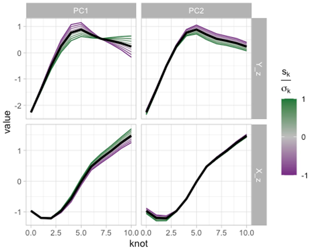
Predicted curves along knot number for X and Y coordinates, as obtained from an MFPCA.

To plot tongue contours in the X/Y coordinate system, we simply need to pivot the data to a wider format.

pc_curves_wide <- pc_curves |>

pivot_wider(names_from = dim)

Figure 13 plots the predicted contours based on the PC scores (specifically, fractions of the standard deviation of the PC scores). The x and y-axes correspond to the X and Y coordinates of the tongue contour, with the effect of PC1 score in the left panel and the effect of PC2 score in the right panel. A higher PC1 score (green lines in the left panel) suggests lowering of the tongue body/dorsum and raising of the tongue tip. Since the data contains velar and coronal consonants, we take this to be capturing the velar/coronal place of articulation. A higher PC2 score (green lines in the right panel) corresponds to an overall higher tongue position. Considering that the back/central vowels /a, o, u/ are included in this data set, we take PC2 to be related to the effect of vowel on the tongue shape at closure onset.

Figure 13.

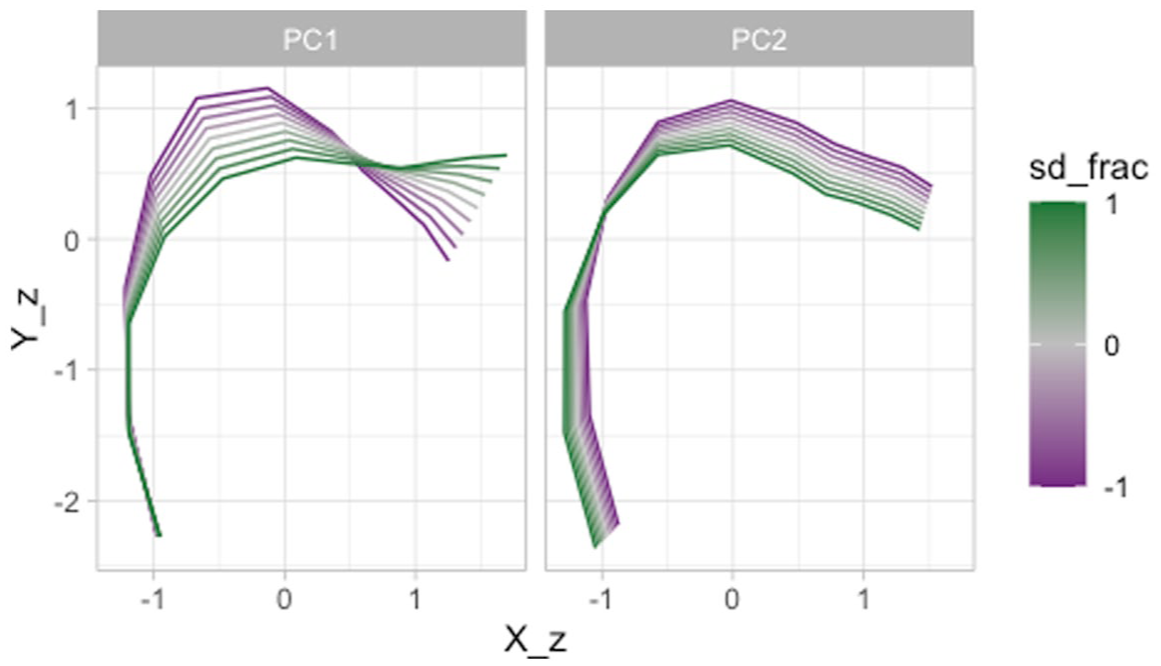
Predicted tongue contours as obtained from an MFPCA.

Given the patterns in Figure 13, we can expect to see differences in PC2 scores based on the vowel if there is VC coarticulation. We can obtain the PC scores (named sN where N is the PC order from 1 to 22) of each observation in the data with the following code.

pc_scores <- mfpca$scores |>

`colnames<-`(paste0("s", 1:M)) |>

as_tibble() |>

bind_cols(dlc_voff_long |> distinct(frame_id, vowel, c2_place, language))

Figure 14 plots PC scores by language (rows), consonant place (columns) and vowel (color). Both in Italian and Polish, we can observe a clear coarticulatory effect of /u/ on the production of coronal stops (and perhaps minor differences in /a/ vs. /o/). On the other hand, the effect of vowel in velar stops seems to be minimal, again in both languages. This is not entirely surprising, since while coronal stops allow for adjustments of (and coarticulatory effect on) the tongue body, velar stops do not since it is precisely the tongue body/dorsum that is raised to produce the velar closure.

Figure 14.

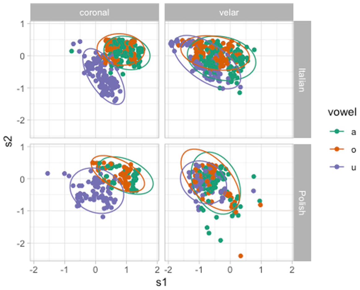
PC1/PC2 scores by language, consonant place of articulation and vowel.

Once one has established which patterns each PC is capturing, PC scores can be submitted to further statistical modeling, like for example regression models in which the PC scores are outcome variables and predictors are included to assess possible differences in PC scores, or in which the PC scores are predictors themselves. We illustrate an example regression model at the end of the following section for the Lebanese Arabic emphaticness data.

3.2 Emphaticness

In this section we will run an MFPCA analysis on the Lebanese Arabic data. Since the procedure is the same as in the previous section, the code will not be shown here, but can be viewed in the Article Notebook, available at https://stefanocoretta.github.io/mv_uti/index-preview.html.

Figure 15 illustrates the reconstructed tongue contours (taken from 35 ms before the CV boundary) in Lebanese Arabic, based on the MFPCA. PC1 captures the low-back/high-front diagonal movement. PC2, on the other hand, seems to be restricted to high/low movement at the back of the oral cavity. Emphatic consonants, if produced with a constricted pharynx (i.e., pharyngealized), should have a lower PC1. If on the other hand they are produced with a raised tongue dorsum (i.e., uvularized/velarized), they should have a lower PC2 (lower PC scores are in purple in Figure 15).

Figure 15.

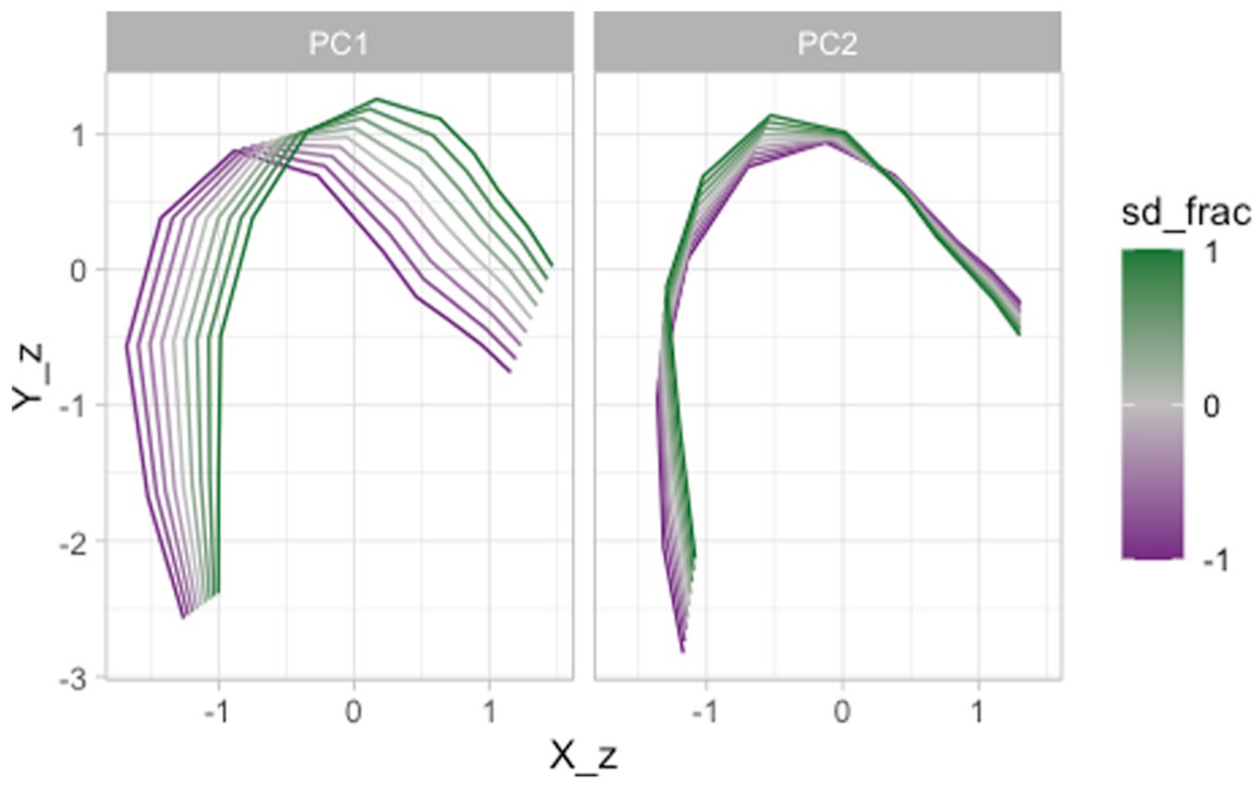
Predicted tongue contours of Lebanese Arabic coronal consonants as obtained from an MFPCA.

Figure 16 plots the PC scores for each vowel, emphaticness and speaker combination. Points are colored based on emphaticness: emphatic in green and plain in orange. This figure illustrates well how the PC scores can capture individual variation: some speakers show clear separation of emphatic and plain tokens, while others do not. In most cases, PC1 is doing the heavy lifting of distinguishing emphatic and plain: recall that PC1 captures the front-high/back-low diagonal; a low PC1 indicates tongue dorsum and root backing, in other words pharyngealization. Indeed, PC1 tends to be lower in emphatic tokens in several speakers, like BAR, BAY, MRO and SAK, especially with the vowels /A, O, U/. On the other hand, BAR’s emphatic and plain tokens for vowels /E, I/ do not show a PC1 difference, but rather a PC2 difference: PC2 captures tongue dorsum/body raising, hence indicating velarization. It is possible that in BAR’s productions of emphatic consonants followed by /E, I/ the distinction with plain is produced by uvularization/velarization, compared with the pharyngealization of emphatic consonants followed by /A, O, U/. Uvularization/velarization, rather than pharyngealization, in the /E, I/ contexts makes sense given that the tongue root has to be forward for the production of those vowels (see Sakr, 2025), Section 6.4 for more details).

Figure 16.

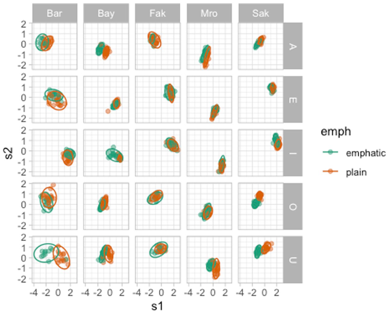
PC1 and PC2 scores by vowel, consonant type and speaker.

Figures 17 and 18 illustrate one way to plot the PC scores individually for PC1 and PC2. We won’t include here a full description of the plots, since they should be self-explanatory, but we flag to the reader that these type of plots can be helpful in illustrating specific patterns in PC1 or PC2 scores.

Figure 17.

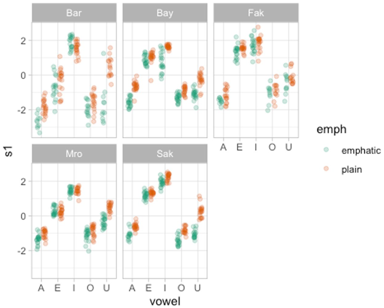
PC1 scores of emphatic and plain consonants by speaker and vowel.

Figure 18.

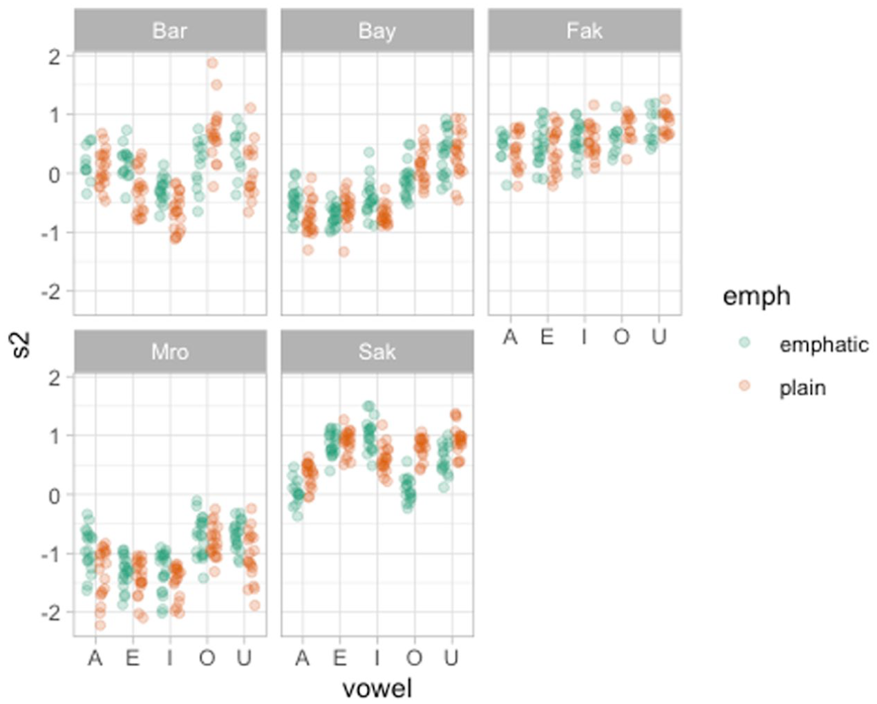
PC2 scores of emphatic and plain consonants by speaker and vowel.

Furthermore, it can be helpful to reconstruct the predicted tongue contours of specific contexts. For example, we might be interested in showing the average tongue contours for emphatic and plain consonants followed by each of the five vowels in the data. This is shown in Figure 19. To obtain the reconstructed contours, we first need to calculate mean PC scores for each vowel. This can be done through the following code. We recommend to inspect the pc_scores_mean object in R.

pc_scores_mean <- pc_scores |>

# Group by variables based on which we want to obtain mean values.

group_by(vowel, emph) |>

# Sumarise data to obtain means

summarise(

s1 = mean(s1),

s2 = mean(s2),

.groups = “drop”

) |>

# Add “dimensions”, i.e. X and Y coordinates

mutate(

dim = list(c(1, 2))

) |>

# Unnes the dim column

unnest(dim)

The following code calculates the reconstructed tongue contours based on both PC1 and PC2. One could also calculate the reconstructed contours at fractions of the standard deviation of the scores if one wished so, like it was done above.

pc_curves_2 <- pc_scores_mean |>

group_by(dim, vowel, emph) |>

# We can now calculate the predicted contour with funData2long1().

# reframe() is needed because the funData2long1() function returns a data frame

# that has more rows than the original.

reframe(

funData2long1(

mfpca$meanFunction[[dim]] +

# We add PC1

s1 * mfpca$functions[[dim]][1] +

# and we add PC2 as well

s2 * mfpca$functions[[dim]][2],

time = “knot”, value = “value”

)

) |>

# We relabel the dimensions

mutate(

dim = factor(dim, levels = c(2,1), labels = c(ꞌY_zꞌ, ꞌX_zꞌ))

) |>

pivot_wider(names_from = dim, values_from = value)

Finally, Figure 19 plots the reconstructed contours. Based on this figure, we do find pharyngealization in emphatic consonants followed by /A, O, U/ on average, while pharyngealization is absent in the context of /E, I/.

Figure 19.

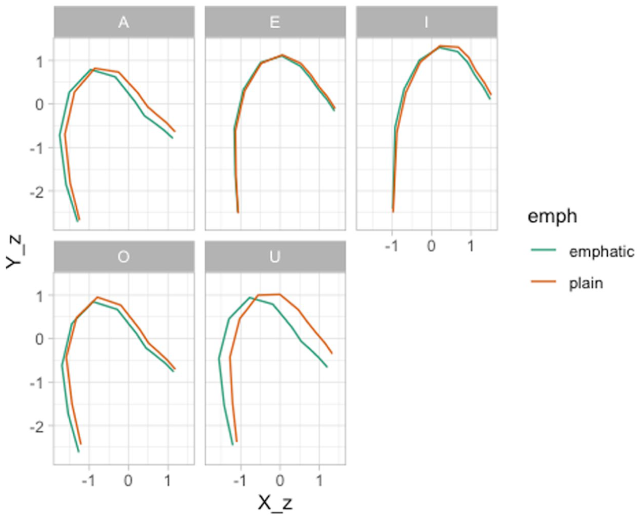
Reconstructed tongue contours based on PC1/PC2.

To illustrate how the PC scores can be further modeled using regressions, we fitted a Bayesian Gaussian regression model using brms (Bürkner, 2017, frequentist methods are of course also possible) with the PC1 score as the outcome, emphaticness (emphatic vs. plain) and vowel (A, E, I, O, U) and their interaction as predictors. We also included by-participant varying intercepts and varying slopes for the emphaticness/vowel interaction. Both emphaticness and vowel were coded using sum contrasts. This is the R formula we used: PC1 ~ emph_fac * vowel_fac + (emph_fac * vowel_fac—participant). We used the default priors as set by brms. Since a full introduction to regression modeling and Bayesian inference is beyond the scope of this paper, we refer the readers to the many resources now available. See the online version of the manuscript for the full code of the Bayesian analysis of PC1: https://stefanocoretta.github.io/mv_uti/.

Figure 20 shows the posterior distributions of the expected PC1 scores for emphatic and plain consonants followed by each of the vowels, based on the Bayesian regression model. A lower PC1 score suggests pharyngealization as established above. It can be observed that emphatic consonants have a lower PC1 score compared with plain consonants, across all vowels, albeit with different magnitudes in different vowels. Overall, the model suggests that the PC1 score of emphatic consonants is on average 0.04 to 0.88 units lower than plain consonants, at 95% confidence (mean effect = −0.48, SE = 0.22, 95% CrI [−0.88, −0.04], 80% CrI [−0.7, −0.28], 70% CrI [−0.65, −0.32]).

Figure 20.

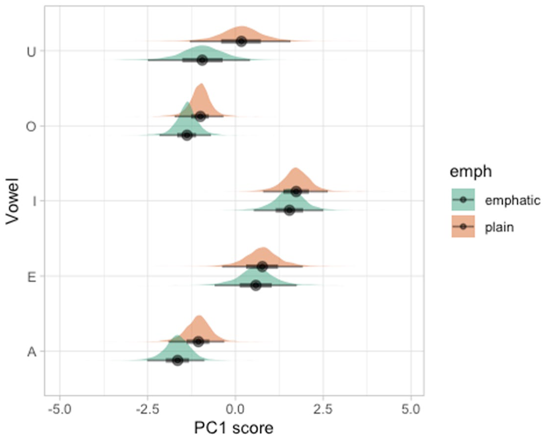
Posterior distributions of expected PC1 scores for emphatic and plain consonants, followed by different vowels, from a Bayesian regression model.

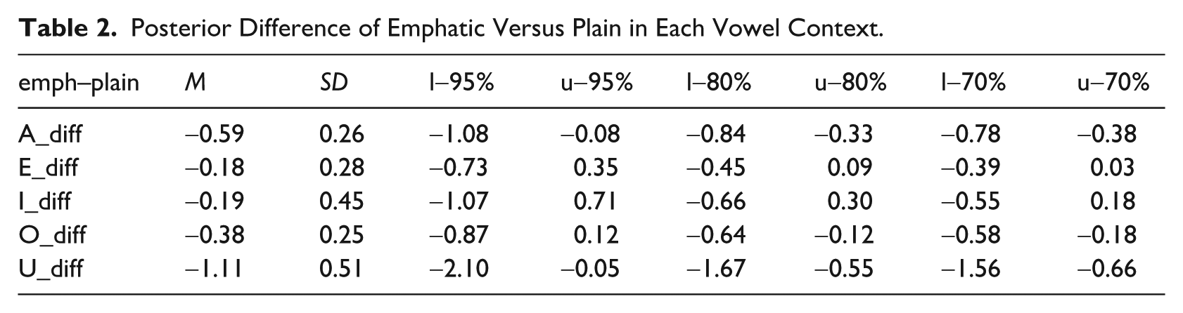
Table 2 shows the mean, standard deviation and 95-80-65% CrIs of the posterior difference between emphatic and plain consonants for each vowel. The CrIs indicate a robustly lower PC1 for /A, U/. For the other vowels, both a lower or slightly higher PC1 are possible and, if a difference is present at all, it would be of a lower magnitude than that in the /A, U/ context. At 80% confidence, emphatic consonants also show a lower PC1 when followed by /O/. In sum, while we can argue for a lower PC1 in the /A, U/ and possibly /O/ contexts (and hence, pharyngealization in emphatic consonants followed by these vowels), the results are more uncertain regarding /E, I/.

Table 2.

Posterior Difference of Emphatic Versus Plain in Each Vowel Context.

emph–plain	M	SD	l-95%	u-95%	l-80%	u-80%	l-70%	u-70%
A_diff	-0.59	0.26	-1.08	-0.08	-0.84	-0.33	-0.78	-0.38
E_diff	-0.18	0.28	-0.73	0.35	-0.45	0.09	-0.39	0.03
I_diff	-0.19	0.45	-1.07	0.71	-0.66	0.30	-0.55	0.18
O_diff	-0.38	0.25	-0.87	0.12	-0.64	-0.12	-0.58	-0.18
U_diff	-1.11	0.51	-2.10	-0.05	-1.67	-0.55	-1.56	-0.66

4 Advantages and disadvantages

Both Multivariate GAMs and FPCA are a useful way to model DLC-tracked ultrasound tongue imaging data. However, each possesses advantages and disadvantages.

Multivariate GAMs can model tongue contours in specific contexts and combinations thereof, like different vowels, consonant, prosodic contexts and so on. The rather complex model structure required to fit multivariate GAMs to tongue data comes at a computational cost and an interpretative cost. Computationally, multivariate GAMs can take hours to estimate even the most simple models. Interpretationally, comparing different tongue contours quantitatively based on the output of a multivariate GAM is non-trivial, given that the tongue contour is in fact a curve reconstructed from the smooths of the X and Y coordinates along knot (in other words, the model does not model tongue contours directly). Moreover, in the specific implementation of multivariate GAMs employed by mgcv, there is no straightforward way to use traditional methods to assess (frequentist) statistical significance. From a practical point of view, a multivariate GAM ends up being a mathematically complex way of obtaining a sort of average tongue contour. A further constraint is that mgcv offers only a multivariate Gaussian distribution, which might not always be an appropriate distribution (despite being a neutral assumption in the sense that it is appropriate when one is interested only in estimating a mean and standard deviation, see McElreath, 2020, p 75). We recommend users to check model assumptions with gam.check() from the mgcv package.

Multivariate FPCA, on the other hand, is computationally efficient (when factoring out time for further analyses, like in the case above where we fitted a regression model to the PC1 scores). Even with very large data sets, the computation of Principal Components is relatively quick. Moreover, the obtained PCs can be interpreted straightforwardly by plotting the effect of changing the PC score on the reconstructed tongue contour (as we did for example in Figure 13). One possible disadvantage of multivariate FPCA is that it is usually not known what type of variation each obtained PC captures. This is illustrated in the two case studies in Section 3. In the VC coarticulation data, PC1 corresponded to the coronal/velar difference in consonants, while PC2 to the difference in vowel. In the emphaticness data, PC1 captured the low-back/high-front diagonal movement, while PC2 to the high/low movement at the back of the oral cavity. In other words: until one has run the MFPCA, one cannot know which PC will correspond to which axis of differences, and whether the PCs will capture relevant differences at all. It can happen that the variation one is after is so minimal relative to other, more substantial cases of variation, that it will not be captured by the MFPCA at all. It is possible that qualitatively homogeneous data sets might return PCs that have the same or very similar interpretations. This has not been systematically tested, perhaps with the exception of simple PCA run on vowel formant data, which suggests that the first two PCs capture the two diagonals (Faber & Di Paolo, 1995; Hoole, 1999; Strycharczuk et al., 2021, 2025), which make sense in light of the tongue position and shape model expounded by Honda (1996). Another advantage of MFPCA is that, provided that the PCs have captured relevant characteristics, the PCs can be submitted to further modeling using regression with the inclusion of relevant predictors (like different categorical variables of interest) as we have illustrated in the previous section.

Note that a viable, but theoretically less robust, alternative is to model the data with the coordinates values as the outcome and the type of coordinate (X vs. Y) as a predictor, as done for example in Wieling et al. (2016) and Gubian (2025) (this approach models the X and Y coordinates as completely independent, while an MVGAM also estimates residual correlations between the two, which is a desired, although not deal-breaking, property).

Based on the advantages and disadvantages of each of multivariate GAMs and FPCA, we suggest to researchers to use MFPCA as the preferred and default approach to analyze DLC-tracked tongue contour data and to resort to multivariate GAMs if MFPCA fails to capture relevant variation.

5 Conclusion

This tutorial demonstrates two methods for analyzing tongue contour data derived from DeepLabCut: multivariate generalized additive models (MGAMs) and multivariate functional principal component analysis (MFPCA). We offer detailed, annotated analyses of two example datasets, focusing on vowel-to-consonant coarticulation in Italian and Polish, and emphatic consonants in Lebanese Arabic. All associated materials, including datasets and code, are accessible through the tutorial’s research compendium at https://github.com/stefanocoretta/mv_uti. In closing, we evaluated the strengths and limitations of each method and advise adopting MFPCA as the preferred initial modeling strategy for tongue contour data.

Footnotes

Funding

The authors received no financial support for the research, authorship, and/or publication of this article.

ORCID iDs

Stefano Coretta

Georges Sakr

Data availability statement

All the materials (including data and code) are available in the research compendium of the tutorial at https://github.com/stefanocoretta/mv_uti. An online version of the manuscript is available at .

Notes

References

Alorifi

F. S.

(2008). Automatic identification of Arabic dialects using hidden Markov models [PhD thesis, University of Pittsburgh, Pittsburgh, PA].

Al-Tamimi

Heselwood

(2011). Nasoendoscopic, videofluoroscopic and acoustic study of plain and emphatic coronals in Jordanian Arabic. In Heselwood

Hassan

Z. M.

(Eds.), Instrumental studies in Arabic phonetics (Vol. 319, pp. 165–191). John Benjamins.

Al-Tamimi

(2017). Revisiting acoustic correlates of pharyngealization in Jordanian and Moroccan Arabic: Implications for formal representations. Laboratory Phonology: Journal of the Association for Laboratory Phonology, 8(1), 28. https://doi.org/10.5334/labphon.19

Articulate Instruments Ldt. (2011). Articulate assistant advanced user guide. Version 2.16.

Bin-Muqbil

M. S.

(2006). Phonetic and phonological aspects of Arabic emphatics and gutturals. The University of Wisconsin-Madison.

Bürkner

P.-C.

(2017). Brms: An r package for Bayesian multilevel models using stan. Journal of Statistical Software, 80(1), 1–28. https://doi.org/10.18637/jss.v080.i01

Chen

Lin

(2011). Analysing tongue shape and movement in vowel production using SS-ANOVA in ultrasound imaging. In Proceedings of International Congress of Phonetic Sciences (ICPhS), International Phonetic Association (pp. 124–127). University of Victoria.

Coretta

(2018a). An exploratory study of the voicing effect in Italian and Polish [Data V1.0.0]. https://doi.org/10.17605/OSF.IO/8ZHKU

Coretta

(2018b). Using Generalised Additive Models (GAM) with polar coordinates for assessing tongue contours. https://stefanocoretta.github.io/rticulate/articles/polar-gams.html

10.

Coretta

(2019). Assessing mid-saggital tongue contours in polar coordinates using Generalised Additive (Mixed) Models. https://doi.org/10.31219/osf.io/q6vzb

11.

Coretta

(2020a). Longer vowel duration correlates with greater tongue root advancement at vowel offset: Acoustic and articulatory data from Italian and Polish. The Journal of the Acoustical Society of America, 147, 245–259. https://doi.org/10.1121/10.0000556

12.

Coretta

(2020b). Vowel duration and consonant voicing: A production study [PhD thesis, University of Manchester, Manchester].

13.

Davidson

(2006). Comparing tongue shapes from ultrasound imaging using smoothing spline analysis of variance. The Journal of the Acoustical Society of America, 120(1), 407–415. https://doi.org/10.1121/1.2205133

14.

Elhij’a

D. A.

(2012). Facebook written Levantine vernacular languages. Levantine Review, 1(1), 68–105. https://doaj.org/article/6698290a36c244f783a59ba49617e821

15.

El-Khaissi

(2015). The Romanisation of Arabic: A comparative analysis of Romanised spoken Arabic and Romanised modern standard Arabic [PhD thesis, La Trobe University, Melbourne, VIC, Australia].

16.

Epstein

M. A.

Stone

(2005). The tongue stops here: Ultrasound imaging of the palate. The Journal of the Acoustical Society of America, 118(4), 2128–2131. https://doi.org/10.1121/1.2031977

17.

Faber

Di Paolo

(1995). The discriminability of nearly merged sounds. Language Variation and Change, 7(1), 35–78. https://doi.org/10.1017/S0954394500000892

18.

Ghazeli

(1977). Back consonants and backing coarticulation in Arabic [PhD thesis, University Texas at Austin, Austin, TX].

19.

Gubian

(2024). Workshop on functional PCA for phonetics and prosody. https://github.com/uasolo/FPCA-phonetics-workshop

20.

Gubian

(2025). Analysis of uni- and multi-dimensional contours with GAMs and functional PCA: An application to ultrasound tongue imaging [Version 1.0.0]. https://uasolo.github.io/UTI-GAM-FPCA/

21.

Gubian

Pastätter

Pouplier

(2019). Zooming in on Spatiotemporal v-to-c Coarticulation with Functional PCA. Proceedings of Interspeech, 2019, 889–893. https://doi.org/10.21437/Interspeech.2019-2143

22.

Gubian

Torreira

Boves

(2015). Using functional data analysis for investigating multidimensional dynamic phonetic contrasts. Journal of Phonetics, 49(March), 16–40. https://doi.org/10.1016/j.wocn.2014.10.001

23.

Happ

Greven

(2018). Multivariate functional principal component analysis for data observed on different (dimensional) domains. Journal of the American Statistical Association, 113, 649–659. https://doi.org/10.1080/01621459.2016.1273115

24.

Happ-Kurz

(2022). MFPCA: Multivariate Functional Principal Component Analysis for data observed on different dimensional domains. https://github.com/ClaraHapp/MFPCA

25.

Hastie

Tibshirani

(1986). Generalized additive models. Statistical Science, 1(3), 297–310. https://doi.org/10.1201/9780203753781-6

26.

Honda

(1996). Organization of tongue articulation for vowels. Journal of Phonetics, 24(1), 39–52. https://doi.org/10.1006/jpho.1996.0004

27.

Hoole

(1999). On the lingual organization of the German vowel system. The Journal of the Acoustical Society of America, 106(2), 1020–1032. https://doi.org/10.1121/1.428053

28.

Kassambara

(2017). Practical guide to principal component methods in r. STHDA.

29.

Khattab

Al-Tamimi

Heselwood

(2006). Acoustic and auditory differences in the /t/-/ṭ/ opposition in male and female speakers of Jordanian Arabic. In Boudelaa

(Ed.), Perspectives on Arabic Linguistics: Papers from the Annual Symposium on Arabic Linguistics (Vol. XVI., pp. 131–160). John Benjamins Publishing Company.

30.

Lian

(2022). Language, ideology and sociopolitical change in the Arabic-speaking world: A study of the discourse of Arabic language academies / Chaoqun Lian. Edinburgh University Press. https://doi.org/10.1515/9781474449960

31.

Lulich

S. M.

Berkson

K. H.

de Jong

(2018). Acquiring and visualizing 3d/4d ultrasound recordings of tongue motion. Journal of Phonetics, 71, 410–424. https://doi.org/10.1016/j.wocn.2018.10.001

32.

Mathis

Mamidanna

Cury

K. M.

Abe

Murthy

V. N.

Mathis

M. W.

Bethge

(2018). DeepLabCut: Markerless pose estimation of user-defined body parts with deep learning. Nature Neuroscience, 21(9), 1281–1289. https://doi.org/10.1038/s41593-018-0209-y

33.

McElreath

(2020). Statistical rethinking: A Bayesian course with examples in R and stan [CRC Texts in Statistical Science Series] (2nd ed.). CRC Press.

34.

Nasr

R. T.

(1959). Velarization in Lebanese Arabic. Phonetica, 3(4), 203–209. https://doi.org/10.1159/000257920

35.

Obrecht

D. H.

(1968). Effects of the second formant on the perception of velarization consonants in Arabic [Reprint 2017. Janua linguarum; 39, Ser. Practica]. De Gruyter Mouton.

36.

Pedersen

E. J.

Miller

D. L.

Simpson

G. L.

Ross

(2019). Hierarchical Generalized Additive Models in Ecology: An Introduction with Mgcv. PeerJ, 7, Article e6876. https://doi.org/10.7717/peerj.6876

37.

Pettersson

Wood

(1987). Vowel reduction in Bulgarian and its implications for theories of vowel production: A review of the problem. Folia Linguistica, 21(2–4), 261–280. https://doi.org/10.1515/flin.1987.21.2-4.261

38.

Ramsay

J. O.

Silverman

B. W.

(2005). Functional data analysis [Springer Series in Statistics]. Springer. https://doi.org/10.1007/b98888

39.

Sakr

(2019). A laboratory phonology investigation into the vocalic inventory of Lebanese [Master’s thesis, University of Edinburgh, Edinburgh].

40.

Sakr

(2023). On the acoustics of emphasis in Central Mount Lebanon Lebanese. Journal of Semitic Studies, 69(1), 601–642. https://doi.org/10.1093/jss/fgad024

41.

Sakr

(2025). The phonetics of emphasis in Central Mount Lebanon Lebanese: Acoustics, perception, articulation [PhD thesis, University of Edinburgh, Edinburgh].

42.

Scobbie

J. M.

Lawson

Cowen

Cleland

Wrench

A. A.

(2011). A Common co-ordinate system for mid-sagittal articulatory measurement. https://eresearch.qmu.ac.uk/items/3636d78a-a69f-4b50-a746-e293add7d6bc

43.

Shaaban

Ghaith

(1999). Lebanon’s language-in-education policies: From bilingualism to trilingualism. Language Problems and Language Planning, 23(1), 1–16.

44.

Sóskuthy

(2021a). Evaluating Generalised Additive Mixed Modelling Strategies for Dynamic Speech Analysis. Journal of Phonetics, 84, 101017. https://doi.org/10.1016/j.wocn.2020.101017

45.

Sóskuthy

(2021b). Generalised Additive Mixed Models for dynamic analysis in linguistics: A practical introduction. https://doi.org/10.48550/arXiv.1703.05339

46.

Stone

(2005). A guide to analysing tongue motion from ultrasound images. Clinical Linguistics & Phonetics, 19(6–7), 455–501. https://doi.org/10.1080/02699200500113558

47.

Strycharczuk

Ćavar

Coretta

(2021). Distance vs time. Acoustic and articulatory consequences of reduced vowel duration in Polish. The Journal of the Acoustical Society of America, 150(1), 592–607. https://doi.org/10.1121/10.0005585

48.

Strycharczuk

Kirkham

Gorman

Nagamine

(2025). Dimensionality reduction in lingual articulation of vowels: Evidence from lax vowels in Northern Anglo-English. Language and Speech, 68(3), 689–721. https://doi.org/10.1177/00238309251320581

49.

Sullivan

(2017). Writing Arabizi: Orthographic variation in Romanized Lebanese Arabic on Twitter [PhD thesis, The University of Texas at Austin, Austin, TX].

50.

Watson

J. C. E.

(2002). The phonology and morphology of Arabic [Phonology of the world’s languages]. Oxford University Press.

51.

Wieling

(2018). Analyzing dynamic phonetic data using generalized additive mixed modeling: A tutorial focusing on articulatory differences between L1 and L2 speakers of English. Journal of Phonetics, 70, 86–116. https://doi.org/10.1016/j.wocn.2018.03.002

52.

Wieling

Tomaschek

Arnold

Tiede

Bröker

Thiele

Wood

S. N.

Baayen

R. H.

(2016). Investigating dialectal differences using articulography. Journal of Phonetics, 59(November), 122–143. https://doi.org/10.1016/j.wocn.2016.09.004

53.

Wood

(2006). Generalized Additive Models: An introduction with r. CRC Press.

54.

Wrench

(2024). The compartmental tongue. Journal of Speech, Language, and Hearing Research, 67(10S), 3887–3913. https://doi.org/10.1044/2024_jslhr-23-00125

55.

Wrench

Balch-Tomes

(2022). Beyond the edge: Markerless pose estimation of speech articulators from ultrasound and camera images using DeepLabCut. Sensors, 22(3), 1133. https://doi.org/10.3390/s22031133

56.

Zawaydeh

B. A.

(1999). The phonetics and phonology of gutturals in Arabic [PhD thesis, Indiana University, Bloomington, IN].

57.

Zeroual

Esling

J. H.

Hoole

(2011). EMA, endoscopic, ultrasound and acoustic study of two secondary articulations in Moroccan Arabic. In Heselwood

Hassan

Z. M.

(Eds.), Instrumental studies in Arabic phonetics (Vol. 319, pp. 277–298). John Benjamins.

Multivariate Analyses of Tongue Contours from Ultrasound Tongue Imaging

Abstract

Keywords

1 Introduction

2 Multivariate generalized additive models

2.1 VC coarticulation

2.2 Emphaticness

3 Multivariate functional principal component analysis

3.1 VC coarticulation

3.2 Emphaticness

4 Advantages and disadvantages

5 Conclusion

Footnotes

Funding

ORCID iDs

Data availability statement

Notes

References