Guidelines on statistics for researchers using laboratory animals: the essentials

Abstract

There is growing concern that the omnipresence of flawed statistics and the deficient reproducibility that arises therefrom results in an unethical waste of animals in research. The present review aims at providing guidelines in biostatistics for researchers, based on observed frequent mistakes, misuses and misconceptions as well as on the specificities of animal experimentation. Twelve recommendations are formulated that cover sampling, sample size optimisation, choice of statistical tests, understanding p-values and reporting results. The objective is to expose important statistical issues that one should consider for the correct design, execution and reporting of experiments.

Statistics is the science of rigorously quantifying uncertainty, and applying it to life sciences (i.e. biostatistics) has become indispensable due to the capriciousness of biological readouts. In animal research, flawless biostatistics is essential for interpreting and reproducing results and thus avoiding the unnecessary and unethical use of animals. Despite this, there is a well-documented universal misunderstanding and misuse of biostatistics, which can have critical consequences on the validity of the research.^1,2 Mistakes in experimental design,^2–4 interpretation of p-values,^5,6 statistical analysis,^7–9 and presentation,^10,11 can result in devastating ethical and financial costs and low success rates of subsequent clinical trials or technology development. The present article aims to introduce good practices into biostatistics in research employing laboratory animals. I will expose pitfalls and mistakes frequently encountered, followed by viable recommendations.

Scope and limitations

The review is addressed mainly to life scientists who are not familiar with the fundamental concepts of statistics but who need to use biostatistics in their research activity. Nevertheless, life scientists with a more advanced command of statistics could use the present article as a ‘refresher course’. The review focuses on statistics and will only touch upon ethical issues. It will begin with a very brief introduction that reviews the important concepts in biostatistics and is then divided into sections that recapitulate the three arms of quantitative experiments, namely design, analysis and reporting. Each section is sub-divided into a series of recommendations (Figure 1). Nevertheless, the author is aware that concepts addressed in distinct sections and subsections are interconnected. Furthermore, although prepared with the objective of guiding researchers involved in animal research, the concepts exposed herein are fully generalisable to other scientific fields such as in-vitro or clinical studies. Finally, the entire world of biostatistics cannot be covered in a single review; consequently, this review will focus on a selection of topics deemed more relevant for a journal about animal research. Therefore, some readers from specific domains or with precise expectancies (for example in statistics not based on hypothesis testing), might find this thematic selection and the angle by which these issues are covered hereafter somewhat partial.

Figure 1.

Overview of the recommendations suggested in the present article.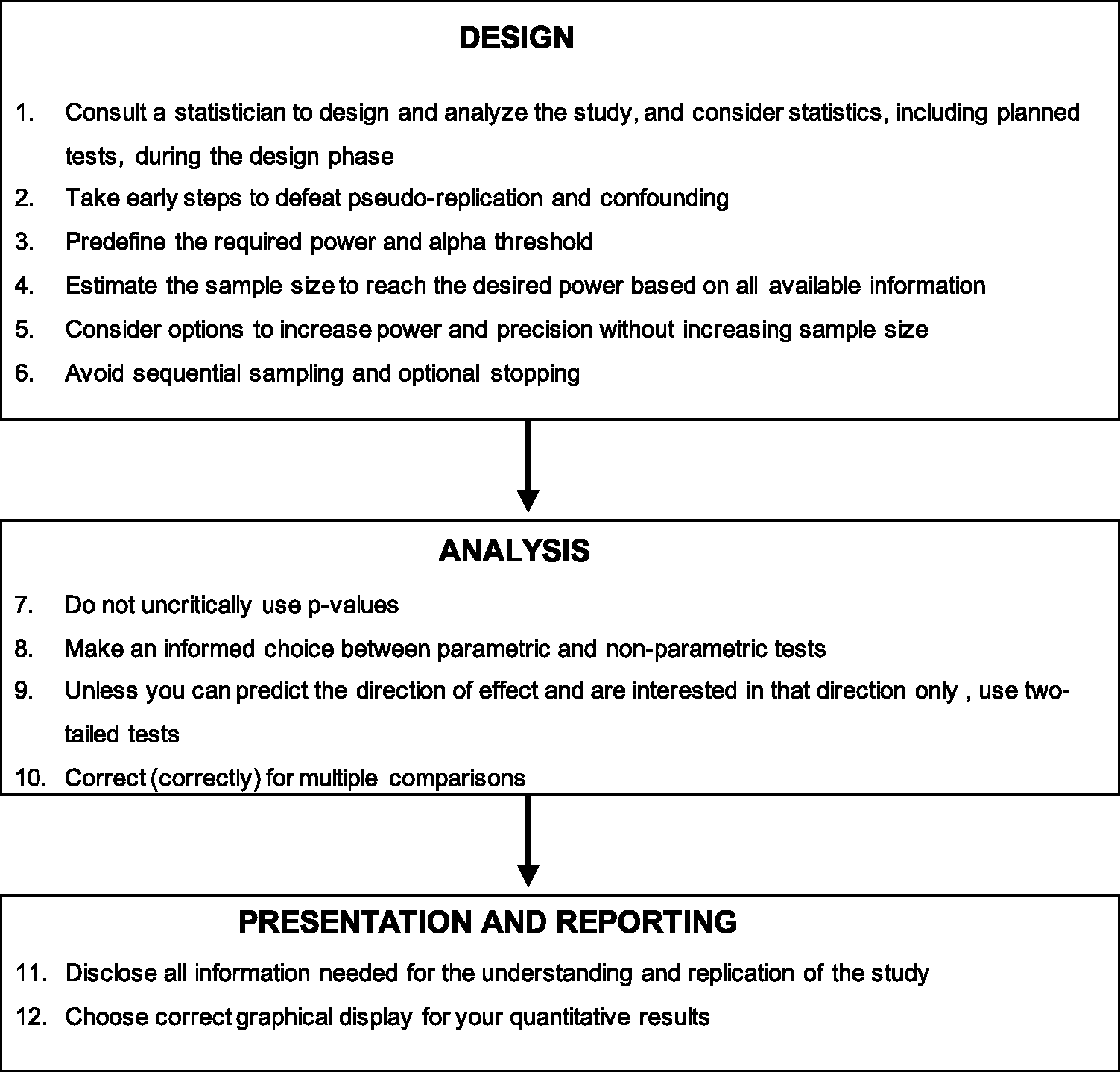

Hypothesis testing

The following paragraph serves as a very concise outline on the specific domain of hypothesis testing and gives the backbone of the notions and terminology exposed hereafter.

Life scientists study populations, a term defined as the total set of observations that can be made. However, populations are often (if not always) inaccessible; therefore, scientists rely on small subsets of observations named samples. Experimental units are the smallest entities that can be assigned to a treatment and, therefore, at the same time are the true biological replicates that can be randomised and used to form a sample of independent observations. This notion of independence is defined by the fact that the value of one experimental unit does not affect the value of another. On the other hand, sampling units are the smallest entities that will be measured or observed. When multiple sampling units are taken from each experimental unit, they are called technical replicates.

Populations of interest are characterised by their properties, named parameters, whereas the estimates of these parameters in samples are eponymously called statistics. Researchers may want to simply describe the properties of the samples through so-called descriptive statistics or, conversely, try to reach conclusions about population parameters from the samples using inferential statistics. Adequate experimental designs ensure good internal validity (i.e. validity of the method that enables the experiment to draw inferences) and external validity (i.e. generalisability) of the study, which can both be threatened by many flaws in the research protocol. The important ones are covered in the present review. Investigators often study relationships between so called independent variables (the values of which are ‘controlled’ by the experimenter, such as sex or treatment) and dependent variables (variables the investigator quantifies). To avoid confusion between different uses and meanings of the term “independence”, the words input and output variables are preferred throughout the text. Input variables are called factors when categorical (e.g. groups, such as sex) and the different values they take are called levels (e.g. male or female).

The idea that scientific questions may have clear-cut answers is almost invariably irrelevant in the life sciences because observations are naturally fickle, even when collected from the same individual, but also due to variability that arises from measurements. The purpose of statistical tests is to extract the necessary information by removing the noisy background to attempt to make decisions about populations. The most frequent approach is null hypothesis significance testing (NHST), which is measured using a p-value. Despite their great diversity, statistical tests generally proceed in a similar series of steps: 1. based on the biological question, a so-called null hypothesis (H₀) is formulated, which theorises the absence of effect, relationship or difference; 2. data are collected and the effect, difference or relationship observed is converted into a statistic (usually named with a single letter or symbol depending on the test); 3. the p-value is calculated, which corresponds to the probability of obtaining this statistic or a larger one if H₀ is true; and, finally, 4. a biological conclusion is drawn, usually based on a comparison between p and an alpha threshold (usually set at 5% in life sciences). This classical approach of NHST is called the Neyman-Pearson approach.

Depending on the question asked and hypothesis formulated, statistical tests belong to categories that differ in the precise way they work. Throughout the article, we will often refer to notions and thinking that belong to so-called location tests (such as Student’s t-test), which make inferences about central tendency (i.e. mean, median) of the population. This relative focus is justified by the prevalence of these tests in animal research, which makes their terminology familiar to researchers. However, other families of tests exist, such as variance tests (e.g. Levene’s test), proportion tests (e.g. Chi ² test), association tests (e.g. Pearson’s and Spearman’s correlation) or distribution tests (e.g. Shapiro-Wilk test or Kolmogorov-Smirnov test), and will be mentioned periodically.

Importantly, great care must be given not to confuse terms and notions used in statistics with their counterparts in common language. For example, when comparing blood pressure between mice and rats, the statistical population refers to the values of the blood pressure not the species, which are obviously different biological populations.

Statistical design

Recommendation 1: Consult a statistician to design and analyse the study, and consider statistics, including planned tests, during the design phase

In 1938, Ronald Fisher, one of the founders of modern statistics, stated that ‘to call in the statistician after the experiment is done may be no more than asking him to perform a post-mortem examination: he may be able to say what the experiment died of’. ¹² Following on from this, in their landmark article published in 2004 entitled Guidelines for reporting statistics in journals published by the American Physiological Society, Curran-Everett and Benos introduced nine guidelines for designing and reporting quantitative results in physiology, and suggested that researchers should consult a statistician if in doubt when planning the study. ¹³ The attention given to statistics at a very early stage of the research project is salutary since flaws in design are often irreversible and require a completely new experiment. Among others, early important considerations include the type of variables to be measured, the unpaired or paired (repeated measures) nature of the observations, the number of experimental groups, the conditions of animal housing or the sex to be used. A professional statistician will help define such important considerations since accumulating evidence suggests that most researchers are not sufficiently proficient in experimental design and biostatistics to do it alone. ¹⁴ These decisions determine the nature of future statistical analyses to be performed and therefore the subsequent power and sample size calculations (see Recommendations 3, 4 and 5). Figure 2 illustrates this point by showing how input and output variables influence the subsequent statistical tests.

Figure 2.

Influence of the nature of the variables on the subsequent statistical tests. Grey boxes outlined in bold are expanded in tables indicated by arrows to illustrate the hidden multiple possibilities and choices that exist within each box. The list of tests is not exhaustive.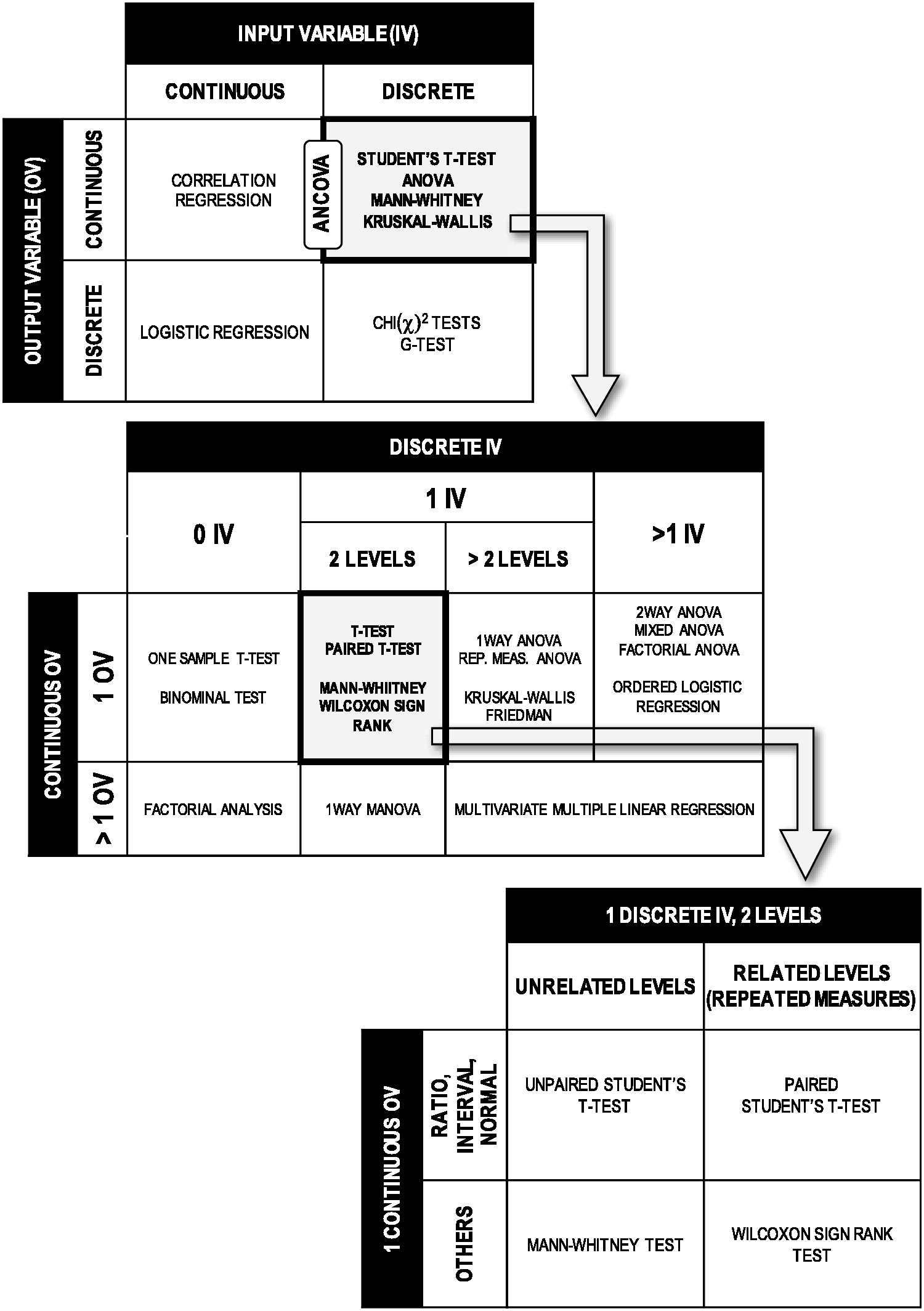

For example, the collection of a continuous variables (e.g. tumor size or plasma cytokine concentration) allows the use of a parametric test (see Recommendation 8) for data analysis, but such tests are very sensitive to extreme individual values (outliers). In this example, the investigator must therefore consider very early what policy to implement regarding outlier exclusion and the alternative possibility of collecting categorical variables (e.g. disease score or nature of cancerous organ) instead. These early decisions will constitute the backbone on which the entire design is built. It is recommended to systematically review the literature or perform a pilot study to get valuable information about the variables of interest.

A particular point to note here is the selection of the sex of the animals in the experimental design since males and females may display divergent biological readouts. Experimental designs usually incorporate only one sex, males in the majority of cases, in an attempt to reduce the total variability. ¹⁵ It should not be ignored that this selection bias may impede the validity of the study. ¹⁶ This point has been well demonstrated in recent studies on preclinical models of chronic pain for which years of mechanistic research conducted on male rodents turned out to be untrue in females.^17,18 The inclusion of both sexes can be made through specific designs such as factorial designs. This allows the estimation of treatment effect, sex effect, and the effect due to the interaction of both. ¹⁹

Recommendation 2: Take early steps to defeat pseudo-replication and confounding

Pseudo-replication, as coined by Hurlbert, is defined as ‘the use of inferential statistics to test for treatment effects with data from experiments where either treatments are not replicated (though samples may be) or replicates are not statistically independent’. ²⁰ On the other hand, confounding refers to a situation in which the association or effect between the variables is distorted by the existence of (at least) another variable. Although not synonymous, both issues may arise from insufficiently defining the exact structure of the experiment, i.e. the identification, selection, and definition of variables and levels, as well as the rules by which the levels will be allocated to the experimental units.

Pseudoreplication may occur when the investigator fails to distinguish experimental and sampling units. In view of the definitions presented in the Introduction, it appears that, although experimental and sampling units may be the same objects, in many designs they will be distinct. For example, the collection of a series of biopsies as technical replicates from each animal in an experiment is an example of multiple sampling units for each experimental unit. It implies that the final sample size (basis of the statistical analysis) is the number of animals, not the number of biopsies. Wrongly considering sampling units as independent experimental observations artificially inflates sample sizes, violates the principle of independence and results in an invalid analysis. Greater care must therefore be taken to correctly define and identify experimental units during the design, in other words to identify which objects will be the independent observations in the future statistical analysis.

In the above-mentioned example, the identification of experimental (rats) and sampling (biopsies) units was intuitive, but the task may require more careful attention for some designs. A frequent scenario unfolds when animals housed in the same cage are not independent because housing cage influences the output variable. Indeed, some biological readouts such as food consumption, ²¹ gut microbiota,^22,23 emotionality, ²⁴ or eye pathology due to light intensity, ²⁵ are influenced by the specific housing conditions of the cage or by animal interactions within the cages. Here, if all animals within the same cages are exposed to the same treatment, animals are not independent observations, since the actual design structure is that cages are the actual experimental units (they are randomised to the treatment) and the animals are the sampling units.

In the above example, “cage” is not an input variable of primary interest but even so may influence the value of the output variable. It is called a cofactor because this variable is categorical, the term covariate being preferred for a continuous variable. They are considered nuisance variables that may generate spurious relationships between the variables of interest and therefore jeopardise the internal validity of the study. Their effect may be unnoticeable (hidden or lurking variables) or indistinguishable from the effect of the input variable (confounding variables).

Hidden variables are frequent in experimental design and, as such, this issue should be addressed in order to balance their impact and maximise the validity of the study. For example, cage effect as described above, may be controlled during the design phase by randomisation that randomly assigns animals to treatments paradigms across the cages. This will generate a mix of treatment paradigms within in the different cages. To achieve this, I recommend using free online tools such as the GraphPad QuickCalcs available at www.graphpad.com/quickcalcs/randMenu. In some designs, blocking is another possible strategy (the known source of variation is called a blocking factor) by which the researcher arranges experimental units in groups that are considered homogeneous with respect to the blocking factor. In so-called randomised block designs, experimental units within blocks are subsequently randomised in an attempt to control for other potential extraneous variables. An extended description of the various options in experimental design has been given by Festing et al. ¹⁹

It is worth mentioning that randomisation is sometimes experimentally impractical. In the above example, animals with similar treatments would be housed in the same cage. To overcome this, specific analyses can be run that depend on the nature of the variables, such as mixed-effects ANOVA (also called split-plot ANOVA), factorial ANOVA, Analysis of Covariance, Cochran-Mantel-Haenszel Chi ² , partial correlation or multiple regression. I recommend consulting a professional statistician to select the appropriate design and analysis (see Recommendation 1).

Recommendation 3: Predefine the required power and alpha threshold

Statistical power is defined as the probability of concluding a difference or relationship if there is indeed a difference or a relationship to be detected (i.e. the conditional probability to reject the null hypothesis given that it is indeed false). It is the sensitivity of the experiment and high power that limits the probability of false negative results. On the other hand, alpha is the probability that the performed test gives a false positive result (i.e. the conditional probability to reject the null hypothesis given that it is true). Concretely, in the classical approach of NHST, alpha is the cut-off threshold that p-values should reach to conclude a statistical significance.

A power of 0.8 (80%) and alpha set at 0.05 (5%) are the usual values defined by convention in life sciences.^26–29 These standards should be viewed as the lower bounds in term of severity and may be largely revised to be more conservative (i.e. more severe) to match the specific requirements of the project. For example, a researcher investigating a possible increase of brucellosis in cattle might want to increase the power of the study up to 0.99 due to the potentially negative consequences of false negative results on public health, while the researcher may keep the alpha threshold at 0.05 as false positives are less of a concern in this instance. Conversely, in confirmatory studies with an aim of identifying infected animals, the power could be revised downwards (e.g. 0.8) and alpha set at a more conservative value (e.g. 0.001) to prevent false positive results. A very clear explanation of this point was recently reviewed by Mogil and Macleod and I therefore invite the reader to refer to this article. ³⁰

It must be noted that modifications of alpha will impact the power if the SD, effect size or sample size remain the same (see Recommendation 4). Simply put, all else being equal, the smaller the alpha value the lower the power. This clearly reflects the difficulty of minimising false positives and false negatives simultaneously.

Recommendation 4: Estimate the sample size required to reach the desired power based on all available information

Many parameters influence power (see Recommendation 5) and the suggested approach to calculate the appropriate sample size includes three steps outlined in Figure 3. In the first step, all relevant information is gathered using scientific knowledge of the literature or pilot studies. Expected means or medians, SDs and probabilities of events should all be collected. If the researcher expresses doubt about the validity and reproducibility of data disclosed in the literature, it is advisable to use a pilot study or prior information from his/her own publications.

Figure 3.

Process to follow to determine the final sample size.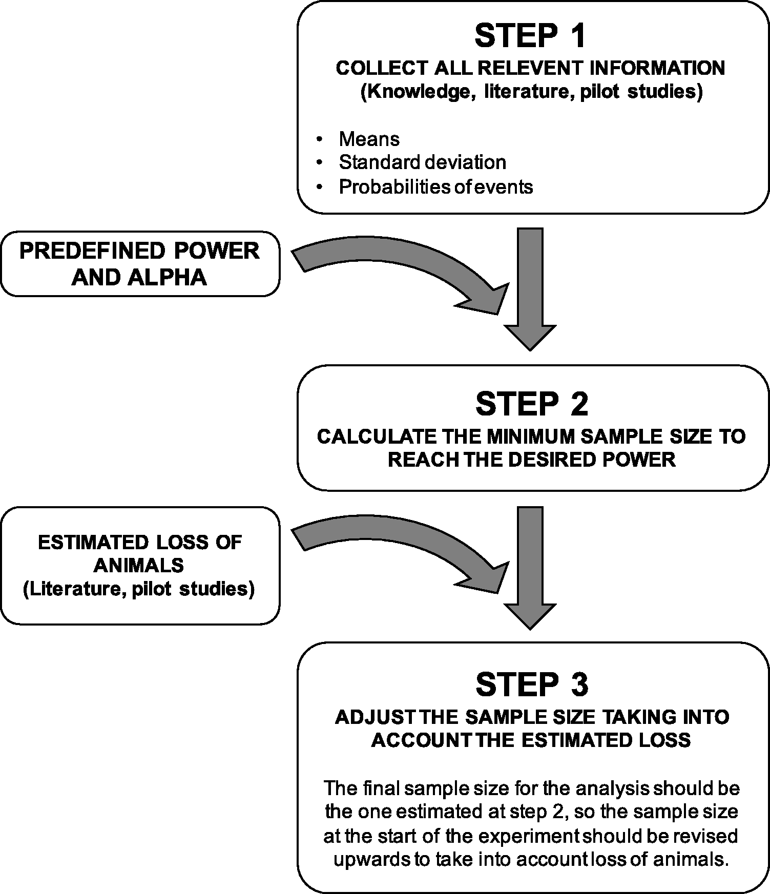

In the second step, the minimum sample size to reach the predefined power (see Recommendation 3) is calculated, usually using a computer assisted tool such as G*Power (www.gpower.hhu.de). This calculation utilises the values of the parameters collected during the previous step in accordance with the planned statistical procedure that will be performed.

The third and last step consists of adjusting the estimated sample size upwards by considering the anticipated severe events. For example, if a sample size calculation indicates 10 animals, and it is anticipated that 10% of animals will die because of treatment and therefore not be statistically exploitable, one extra animal should be added into the experimental design.

Justification of sample size by habits, i.e. the sample size used in the laboratory for years, is not advised; many parameters, such as species, strains, providers, variability, machines, or exact protocols change over time. Similarly, whenever possible, it is recommended to avoid sample sizes based only on the type of experimental technique to be done since central values, SDs and event probabilities are a function of the exact variable of interest in addition to the technique itself. For example, deciding that western-blot analysis will always use extracts from five animals in an entire project that investigates different families of proteins may result in unreliable results due to the inconsistent SD of protein content across protein families. If only one sample size must be chosen in the whole research project, it should be computed using the variability of the most inconstant variable, such as a target protein for example, this can be determined through systematic review of the literature or using a pilot study.

Finally, it is worth mentioning that small samples not only considerably reduce power and are consequently a large source of false negatives, but they also inflate the false discovery rate (FDR), which is the expected proportion of false positives in the declared significant results. ³¹ It is more likely to collect a series of similar and non-representative observations by chance alone in a small sample. Similarly, small sample sizes induce a risk of inflated effect size estimates. ⁴ Therefore, small p-values should always be considered possible false positives if small samples are used, even in the presence of very large effect sizes.

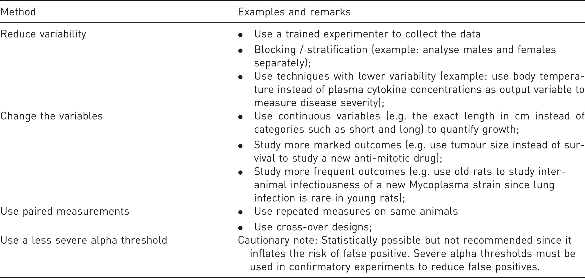
Recommendation 5: Consider options to increase power and precision without increasing sample size

Sample size is positively correlated with power, theoretically prompting for larger samples in animal research. However, the ‘3Rs’ (replace, refine and reduce) provide a framework for reasonable and humane animal research and require (alongside financial and logistic restrictions) that the number of animals included should be reduced to the minimum that allows the experiment to meet the objectives of the research. The final sample size is therefore the result of a tradeoff between the statistical need for high power and the practical constraints of research. Although strongly connected, the notions of power and sample size are not strictly interdependent and can be treated separately. In inferential statistics, additional parameters beyond sample size have an important impact on power. These include: the spread (SD) of the variable of interest when the variable is continuous; the probability of successful events for dichotomous variables; and the desired alpha. In observational studies, in which the objective is often to quantify a variable as precisely as possible, the concept of power is irrelevant and sample size calculation answers the question ‘what is the minimum number of observations needed to have a confidence interval of a certain width’? Similarly, the SD of the variable of interest or probability of events influence the width of confidence intervals. Therefore, an investigator may legitimately attempt to increase the statistical power or precision of a research design without increasing (even while reducing) the sample size (Table 1).

Table 1.

Examples of methods for improving power without increasing sample size.

Method	Examples and remarks
Reduce variability	• Use a trained experimenter to collect the data
	• Blocking / stratification (example: analyse males and females separately);
	• Use techniques with lower variability (example: use body temperature instead of plasma cytokine concentrations as output variable to measure disease severity);
Change the variables	• Use continuous variables (e.g. the exact length in cm instead of categories such as short and long) to quantify growth;
	• Study more marked outcomes (e.g. use tumour size instead of survival to study a new anti-mitotic drug);
	• Study more frequent outcomes (e.g. use old rats to study inter-animal infectiousness of a new Mycoplasma strain since lung infection is rare in young rats);
Use paired measurements	• Use repeated measures on same animals
	• Use cross-over designs;
Use a less severe alpha threshold	Cautionary note: Statistically possible but not recommended since it inflates the risk of false positive. Severe alpha thresholds must be used in confirmatory experiments to reduce false positives.

Recommendation 6: Avoid sequential sampling and optional stopping

An important cautionary note must be issued here regarding the sequential addition of new animals to an apparently underpowered design that seems to give a ‘trend close to significance’. So-called sequential sampling occurs when not all animals are sampled at the same experimental time but are rather added sequentially. This approach may be justified for practical reasons when the full sampling cannot be done on one time point, but it is not recommended to perform the statistical analysis before the predefined sample size is reached. p-Values are variable and will sometimes cross the alpha threshold by chance only. ²⁷ Thus, performing the statistical analysis only when the predefined total number of animals is reached, corresponding to the estimated sample size, ensures the acquisition of the sought power while preventing researchers to stop the sampling process when an ‘expected’ p-value is obtained. Otherwise, sequential sampling results in optional stopping, which is a form of p-hacking, ³² and may result in deeply biased conclusions with inflated chance of false positives (Table 2).

Table 2.

Definition and examples of p-hacking.

p-Hacking: collection or selection of data or statistical analyses until “non-significant” results become “significant”
Examples:
• Stop collecting data once p < α
• Perform many tests but report only those with p < α
• Deciding whether to include or exclude outliers after the analysis to reach p < α
• Transform or rearrange treatment groups after the analysis to reach p < α

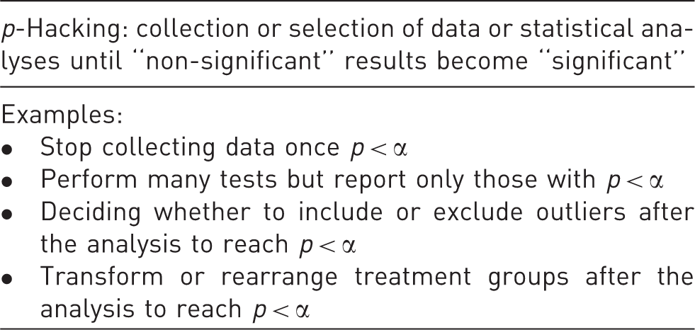
Nevertheless, experimental design may be adaptive in certain situations where the experimenter needs to review and analyse the results before the study reaches the predefined power. This includes the need to monitor remarkable benefits or unacceptable harmful effects, both prompting an early discontinuation of the protocol on ethical grounds. These interim analyses can be implemented, which are methods initially developed for clinical trials. However, it is vital not only that interim analyses are decided during the design phase, including the number of times the investigator will look at the data, but also that a correction is applied to the alpha threshold to prevent the uncontrolled inflation of false positives.^33,34

Statistical analysis

Recommendation 7: Do not use p-values uncritically

In hypothesis testing, statistical analyses almost invariably culminate with p-values, which illustrates the entrenched culture that so-called significant p-values are compulsory and sufficient to reveal a difference or a relationship. The computation of a p-value is often reduced to a binary “yes-or-no” test based on whether p is below an arbitrary alpha limit (usually 0.05). The exact p is not deemed meaningful, as opposed to the statistical significance. However, a “scale of evidence” is paradoxically usually chosen in the form of multiple thresholds, typically at 0.05, 0.01 and 0.001. This paradigm based on a deeply flawed logic disguises the probabilistic substance of statistics that only estimates uncertainty and gives significant p-values a false impression of truth.^5,6

The definition of the p-value is the probability of getting an effect (difference or correlation) of at least the observed magnitude if the null hypothesis H₀ (that posits no difference or correlation) is true. This definition is implicitly and wrongly confused with the probability of H₀, and p-values close to 0 are considered indicator of the improbability of H₀. ⁶ It is very important to keep in mind that the p-value does not indicate the probability of the tested hypothesis. When p = 0.05 the probability of H₀ to be true is often higher than 5%, ³⁵ but the formal demonstration of this is beyond the scope of this article. One way of thinking about this point is to understand that if p-values were a faithful reflection of the truth and of the probability of H₀, repeated samplings of compared populations would give near p-values. However p-values are extremely variable, especially for small samples, because sampling is inconsistent.^27,36 To get a better understanding of this concept, it is possible to imagine the following example. An experimenter makes a mistake after a syringe mislabeling and treats two groups of rats with the exact same treatment, collects the variable of interest (e.g. blood pressure) and decides to compute p-values. The probability of the null hypothesis is p(H₀) = 1 since there is no doubt about the impossibility of an effect. Nevertheless, sampling inconsistency generates samples with slightly divergent statistics even though all rats underwent the same treatment. Consequently, the comparisons will give a wide variety of p-values that will only occasionally approach 1 and will even sometimes be below 0.05 by chance. Therefore, none of the computed p-values will reflect the actual probability of H₀, which is 1.

Another frequent misconception is the belief that the magnitude of the effect is commensurate with the value of p. p-Values provide no information about effect sizes or the magnitude of the effect, but simply give the strength of the evidence against the null hypothesis. For example, increasing the sample size tends to make p-values shrink mathematically although the magnitude of the biological effect is strictly the same.

From the above, the following guidelines are given: 1. use the conditional tense even when in case of small p-values; 2. avoid the word significant alone and prefer the idioms statistically significant, statistically convincing or statistically likely; 3. whenever possible, draw conclusions on effect sizes alongside exact p-values rather than significant thresholds only; 4. if a threshold is used, disclose only one value and avoid the use of a gradual scale of thresholds to indicate apparent increase in statistical significance.

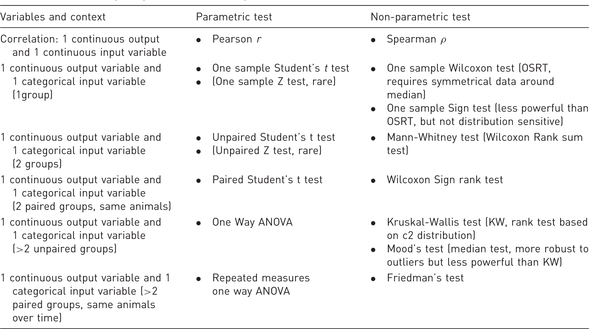
Recommendation 8: Make an informed choice between parametric and non-parametric tests

The arsenal of tests and their variants is vast and one possible decision is the choice between parametric and non-parametric tests, the full descriptions of which are precluded by obvious space limitations in this article. The most frequent tests of both categories are indicated in Table 3 and the decision algorithm to decide whether to select one type or the other is summarised in Figure 4. Briefly, the power of parametric tests is generally higher but several assumptions must be verified otherwise the test readouts may be invalid and a reduction of power may be observed.^37,38 Parametric assumptions are the independence of intragroup observations, homoscedasticity (equality of variances), normality of the sampling distribution of the means and absence of outliers.

Table 3.

The most frequent parametric and non-parametric tests.

Variables and context	Parametric test	Non-parametric test
Correlation: 1 continuous output and 1 continuous input variable	• Pearson r	• Spearman ρ
1 continuous output variable and 1 categorical input variable (1group)	• One sample Student’s t test • (One sample Z test, rare)	• One sample Wilcoxon test (OSRT, requires symmetrical data around median) • One sample Sign test (less powerful than OSRT, but not distribution sensitive)
1 continuous output variable and 1 categorical input variable (2 groups)	• Unpaired Student’s t test • (Unpaired Z test, rare)	• Mann-Whitney test (Wilcoxon Rank sum test)
1 continuous output variable and 1 categorical input variable (2 paired groups, same animals)	• Paired Student’s t test	• Wilcoxon Sign rank test
1 continuous output variable and 1 categorical input variable (>2 unpaired groups)	• One Way ANOVA	• Kruskal-Wallis test (KW, rank test based on c2 distribution) • Mood’s test (median test, more robust to outliers but less powerful than KW)
1 continuous output variable and 1 categorical input variable (>2 paired groups, same animals over time)	• Repeated measures one way ANOVA	• Friedman’s test

Figure 4.

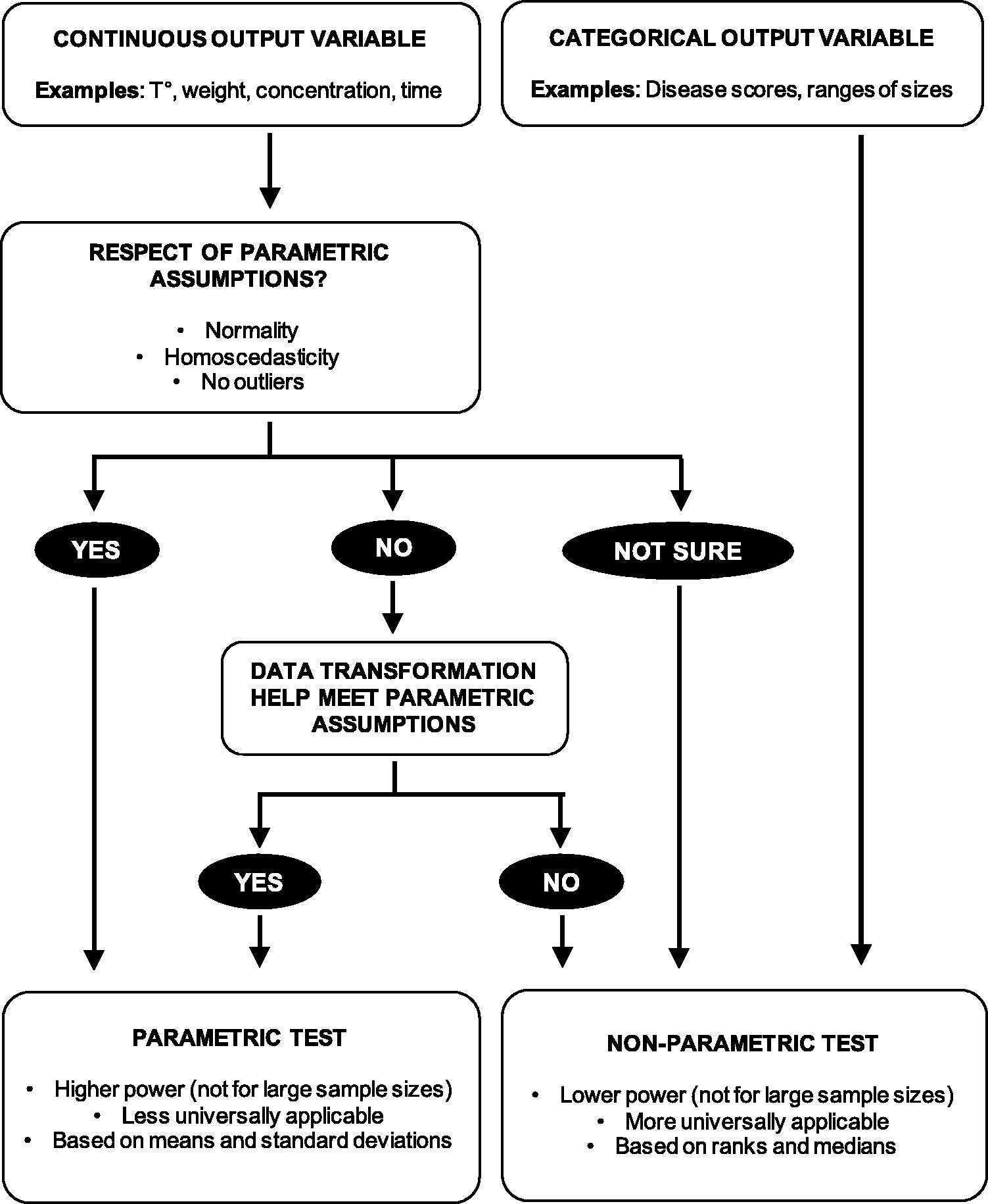
Decision algorithm to help chose between parametric and nonparametric tests.

Homoscedasticity can be verified by several statistical methods such as F-test, Levene’s test or Goldfeld-Quandt test. Similarly, there is a widespread yet questionable culture of testing normality using specific tests such as Kolmogorov-Smirnov or Shapiro-Wilk tests. However, recommendation is given here not to use normality tests due to the usual poor understanding of the implication of their null hypothesis (that the data is compatible with normality). In the common case of low power caused by small samples, no conclusion should be drawn but it is frequent that the resulting high p-values are wrongly interpreted as a testimony of normality. Conversely, in overpowered designs, these tests tend to always give very small p-values, apparently indicating a departure from normality that dismisses parametric tests, simply because many biological measurements are naturally not perfectly normally distributed (e.g. log-normally distributed). It is therefore advisable to avoid normality tests and to utilise other approaches such as Q-Q plots or common knowledge that a known pattern or a natural limit exists, to assess the possible departure from normality. In addition, it is important that the assumption of normality does not apply to the data or the population but rather to the sampling distribution of the mean which is the probability distribution of the means upon multiple samplings. Finally, when outliers are present parametric tests should be avoided due to the influence of extreme values on means, SDs and normality. This is particularly the case when outliers are present in one group or in in one direction of the data only.

In case parametric methods seem inappropriate due to non-normal residuals, the researcher may decide to transform the data to meet the parametric requirements. This might be a valuable alternative in case high power must be retained or if there is no satisfactory non-parametric solution. Common transformations when data are skewed include square root, cube root and log (note that since log is not defined for 0 and negative numbers, a constant must be added to make them all positive before log transformation). Data transformation has been introduced and reviewed by others and we invite the reader to consult the corresponding references.^39–42

If the data does not meet parametric assumptions even after data transformation or if the output variable is not on a continuous scale, non-parametric tests can be used. Non-parametric tests have less assumptions but are not assumption-free. For example, they are similar to parametric tests in their need for independence of intragroup observations. Non-parametric tests are rank tests, which means they proceed by ranking the values in the data and the logic of their null hypothesis is that the observed order of the individual data was obtained by chance only due to random sampling. Therefore, means and SDs are not informative and outliers are not considered nuisance since their rank is not influenced by their distance from the mean. Non parametric tests are thus more universally applicable but the cost for not using the above-mentioned information is threefold: 1. non-parametric tests tend to generally have lower power than their parametric counterparts; 2. p-values are not a function of the exact individual values and very large differences between groups can give similar p-values as small differences, if ranks are the same; and 3) p-values are not on a continuous scale but can only take discrete values since the combinations of ranks is limited in number.

Recommendation 9: Unless you can predict the direction of an effect and are interested in that direction only, use two-tailed tests

Several tests offer a choice between one-tailed or two-tailed options. In summary, one-tailed tests are employed when the possibility of an effect supports the hypothesis in only one direction (e.g. whether treated animals display a convincingly higher value than the control group), whereas two-tailed tests are used when the interest is bidirectional (e.g. whether treated animals display a convincingly different value than the control group, higher or lower). In other words, a researcher can use a one-tailed test if the possible effect is both scientifically interesting in only one direction in the context of the posed biological hypothesis and simultaneously predicted to occur in that direction only. One-tailed tests use the same predefined alpha threshold (usually 5%) but do not split this percentage over the two tails. Instead, they use the 5% area under the curve only in one tail, largely increasing power in that direction. There is a long-standing debate about the use of one-sided tests and contradictory recommendations may be found in the literature.^43–46 One frequent misuse of these tests is the post-hoc decision to (re)analyse the data with a one-tailed test to increase power having observed the direction of the effect and concluding that findings in the other direction do not occur. This approach is a form of p-hacking and is not acceptable. In the Nayman-Pearson approach of NHST, hypotheses must be generated prior to looking at the data, not after. Since my view is that being more conservative is preferable over inflating the risk of false positive results, I recommend to use two-sided tests or to call in a statistician if a one-tailed approach is considered (see Recommendation 1).

Recommendation 10: Correct (correctly) for multiple comparisons

For one comparison (i.e. two groups), the chance of concluding a difference although there is none is the alpha threshold, and is set by the experimenter/statistician (by arbitrary convention usually at 0.05 in life sciences). When more than one statistical test is performed to compare more than two groups, some comparisons may give p-values less than the alpha threshold by chance only, even if there is no actual difference (i.e. all null hypotheses are true). In this case, the chance of observing at least one significant comparison although none exists is not alpha but is called the family-wise error rate (FWER, the family being the total series of comparisons). The FWER is higher than alpha and keeps on inflating rapidly as the number of comparisons increases (Table 4 shows the FWER for alpha = 0.05). The FWER reaches 53.7% when 15 tests are performed (corresponding to 6 groups) and 90.1% for 45 comparisons (corresponding to 10 groups). In other words, if 10 experimental groups are compared pairwise with no correction, the experimenter has 90.1% of chance of finding at least one “significant” result by chance only. Solving this problem becomes vital for such approaches as omics or brain imaging, which make it feasible to perform thousands or millions of statistical tests.

Table 4.

FWER as a function of the number of comparisons (tests) performed.

Number of comparisons	FWER
1	0.050
2	0.098
3	0.143
4	0.185
5	0.226
10	0.401
15	0.537
45	0.901

FWER: Family-wise error rate.

There is no universally applicable approach for dealing with the issue of multiple comparisons since the choice of the method depends on the specificities of the experiment design. However, corrective strategies must be applied to reduce the chances of false positives. Some approaches (e.g. Bonferroni, Sidak corrections) attempt to control the FWER (at 0.05) by making the alpha threshold for each comparison more conservative as the number of tests increases. Other techniques (e.g. Benjamini-Hochberg procedure) perform an adjustment of the p-values aiming at controlling the FDR, which is a proportion of false positives among the significant results. Finally, ANOVA is global (omnibus) test on all the groups of the input variable that determines if among all these groups, at least one may be considered divergent from the others, the exact identification of this latter requires a complementary procedure.

I will not proceed further into the exhaustive listing of methods that aim to correct for multiple comparisons, I invite the reader to consult a statistician if necessary (see Recommendation 1).

Presentation and reporting

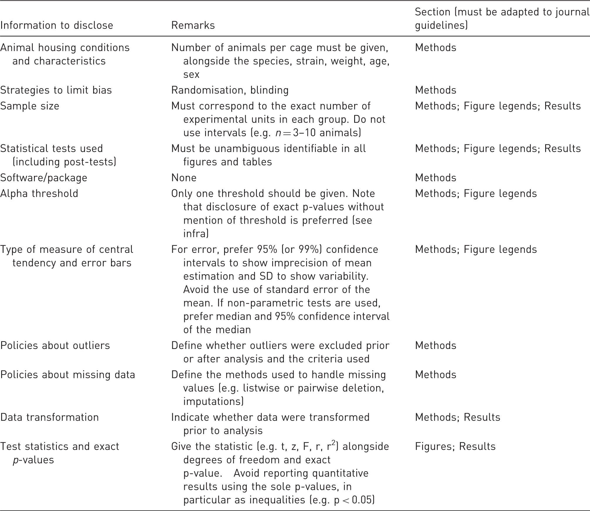
Recommendation 11: Disclose all information needed for the understanding and replication of the study

Scientific reports must enable the reader to critically evaluate and reproduce the study. In animal research, the reference document for reporting is the ARRIVE guidelines, ⁴⁷ whose checklist is available online (https://www.nc3rs.org.uk/arrive-guidelines). All information related to the methods and results must be disclosed. Disclosure about the design includes the sampling methodology, policy with respect to blinding and randomisation as well as the species, strain, number, sex, age and housing conditions of animals (Table 5). The given sample size must refer to the number of independent observations collected (see Recommendation 2), which ultimately are used to compute the variability of the dataset and should not be given as an interval (e.g. n = 3–15 animals) or an inequality (e.g. n > 3). The number of technical replicates must be unambiguously indicated, if applicable. The full statistical procedures must be disclosed including the software used, the statistical tests (including the post-tests used after an omnibus procedure), whether a correction for multiple comparisons has been performed, the alpha threshold and the nature of the error bars. The most practical way to gather all above-listed statistical information is to include a paragraph dedicated to experimental design, biostatistics and data analysis.

Table 5.

Description of statistical information to disclose in publications and related sections.

Information to disclose	Remarks	Section (must be adapted to journal guidelines)
Animal housing conditions and characteristics	Number of animals per cage must be given, alongside the species, strain, weight, age, sex	Methods
Strategies to limit bias	Randomisation, blinding	Methods
Sample size	Must correspond to the exact number of experimental units in each group. Do not use intervals (e.g. n = 3–10 animals)	Methods; Figure legends; Results
Statistical tests used (including post-tests)	Must be unambiguous identifiable in all figures and tables	Methods; Figure legends; Results
Software/package	None	Methods
Alpha threshold	Only one threshold should be given. Note that disclosure of exact p-values without mention of threshold is preferred (see infra)	Methods; Figure legends
Type of measure of central tendency and error bars	For error, prefer 95% (or 99%) confidence intervals to show imprecision of mean estimation and SD to show variability. Avoid the use of standard error of the mean. If non-parametric tests are used, prefer median and 95% confidence interval of the median	Methods; Figure legends
Policies about outliers	Define whether outliers were excluded prior or after analysis and the criteria used	Methods
Policies about missing data	Define the methods used to handle missing values (e.g. listwise or pairwise deletion, imputations)	Methods
Data transformation	Indicate whether data were transformed prior to analysis	Methods; Results
Test statistics and exact p-values	Give the statistic (e.g. t, z, F, r, r2) alongside degrees of freedom and exact p-value. Avoid reporting quantitative results using the sole p-values, in particular as inequalities (e.g. p < 0.05)	Figures; Results

Recommendation 12: Chose correct graphical display for your quantitative results

The choice of a graphical representation must be made judiciously, with the aim of giving the most information that informs about patterns (numerical data can be given using tables). Whenever possible, bar graphs should be avoided since they convey very little information about actual data distributions. Instead, scatter plots showing all individual values should be used for small samples and more refined representations should be preferred such as box/whisker plots or violin plots for larger samples. SEMs should not be used as indicators of error since they are misleading representations and should be replaced by 95% confidence interval of the mean or median to show the interval in which the mean or median will be located in 95% of future samplings, or the SD should be used to show variability.

Conclusion

The present series of recommendations exposes simple and inexpensive measures aiming to improve the quality of biostatistics in animal research. This review focuses exclusively on biostatistics and therefore extends the existing guidelines about experimental design and reporting in animal research. ⁴⁷ It is important to realise that the use of proper statistics is not only a matter of data analysis, but ranges from experimental design to data presentation and should therefore be carefully addressed throughout the research project. Furthermore, it is worth mentioning that many aspects of scientific research may contribute to the lack of reproducibility, with flawed biostatistics being only one of them. The author therefore encourages researchers to use additional means that contribute to better reproducibility, including improved reporting of conflict of interest as well as open-access and preprint policies. The scientific community should adopt better practices that reward good experimental design and stop creating strong incentives to publish only “statistically significant” results. The author therefore encourages journals to be at the forefront of this action and to support statistically-relevant initiatives such as confirmatory studies or alternatives to the overconfidence about p-values and NHST.