Sage Journals: Discover world-class research

Abstract

German

Spanish

French

Underpowered experiments have three problems: true effects are harder to detect, the true effects that are detected tend to have inflated effect sizes and as power decreases so does the probability that a statistically significant result represents a true effect. Many biology experiments are underpowered and recent calls to change the traditional 0.05 significance threshold to a more stringent value of 0.005 will further reduce the power of the average experiment. Increasing power by increasing the sample size is often the only option considered, but more samples increases costs, makes the experiment harder to conduct and is contrary to the 3Rs principles for animal research. We show how the design of an experiment and some analytical decisions can have a surprisingly large effect on power.

Keywords

experimental design power reproducibility sample size statistics

Introduction

Statistical power is the probability of detecting a true effect, and therefore when experiments have low power, a true effect or association is hard to find.^1,2 In addition, with low power, small effects will only be statistically significant when the effect size is overestimated (or if the within-group SD is underestimated).^3–5 In other words, the correct qualitative conclusion might be reached (there is an effect) but the magnitude or strength of the effect is overestimated.⁴ A final and less appreciated consequence of lower power is that as power decreases, so does the probability that a statistically significant result represents a true effect.^2,6–8 The probability that a significant result is a true effect is often called the positive predictive value and is calculated as the number of true positive results divided by the total number of positive results (the sum of true positive and false positive results). Since true positives are harder to detect as power decreases, the probability that p < 0.05 represents a true positive also decreases (see Wacholder et al. and Ioannidis for further details).^6,7 Thus, lower power has a triple-negative effect on statistical inference.

Statisticians and scientists have recently been arguing for a more stringent significance threshold of 0.005 because the traditional 0.05 threshold provides little evidence against the null hypothesis.^9–13 If journals start requiring a lower threshold for significance, the power of all experiments will be further reduced, exacerbating the above problems. By way of example, suppose we are conducting a two-group experiment with independent samples in each group and want 80% power to detect a difference of 1.25 (arbitrary) units. Assume the within-group SD is 1 and the significance threshold is 0.05. We require 11 samples per group, or 22 in total. If the significance threshold is reduced to 0.005, 38 total samples are required: a 71% increase in sample size. If only 22 samples are used with the more stringent 0.005 significance threshold, the power of the experiment is only 44%.

To increase power, many researchers only consider increasing the sample size (N). Indeed, standard power and sample size calculations in textbooks and review articles suggest that the only option to increase power is to increase the number of samples. The structure of the design of the experiment is taken as given, the probability of a Type I error (false positive) is set to $α = 0.05$ , and the power is usually fixed to 80% or 90%. The effect size is the smallest effect that is biologically or clinically meaningful and that the researcher would like to detect, and the within-group SD is derived from pilot studies, published results or an educated guess (in practice, and not recommended, the effect size and SD are often adjusted to give the sample size that investigators were planning to use all along).^14,15 This only leaves N to be adjusted to meet the desired power. We assume, as is standard for most traditional frequentist analyses, that the sample size is determined before the experiment is conducted and cannot be changed during the experiment. This inflexible approach is inefficient because experiments cannot be stopped early if a definitive conclusion is reached based on a predefined criterion. Although methods have been developed for the analysis of such ‘adaptive’ designs, they are not considered here.^16–18

Increasing the sample size makes the experiment more expensive, harder to conduct, and has ethical implications for animal experiments. Also, it is often difficult to hold everything else constant while increasing N. A small experiment could be run all at once, but a larger experiment may need to be run in smaller batches: perhaps on two separate days, or by two researchers. ‘Day’ and ‘researcher’ are technical factors that could influence the outcome and may need to be included as variables in the analysis. If so, the design of the experiment now differs from the design used for the power calculation. Similarly, data from a small experiment may be collected over a short period of time (e.g. 1 or 2 hours), making circadian effects negligible. A larger experiment may need to collect data over a longer period, and now circadian effects may become more pronounced. The design of the experiment now needs to change to accommodate the circadian effects; for example, by using time as a covariate or blocking factor.¹⁹ This is again a different experiment to the one used for the power calculation.

Simple options are available to increase power – often dramatically – while keeping the sample size fixed. Or coming from the other direction, certain design and analytical options should be avoided to prevent loss of power. Four options are described below that apply to many biological experiments and other options for increasing power are described in Lazic;¹⁹ for example, ensuring that predictor variables are uncorrelated, optimising the spatial and temporal spacing of observations, and using blocking and covariates to reduce noise. The R code for the examples shown in this paper is provided as supplementary material.

Trade-offs are inevitably required when planning an experiment, and defining a key question or hypothesis enables the experiment to be designed to maximise the chance of success, but at the cost of being unable to address other questions. Hence, the first step is to clearly define the key question that the experiment will answer. This may sound trite, but consider an experiment testing a new compound in an animal model of a disease. The key questions could be:

Is the compound active (does it work at all)?

Is the compound active at a specific dose?

What is the minimum effective dose?

What dose gives half of the maximum response (the Effective Dose 50% or ED50)?

What is the relationship between dose and response?

Is one dose better than another?

No design is optimal for answering all of these questions; some designs are better for some questions and other designs are better for other questions. Once the question or hypothesis is defined, the four points below can be used to plan the experiment.

Use fewer factor levels for continuous predictors

In experiments with continuous predictors such as dose, concentration, time, pH, temperature, pressure, illumination level and so on, how do we decide on the minimum and maximum levels, the number of points in between, and the specific levels where observations will be made or samples allocated? Some choices are easy, for example, when a minimum value of zero serves as a control condition. The maximum value is also often easy to choose as it is the upper limit that we are interested in testing or learning about. But what about the points between the minimum and maximum? The places where observations are made (minimum and maximum plus intermediate points) are called the design points.²⁰

To illustrate how the number of design points affects the power, we compare four designs with 2–5 equally spaced design points (experimental groups) and a fixed total sample size of 20. Assume that the dose of a compound is the factor of interest, which ranges from minimum = 0 to maximum = 100. 10,000 data sets were simulated from the true model (Figure 1(a)), which has a maximum response of 40 at dose = 0, and a minimum response of 27 at dose = 100. The variability of the data is shown by the scatter of points around the dose-response line (SD = 9). Data were simulated under each design and analysed with a one-way analysis of variance (ANOVA), testing the first question above: ‘is the compound active at all’? Continuous predictor variables such as dose are often better analysed with linear or nonlinear regression methods,²¹ especially when the form of the relationship is known from theory or background knowledge. A one-way ANOVA is used instead because it is the most common approach in many fields and because it can be used for all designs, including those not considered here.

Figure 1.

Effect of increasing the number of groups. A fictitious example of the relationship between an outcome and the dose of a compound (a). Four designs with the same sample size but with observations taken at different doses are indicated with black circles. For example, design 1 has 10 samples at doses 0 and 100. Increasing the number of groups from 2 to 5 decreases the power for the overall analysis of variance (ANOVA) from 84 to 40% (b). Testing a more specific hypothesis for a trend has improved power compared with an ANOVA analysis, but still loses power with more groups.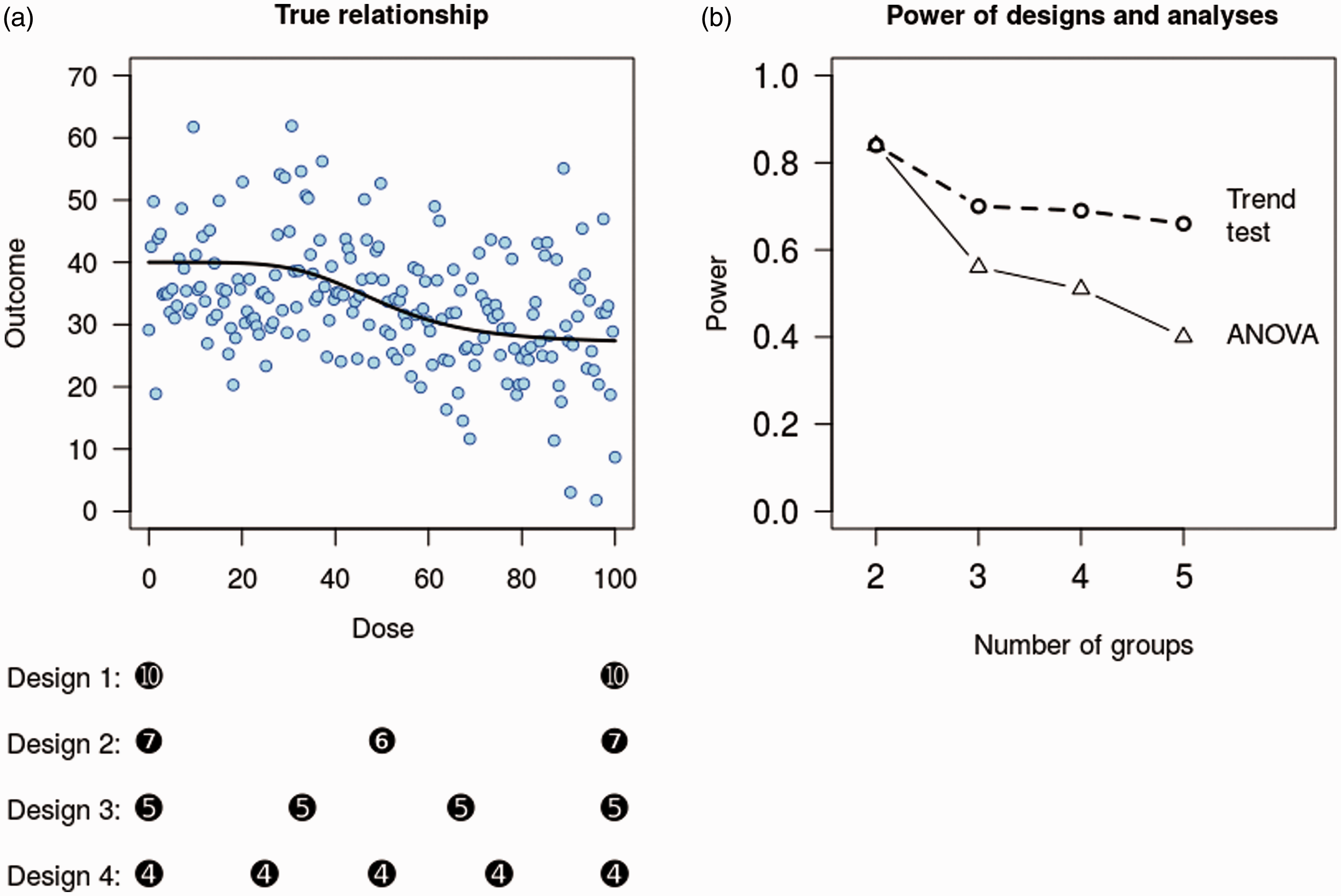

The power for each design is calculated as the proportion of significant results from the ANOVA F-test. Despite the same sample size, the power of these experiments differs greatly (Figure 1(b), ‘ANOVA line’). The power of design 1 with two groups is 84% and steadily decreases to 40% with design 4.

It is clear that using two groups maximises power. But what if the true relationship is not sigmoidal but a ‘U’, inverted-‘U’ or some other complex shape? A design with two groups would be unable to detect such relationships, but if a linear or monotonic relationship is expected, then one additional design point can allow departures from the assumed relationship to be detected (e.g. design 2 in Figure 1).²⁰ Trade-offs are always necessary when designing experiments; while an additional group allows a more complex relationship to be detected, it lowers the probability of detecting a linear relationship if that is indeed the correct one.

If the aim of the study is to answer the second question (‘is the compound active at a specific dose?’), then only the doses in question and the control group are required. Given this research question, a small increase in power can be achieved by shifting a few samples from the treated groups to the control group, compared with an equal number of samples in each group (see Bate and Karp²²). Questions 3–5 are better addressed with a linear or nonlinear regression model as the minimum effective dose or the ED50 are unlikely to be at one of the doses used in the experiment. As nonlinear models interpolate between the observed design points, they can provide an estimated value anywhere in the design space. Nonlinear models can benefit from having more than the five design points used here and are often in the 8–10 range.^23,24 Addressing question 6 (‘is one dose better than another?’) does not even require the control group, although controls inform us about the state of the experimental system and should be retained.²⁵ Nevertheless, the control group could have fewer samples, which are then transferred to the treated groups to increase the power of the comparisons between the treated groups. This decreases the power of treated versus control group comparisons, illustrating again how the aim of the experiment or the question asked influences the design. Berger and Wong discuss a wider range of designs and how they affect power for different types of relationships.²⁰

ANOVA analyses are often followed by post hoc tests comparing group means. Power also decreases for post hoc comparisons as the number of groups increases. For example, the power for the 0 versus highest dose group comparison in design 5 is only 45%, and this does not adjust for multiple comparisons, which would reduce power further. The power for the 0 versus highest dose group in design 1 is 85%, the same as the overall ANOVA, because there are only two groups and so a post hoc test is unnecessary.

A final point to maximise power is ensure that the predictor variable covers a wide enough range; for example, the compound would appear to have no effect if the maximum dose tested in the experiment was 30.

Use a focused hypothesis test

A second way to increase power is to test a specific hypothesis instead of a general ‘are there any differences?’ hypothesis. For the simulated example above, the ANOVA analysis can detect any pattern of differences between groups, but the trade-off is that it has less power to detect any specific pattern. If we expect the outcome to either steadily increase or decrease as the dose increases, then a focused test of this pattern is more powerful (Figure 1(b), ‘trend test’ line).

With two groups, the power of the trend test is identical to the ANOVA analysis (both are equivalent to a t-test), but with five groups (design 4) the power of the trend test is 66%, compared with 40% for the ANOVA analysis. Trend tests are available in most statistical packages (even if they are not labelled as such) and usually require that the predictor variable – dose in this case – is treated as an ordered categorical factor. The output from such an analysis should include the test for a linear trend, often called the ‘linear contrast’ or similar. Alternatively, treating dose as a continuous variable and analysing the data with a regression analysis instead of an ANOVA is another option that has high power as well as other advantages.²¹

Don’t dichotomise or bin continuous variables

Dichotomising or binning refers to taking a continuous variable – either an outcome or predictor variable – and reducing it to a categorical variable based on a threshold such as the median (e.g. low/high or low/medium/high). This practice is common, despite the many papers warning against it. Dichotomising variables reduces power, can bias estimates and can increase false positives.^21,26–39

This recommendation does not contradict the first point about using fewer factor levels for continuous variables because, when designing an experiment, we can only take observations at discrete points within the design space, and so there will be some discretising. But a continuous variable that we record – either an outcome or a predictor – can take any value. The argument here is that if you have the continuous values, the costs outweigh the benefits of converting it into a categorical variable.

To illustrate this point, Figure 2 shows data for 50 samples that have a correlation of 0.4. These are naturally analysed with a Pearson correlation or linear regression (solid line), both of which give p = 0.002 for the association. If the variables are dichotomised at their median (dashed lines), the number of data points falling in each quadrant can be counted (numbers in grey boxes), forming a 2 × 2 table. This doubled-dichotomised data is commonly analysed with a $χ^{2}$ test or Fisher’s exact test, and the $χ^{2}$ test gives p = 0.024, almost 10 times larger than the regression analysis. To estimate the reduction power when using the $χ^{2}$ test, 10,000 data sets like the one in Figure 2 were simulated with N = 50 and a correlation of 0.4. Analysing the continuous values with a regression analysis had 84% power, while binning and using the $χ^{2}$ test reduced power to 34%.

Figure 2.

Analysis of continuous and binned data. A regression analysis (black line) gives p = 0.002. Binning the data with a bivariate median split (dashed lines) and analysing the number of samples in each quadrant (grey boxes) with a 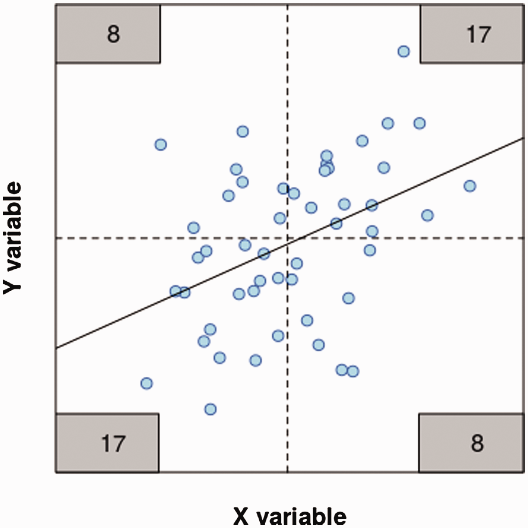$χ^{2}$ test gives p = 0.024. The power of the $χ^{2}$ test is only 34%, compared with 84% for the regression analysis.

Data are sometimes binned because the relationship between the predictor and the outcome variable is nonlinear and a simple regression or correlation analysis would be unsuitable. Binning the data is still a poor option and frequently a simple alternative is available. For example, Spearman’s rank correlation tests for a monotonic relationship between two variables, and there is no requirement for a linear relationship or assumptions about the distribution of the variables. Alternatively, a ‘U’, inverted-‘U’ relationship between the variables might be modelled with a quadratic term in a regression model, which is available in all statistical software. The take home message of this section is that it is almost always preferable to analyse a continuous variable directly instead of reducing it to a categorical variable.

Cross your factors, don’t nest them

The levels of an experimental factor are either (a) set by the researcher, (b) a property of the samples or (c) a technical aspect of how the experiment is conducted. For example, the dose of a drug that an animal receives is controlled by the researcher, while the sex of the animal is a property of the animal. If the experiment is conducted over multiple days or by multiple researchers, then day and researcher are technical factors. Factor arrangement refers to how multiple factors relate to each other within the experimental design, and there are three possibilities.

When two factors are completely confounded, levels of one factor always co-occur with the same levels of the other factor; for example, if all the control animals are run on the first day and all the treated animals are run on the second day. Confounding a treatment effect that we are interested in testing with an uninteresting technical effect is never a good idea because it is impossible to attribute any differences between treatment groups to the effect of the treatment; differences may have arisen from the day-to-day variation. To conclude anything about a treatment effect we would have to assume that the effect of day is zero, and therefore this arrangement should be avoided.

The second possibility is a crossed or factorial arrangement, which occurs when all levels of one factor co-occur with all levels of another factor and is the most common arrangement in experimental biology. The final possibility is a nested arrangement, where levels of one factor are grouped or nested under the levels of another factor. Figure 3 shows the difference between crossed and nested arrangements. Suppose that we have 16 mice (assume all male for simplicity) from four litters (A–D) and we want to test the effect of a compound at a single dose. Assume that each mouse can be randomly and individually assigned to one of the two treatment groups. Although this is a simple two-group design, we might expect differences between litters and want to take this into account in the design.

Figure 3.

Crossed versus nested designs. An experiment with 16 mice from four litters (A–D) can be randomised to treatment groups either by litter, leading to a nested design (left), or within litter, leading to a crossed design (right).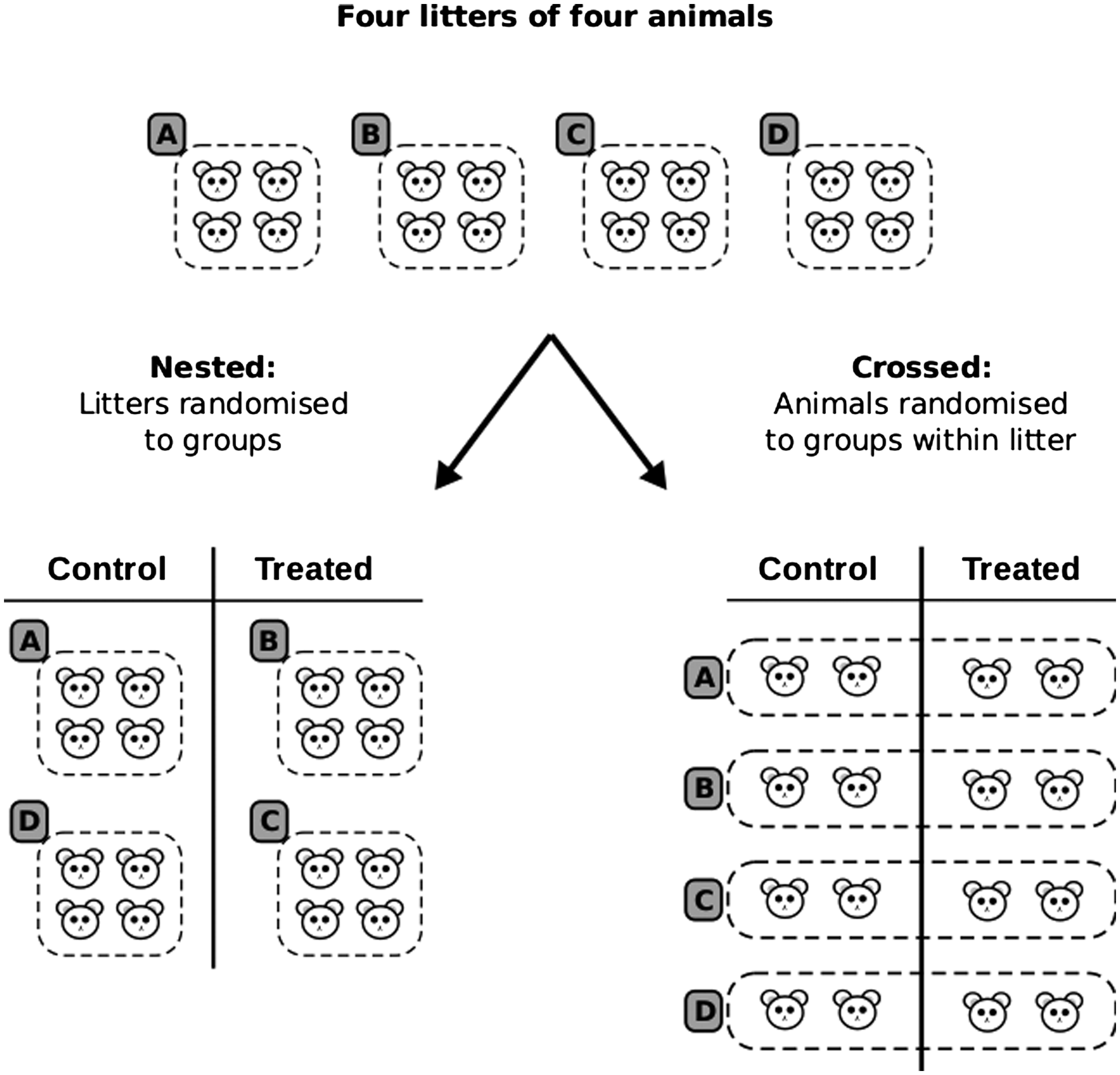

When all animals from a litter are in the same condition, the factor litter is said to be nested under the factor treatment (Figure 3, left). When animals from a litter are spread across both treatment groups, the treatment and litter factors are crossed (Figure 3, right).

The main point here is that the nested arrangement is much less powerful than the crossed one. Figure 4 illustrates the difference in power between the two designs. The litter means are drawn from a normal distribution with an SD of 3, and the values for the individual animals are drawn from a normal distribution with an SD of 0.5. Thus, the litter-to-litter variation is large relative to the variation between animals within a litter. Figure 4(a) shows the data before the application of a treatment, and an immediate danger can be seen with a nested design: if litters A and B end up in one group and C and D in the other, large differences between groups exist at baseline. Hence, nested designs can also potentially lead to more false positive findings.^40,41

Figure 4.

Simulated data for a nested and crossed design. Natural variation between and within litters (a). The nested design compares the effect of the treatment against the high variation between litters, leading to a large p-value (0.14 or 0.57, depending on the analysis) (b). The crossed design compares the treatment effect to the smaller within-litter variation, leading to a much smaller p-value of 0.0007 (c).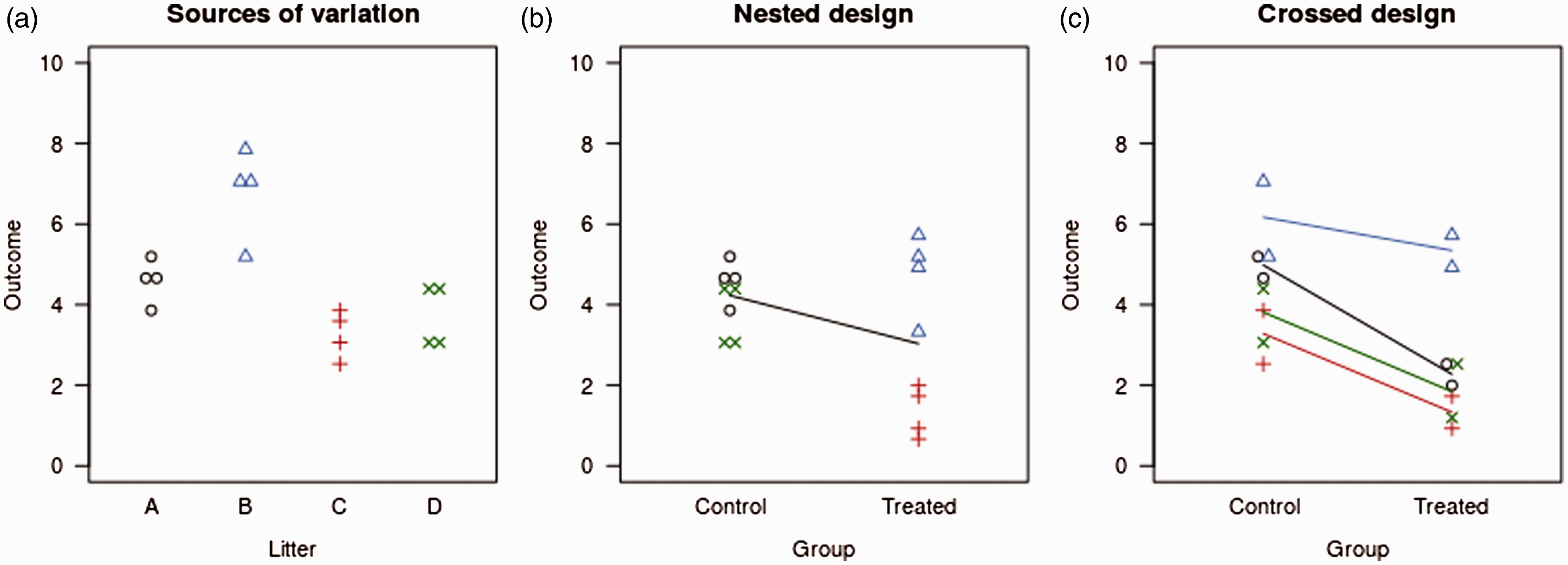

Figure 4(b) shows one possible randomisation of a nested design, where litters A and D end up in the control group and B and C in the treated group. The effect of the treatment in this example is to decrease the outcome by 2 units (note how the control group values of black O’s and green ×’s are identical in Figure 4(a) and (b)). Analysing the data with a t-test gives a p-value of 0.14. However, since the litters were randomised to the treatment conditions and not the individual animals, the litter is a more appropriate experimental unit, that is, the sample size is four litters, not 16 animals.^19,42 One way to conduct this analysis is to calculate the litter average and use these values for a standard statistical test, which gives p = 0.57. Figure 4(c) shows one possible randomisation of the crossed design, with the same effect size of −2 units. Analysis of this design, which includes litter as a variable in the model, gives p = 0.0007 for the effect of the treatment.

To calculate the power of the two designs and both analyses of the nested design, 10,000 data sets were generated with the above characteristics. The nested design that treats animals as the experimental unit has 55% power, and treating the litter as the experimental unit (the more appropriate analysis) has only 7% power. The power of the crossed design is over 99%. These large differences in power exist because the nested design compares the effect size of −2 units against the high litter-to-litter variation (SD = 3), whereas the crossed design compares the effect size against the much smaller variation of animals within a litter (SD = 0.5). With the crossed design, the test for a treatment effect is performed within the litters and hence large differences between litters are irrelevant for testing treatment effects. Litter is used here as a ‘blocking variable’ to remove the unwanted litter-to-litter variation.^40,43

The difference in power between nested and crossed designs become less pronounced as litter effects get smaller, animal variation within a litter gets larger or both. The nested design should be avoided because of low power, more false positives and ambiguity in defining the sample size¹⁹. Unfortunately, nested designs are common because they are often easier to conduct and manage; for example, it’s easier to randomise litters to treatment groups as littermates can be housed together in the same cage.

Other technical variables or properties of subjects such as batches, microtitre plates, cages or other housing structure, body weight, day and experimenter can also be nested or crossed with the treatment effects of interest. These factors need to be carefully arranged to ensure high power and no confounding. The points discussed above can combine to reduce power even further; for example, using a nested design, dichotomising a variable and testing a general hypothesis will have a dramatic loss of power compared with a crossed design, without dichotomisation and testing a focused hypothesis.

Conclusion

Low power continues to undermine many biology experiments, but a few simple alterations to a design or analysis can dramatically increase the information obtained without increasing the sample size. In the interest of minimising animal usage and reducing waste in biomedical research,^44,45 researchers should aim to maximise power by designing confirmatory experiments around key questions, use focused hypothesis tests, and avoid dichotomising and nesting, which ultimately reduce power and provide no other benefits.

Footnotes

Acknowledgements

I would like to thank Deborah Mayo, Frank Harrell and other readers who commented on the pre-print version of this article on bioRxiv or social media.

Declaration of Conflicting Interests

The author(s) declared no potential conflicts of interest with respect to the research, authorship and/or publication of this article.

Funding

The author(s) received no financial support for the research, authorship and/or publication of this article.

References

Maxwell

. The persistence of underpowered studies in psychological research: Causes, consequences, and remedies. Psychol Methods 2004; 9: 147–163.

Button

Ioannidis

Mokrysz

et al.

Power failure: Why small sample size undermines the reliability of neuroscience. Nat Rev Neurosci 2013; 14: 365–376.

Ioannidis

JPA

. Why most discovered true associations are inflated. Epidemiology 2008; 19: 640–648.

Gelman

Carlin

. Beyond power calculations: Assessing type S (Sign) and type M (Magnitude) errors. Perspect Psychol Sci 2014; 9: 641–651.

McShane

Bockenholt

. You cannot step into the same river twice: When power analyses are optimistic. Perspect Psychol Sci 2014; 9: 612–625.

Wacholder

Chanock

Garcia-Closas

et al.

Assessing the probability that a positive report is false: An approach for molecular epidemiology studies. J Natl Cancer Inst 2004; 96: 434–442.

Ioannidis

JPA

. Why most published research findings are false. PLoS Med 2005; 2: e124–e124.

Nuzzo

. Scientific method: Statistical errors. Nature 2014; 506: 150–152.

Berger

Sellke

. Testing a point null hypothesis: The irreconcilability of p values and evidence. J Am Stat Assoc 1987; 82: 112–122.

10.

Sellke

Bayarri

Berger

. Calibration of p values for testing precise null hypotheses. Am Stat 2001; 55: 62–71.

11.

Johnson

. Revised standards for statistical evidence. Proc Natl Acad Sci USA 2013; 110: 19313–19317.

12.

Singh Chawla

. Big names in statistics want to shake up much-maligned P value. Nature 2017; 548: 16–17.

13.

Benjamin

Berger

Johannesson

et al.

Redefine statistical significance. Nat Hum Behav 2018; 2: 6–10.

14.

Schulz

Grimes

. Sample size calculations in randomised trials: Mandatory and mystical. Lancet 2005; 365: 1348–1353.

15.

Bacchetti

. Current sample size conventions: Flaws, harms, and alternatives. BMC Med 2010; 8: 17–17.

16.

Berry

Carlin

Lee

et al.

Bayesian adaptive methods for clinical trials, Boca Raton: CRC Press, 2010.

17.

Schonbrodt

Wagenmakers

Zehetleitner

et al.

Sequential hypothesis testing with Bayes factors: Efficiently testing mean differences. Psychol Methods 2017; 22: 322–339.

18.

Schonbrodt

Wagenmakers

. Bayes factor design analysis: Planning for compelling evidence. Psychon Bull Rev. Epub ahead of print 1 March 2017. DOI: 10.3758/s13423-017-1230-y.

19.

Lazic

. Experimental design for laboratory biologists: Maximising information and improving reproducibility, Cambridge: Cambridge University Press, 2016.

20.

Berger

MPF

Wong

. An introduction to optimal designs for social and biomedical research, Chichester: John Wiley & Sons, 2009.

21.

Lazic

. Why we should use simpler models if the data allow this: Relevance for ANOVA designs in experimental biology. BMC Physiol 2008; 8: 16–16.

22.

Bate

Karp

. A common control group - optimising the experiment design to maximise sensitivity. PLoS One 2014; 9: e114872–e114872.

23.

Motulsky

Christopoulos

. Fitting models to biological data using linear and nonlinear regression: A practical guide to curve fitting, Oxford: Oxford University Press, 2004.

24.

Ritz

Streibig

. Nonlinear regression with R, New York: Springer-Verlag, 2008.

25.

Glass

. Experimental design for biologists, Cold Spring Harbor: Cold Spring Harbor Laboratory Press, 2007.

26.

Barnwell-Menard

J-L

Cohen

. Effects of categorization method, regression type, and variable distribution on the inflation of type-I error rate when categorizing a confounding variable. Stat Med 2015; 34: 936–949.

27.

Bennette

Vickers

. Against quantiles: Categorization of continuous variables in epidemiologic research, and its discontents. BMC Med Res Methodol 2012; 12: 21–21.

28.

Chen

Cohen

Chen

. Biased odds ratios from dichotomization of age. Stat Med 2007; 26: 3487–3497.

29.

Cohen

. The cost of dichotomization. Appl Psychol Meas 1983; 7: 249–253.

30.

Fedorov

Mannino

Zhang

. Consequences of dichotomization. Pharm Stat 2009; 8: 50–61.

31.

Irwin

McClelland

. Negative consequences of dichotomizing continuous predictor variables. J Mark Res 2003; 40: 366–371.

32.

Kenny

Montanari

. Inflation of correlation in the pursuit of drug-likeness. J Comput Aided Mol Des 2013; 27: 1–13.

33.

Maxwell

Delaney

. Bivariate median splits and spurious statistical significance. Quant Methods Psychol 1993; 113: 181–190.

34.

Owen

Froman

. Why carve up your continuous data? Res Nurs Health 2005; 28: 496–503.

35.

Royston

Altman

Sauerbrei

. Dichotomizing continuous predictors in multiple regression: A bad idea. Stat Med 2006; 25: 127–141.

36.

Taylor

. Bias and efficiency loss due to categorizing an explanatory variable. J Multivar Anal 2002; 83: 248–263.

37.

van Walraven

Hart

. Leave ’em alone - why continuous variables should be analyzed as such. Neuroepidemiology 2008; 30: 138–139.

38.

Wainer

Gessaroli

Verdi

. Finding what is not there through the unfortunate binning of results: The Mendel effect. Chance 2006; 19: 49–52.

39.

Kuss

. The danger of dichotomizing continuous variables: A visualization. Teach Stat 2013; 35: 78–79.

40.

Lazic

Essioux

. Improving basic and translational science by accounting for litter-to-litter variation in animal models. BMC Neurosci 2013; 14: 37–37.

41.

Lazic

. Comment on “stress in puberty unmasks latent neuropathological consequences of prenatal immune activation in mice”. Science 2013; 340: 811–811.

42.

Lazic

Clarke-Williams

Munafo

. What exactly is ‘N’ in cell culture and animal experiments? bioRxiv 2018. (in press). DOI: 10.1101/183962.

43.

Festing

MFW

. Randomized block experimental designs can increase the power and reproducibility of laboratory animal experiments. ILAR J 2014; 55: 472–476.

44.

Macleod

Michie

Roberts

et al.

Biomedical research: Increasing value, reducing waste. Lancet 2014; 383: 101–104.

45.

Ioannidis

JPA

Greenland

Hlatky

et al.

Increasing value and reducing waste in research design, conduct, and analysis. Lancet 2014; 383: 166–175.

Four simple ways to increase power without increasing the sample size

Abstract

Keywords

Introduction

Use fewer factor levels for continuous predictors

Use a focused hypothesis test

Don’t dichotomise or bin continuous variables

Cross your factors, don’t nest them

Conclusion

Footnotes

Acknowledgements

Declaration of Conflicting Interests

Funding

References