
Abstract
Objectives:
This article examines the hypothesis that in street robbery location choices, the importance of location attributes is conditional on the time of day and on the day of the week.
Method:
The hypothesis is assessed by estimating and comparing separate discrete location choice models for each two-hour time block of the day and for each day of the week. The spatial units of analysis are census blocks. Their relevant attributes include presence of various legal and illegal cash economies, presence of high schools, measures of accessibility, and distance from the offender’s home.
Results:
The hypothesis is strongly rejected because for almost all census block attributes, their importance hardly depends on time of day or day of week. Only the effect of high schools in census blocks follows expectations, as its effect is only demonstrated at the times and on the days that schools are open.
Conclusions:
The results suggest that street robbers’ location choices are not as strongly driven by spatial variations in immediate opportunities as has been suggested in previous studies. Rather, street robbers seem to perpetrate in the environs of cash economies and transit hubs most of the time irrespective of how many potential victims are around.
Introduction
To be successful, street robbers must attack at the right time at the right place. A place may be good for late-night robbery because there is an abundance of intoxicated persons who are easy targets. But the same place might be a very unattractive target area in the early morning light when people are rushing to their workplaces. A place that is bare on weekends might be full of suitable targets during the rest of the week. The attributes that make places attractive spots for street robbery are not stable but change over daily and weekly cycles. They depend on the daily whereabouts and activities of potential victims and law enforcement. In other words, time of day and day of week set conditions for selecting attractive targets and for avoiding arrest.
Making these claims may seem like pushing at an open door, but the truth is that they are not facts at all. They are hypotheses that have not been as extensively tested as one might expect and where they have been tested they have not consistently been confirmed.
Most research on spatial variation in crime has overlooked the temporal dimension. It explores where crime takes place but ignores when it does. Most research on temporal variation in crime has overlooked the spatial dimension, as it explores when crime takes place but ignores where it does. Notable exceptions that simultaneously address spatial and temporal variation include Ratcliffe (2002), Coupe and Blake (2006), Ceccato and Uittenbogaard (2014), Irvin-Erickson and La Vigne (2015), and Haberman and Ratcliffe (2015). Limitations in data availability are unlikely to be the reason for ignoring either time or place, as both time and place are two widely recorded attributes of crime. Even if the exact timing is not known, it is usually recorded as a time window between starting time and ending time (Ratcliffe 2002).
The hypothesis suggested in the first paragraph is that for street robbers, the importance of a target area attribute is conditional on the time of day and on the day of the week, not because the robber changes his or her preferences but because the target area attributes depend on time of day and day of week, and are outside the robber’s control. This hypothesis is inspired by a rational choice perspective on crime. Rational choice theory, however, is not the only theory predicting temporal variability in where crime takes place. Routine activity theory (Cohen and Felson 1979) emphasizes that the convergence of offenders and targets in both space and time is a necessary requirement for predatory crime. Other theoretical perspectives, including crime pattern theory (Brantingham and Brantingham 1993) and space-time geography (Miller 2005), offer supporting arguments that help us understand why the locations of criminal opportunity vary with daily and weekly tides in human activity.
The present article seeks to contribute to the knowledge about how spatial crime patterns depend on the time of the day and the day of the week. Using data on the city of Chicago, we answer the question whether street robbers’ crime location preferences vary across the hours of the day and across the days of the week. Thereby, we replicate and extend a recent study on street robberies in the city of Philadelphia that addressed a similar question (Haberman and Ratcliffe 2015). The authors investigated whether street robbers’ crime location preferences varied across four time blocks: morning, afternoon, evening, and late night. Most of the hypothesized crime attractors were indeed found to attract crime, but many of the predicted differences between the four time blocks—morning, afternoon, evening, and late night—could not be established. This lack of support for temporal differences is surprising, given the face value and theoretical credibility of the hypothesis that street robbers’ crime location preferences vary across the hours of the day and across the days of the week.
To further scrutinize the hypothesis that spatial crime preferences vary over time, our study analyzes the same type of crime (street robbery), the same fine-grained spatial unit of analysis (census blocks), and a very similar set of crime attractor variables (presence of businesses, transit facilities, and illegal markets). In addition to using data from another city, we add three other features. First, our analysis assesses not only daily but also weekly temporal cycles. We are therefore not only able to distinguish between the hours of the day but also to establish variation across the days of the week, including differences between weekdays and the weekend. Both daily and weekly temporal cycles are characterized by large variations in routine activity patterns and are therefore interesting to consider.
Second, whereas Haberman and Ratcliffe (2015) distinguish only four time blocks (morning, afternoon, evening, and late night), our analysis estimates offenders’ place preferences across 12 two-hour blocks. Temporal variation is thus measured with greater granularity. Fine-grained temporal measurement is potentially important because many human routine activities, especially those that are subject to coupling constraints (Hägerstrand 1970), tend to be organized at fairly specific and discrete time points, because they require joint presence of participants (e.g., work, education, eating, and team sports). Therefore, temporal detail may help identify specific moments in time that make places vulnerable to crime.
Third, we apply a discrete spatial choice approach that combines agent-based theorizing with discrete choice models of crime location preferences (Bernasco and Ruiter 2014). This approach makes it possible to include in the analysis not only generic choice criteria that vary across alternatives (such as the characteristics of potential targets) but also individual offender characteristics, such as ethnic origin and the distance from home the offender needs to travel to strike in a particular target location. These individual characteristics (in particular the locations of offenders’ home addresses relative to the locations of all potential target areas) have been shown to be very important predictors of crime location choice (Baudains, Braithwaite, and Johnson 2013; Bernasco and Block 2009; Bernasco and Kooistra 2010; Clare, Fernandez, and Morgan 2009; Johnson and Summers 2015; Townsley et al. 2015). They are also potentially important when investigating temporal variation in spatial preferences. For example, during certain hours of the day, offenders might be unwilling or unable to offend far away from where they live (an individual offender-level characteristic).
A better understanding of the spatial and temporal dimensions of crime could serve more than mere academic curiosity. It could help citizens be vigilant at the right places at the right times. It could also help the police and other law enforcement agencies to prevent more crime by focusing their resources to the right places at the right times. If spatial and temporal preferences are related to offender characteristics, it could even help the police to solve more crimes.
In the remainder of this article, the first two sections review the theoretical and empirical literature on temporal variation in crime location preferences, with a special focus on street robbery. The next two sections present data and methods. The fifth section discusses findings. The final section reflects on the results and suggests avenues for future research.
Theory
Before addressing prior empirical work, we briefly identify and sketch the four theoretical approaches that bear most relevance for the topics discussed: crime pattern theory, the routine activity approach, time geography, and rational choice theory. The first two have been developed to explain criminal behavior, whereas the other two are general theories of human behavior.
The geometry of crime is an element of crime pattern theory (Brantingham and Brantingham 2008), which deals specifically with the issue of where offenders commit their crimes. It states that for a crime to happen at a certain location, two conditions are necessary: the place must provide an opportunity for crime and the prospective offender must be aware of the place and the opportunity. Thus, where spatial awareness and criminal opportunities overlap, crime is an option. Because offender awareness spaces are developed and maintained during their routine activities, offenders would commit crimes at or near the places they regularly visit. However, if criminal opportunities at places vary over time, the likelihood of committing crime at those places should follow the same temporal pattern.
The routine activity approach is based on the premise that a necessary and sufficient condition for crime to take place is the convergence in time and space of a motivated offender with a suitable and unguarded target or victim. The theory was originally developed to explain macrolevel phenomena such as crime trends (Cohen and Felson 1979), but it has mostly been applied at the mesolevel (e.g., analyzing crime rate variations between streets) and the microlevel phenomena (e.g., analyzing differences in victimization risk between individuals). Its premises correspond to those of crime pattern theory, but it does not address either offender cognition or offender motivation.
Time geography (Hägerstrand 1970) is a perspective on human geography that emphasizes the capability, coupling, and authority constraints humans face when they engage in activities across time and space. Capability constraints include biological constraints (e.g., the need to sleep) but also technological constraints such as a lack of transportation opportunities. Young people, for example, are not allowed to drive a car or motorcycle, and some lack the financial resources required for public transport. Coupling constraints require people to be at specific places at specific times because of the social roles they fulfill. For example, most people have fixed school hours or work schedules that require them to be at school or at their workplace. Authority constraints limit access to places because the place owners only allow access to certain individuals and block others. The three types of constraints limit people’s freedom to be where and when they want. In addressing the temporal aspects of criminal location choice, it is important to note that both offenders and victims are subject to all three types of constraints (Ratcliffe 2006). For example, offenders’ need to sleep implies they are limited to be close to home around the times they sleep. So unless they sleep at odd hours they should be expected to offend closer to home around the times when people normally wake up and go to bed, say between 7 a.m. and 9 a.m. and between 10 p.m. and midnight, whereas they might offend further away outside those hours.
Rational choice theory is a microeconomic theory of human decision-making. It claims that all human choices are purposeful and best understood by assuming that given the constraints people face, their decisions are aimed at maximizing their utility. Utility is a concept that includes not only material incentives, like money, and physical comfort but also immaterial incentives like social status. Rational choice accounts of crime location choice suggest that offenders generally choose targets and target locations that maximize benefits and minimize costs and risks (Bernasco and Nieuwbeerta 2005; Cornish and Clarke 1986). For example, burglars would be expected to prefer properties that suggest affluent homeowners, but only if they are unoccupied and easy to enter. Street robbers would be expected to search for victims at those places where they are most likely to carry goods that are concealable, removable, available, valuable, enjoyable, and disposable (Clarke 1999; Wellsmith and Burrell 2005), but unlikely to carry a weapon.
The four theories are not conflicting, but their elements can, and have been, combined (see, e.g., Haberman and Ratcliffe 2015) to help interpret empirical findings on spatial, temporal, and spatiotemporal crime patterns. Haberman and Ratcliffe (2015:475) label their approach the “integrated environmental criminology and time-geography theoretical frame.” It includes crime pattern theory, the routine activity approach, and time geography but not rational choice theory.
Prior Empirical Literature
The daily activity cycle of all organisms is strongly driven by biological and other capability constraints, including the need to sleep and eat at regular intervals. Humans face additional coupling constraints that are institutionalized. They include the opening and operating hours of businesses and facilities that limit their freedom to choose activities. School hours and working hours are the prime examples. Institutional constraints follow daily as well as weekly cycles. These constraints apply to offenders and victims, and we should therefore expect them to also affect spatial crime patterns.
The literature that documents spatial variation in crime is too comprehensive to be even partially covered in this article. The same holds true for the literature that relates crime rates to weekly, daily, or other time cycles, although this literature is much less extensive than that on spatial variation in crime. To provide focus for our literature review, we selected only studies that fulfill two criteria. First, the reviewed literature should simultaneously address temporal and spatial variation and not only either one or the other. Second, the reviewed literature should not focus on linear time (trends or generally changes over time) but on cyclical time (daily, weekly, monthly, or yearly). We first review research on robbery and burglary and finish with two studies on crime in transit stations.
Robbery
We start by discussing the study on street robbery that represents the most comprehensive and rigorous attempt to test spatial variation in crime over the daily time cycle that we are aware of (Haberman and Ratcliffe 2015). To test whether effects of potentially criminogenic places on frequencies of street robbery are different across different periods of the day, the authors collected data on 13,164 census blocks in Philadelphia, Pennsylvania, including the numbers of police-reported street robberies between 2009 and 2011, 12 different types of potentially criminogenic places, three measures of illicit markets, and four compositional control variables. To account for potential block-to-block spillover, they also calculated spatially lagged versions of these variables. For each of the four periods (morning, daytime, evening, and late night), they estimated negative binomial regression models of street robbery counts, using the census block characteristics and spatially lagged versions thereof as independent variables, and tested the differences between the parameter estimates in the four time periods. Although some significant differences were detected, most of the hypotheses were not confirmed. Of the 12 different types of potentially criminogenic places, only the presence of pawnshops had different spatially immediate 1 effects at different times of the day. The presence of pawnshops in a block proved to have a stronger positive effect during daytime hours than during late-night hours. For 3 of the 12 types of potentially criminogenic places (ATMs and banks, drug treatment centers, and subway stations), spatially lagged effects were detected that confirmed the expectations. However, the size of these effects hardly varied systematically between the four time periods.
The variation in spatial robbery patterns over the daily time cycle was also studied by Hart and Miethe (2015), using conjunctive analysis of case configurations (see Miethe, Hart, and Regoeczi 2008) on 453 robberies in Henderson, Nevada. The authors tested whether the presence of criminogenic environments (e.g., ATMs, bus stops, check cashing stores, fast-food restaurants, and gas stations) affected robbery risk and whether the effects were conditional on time of the day. Although they demonstrated that in residential areas without any businesses, daytime robberies (8 a.m.–4 p.m.) were dominant on weekdays, the authors concluded that spatial variation in robbery does not greatly depend on time of the day.
Burglary
Because the absence of occupants is one of the best situational predictors of burglary (Bernasco 2014), the fact that occupancy of homes and businesses varies greatly throughout the day provides a strong reason to expect that spatial patterns of burglary should do too.
This hypothesis was confirmed in a study of burglary in 1999 to 2000 in Canberra, Australia, in which Ratcliffe (2001) found that the highest probability for residential burglaries was between 8 a.m. and approximately 6 p.m. during weekdays, the time period during which the majority of dwellings would be unoccupied as the residents were away from home. The risk profile was exactly reversed for nonresidential burglaries, which increased over the weekend and overnight when businesses and schools are generally unattended. These findings clearly demonstrate that offenders prefer to commit burglaries when there are few people around and that burglars are aware of the daily cycles in people’s routine activities.
Coupe and Blake (2006) demonstrated that during daylight, burglars targeted valuable properties with front cover and low occupancy, while under the cover of darkness they targeted less valuable houses with less front cover and higher occupancy. These patterns reveal that even if burglars’ preferences themselves would not really change, darkness makes them evaluate potential targets differently and consequently affects their target choices.
In a study on burglary in Tshwane, South Africa, Breetzke and Cohn (2013) did not find target preferences to change over the course of the day. In contrast to what was expected, living in a gated community increased burglary risk and the effect was equally strong during daytime as during nighttime.
Crime at Transport Nodes
Two recent studies suggest that the criminogenic effect of transport nodes depends on time of the day. In a study of crime in the 100 underground stations of Stockholm, Ceccato and Uittenbogaard (2014) collected measures of physical and social characteristics of the stations, including, for example, presence of ATMs, litter, and drunk or homeless people. They demonstrated that some of these measures varied between peak and off-peak hours and between weekdays and weekends. Irvin-Erickson and La Vigne (2015) studied robbery and various other offenses in the 86 stations of the Washington, DC, Metro Rail system during peak hours, nonpeak day hours, and nonpeak night hours. They too concluded that the effects of station characteristics on crime vary over the day. For example, for robberies, the connectedness of stations was a more influential attribute during nonpeak day hours than at other times.
Data
Our analysis combines information collected from the Chicago Police Department, the U.S. Census, and a marketing research firm. The present section describes characteristics of robbery incidents, the offenders involved, and census blocks of Chicago. Except for the timing variables—the time of day and day of week the incidents had taken place—the data are the same as those reported by Bernasco, Block, and Ruiter (2013).
Robbery Incidents and Offenders
In 1996 to 1998, the Chicago Police Department recorded 12,938 cases of robbery incidents in outdoor public locations (street robberies) for which at least one person was arrested who was a Chicago resident. These cases represent 17.2 percent of all street robberies reported to the police. The analysis is limited to cleared robberies because only for cleared robberies offender addresses are available, and distance from the offender home location is by far the most important predictive factor in crime location choice (see, e.g., Bernasco 2010; Bernasco and Block 2009; Bernasco and Ruiter 2014; Clare et al. 2009; Lammers et al. 2015; Menting et al. 2016). The recorded information on robberies includes the date, the time, the number of arrested offenders involved, and the nearest address to where the robbery was committed. Thus, the data include both the location where the offender lived and the location where the robbery was committed. About 98.5 percent of these addresses were successfully geocoded and assigned to 1 of the 24,594 census blocks in the city of Chicago. The sample excludes robberies committed by Chicago residents outside their city, but Bernasco et al. (2013) demonstrated that this selection does not produce biased estimates. The data also exclude Chicago robberies committed by persons who are not residents of Chicago, but this is an exclusion by design, as our sample applies to residents of Chicago. The data further exclude a few street robberies that are perpetrated on expressways (covered by the state police) and robberies on college campuses (covered by the university’s police).
Of the 12,938 cleared robberies, 72 percent were committed by offenders without accomplices, 20 percent were committed by a pair of co-offenders, and 8 percent were committed by a group of three or more. These numbers should be viewed as a lower bound, as it is probably often the case that some offenders were arrested while others who were also involved were not. Because the discrete choice modeling framework assumes a single decision-making agent, but we do not have information on the decision-making dynamics in pairs and groups of co-offenders, multioffender groups were treated as single decision-making agents. 2 This decision was legitimate, given the fact that Bernasco (2006) showed that co-offending offenders and single offenders are characterized by the same set of choice criteria.
Although the present study investigates whether street robbery location choice criteria vary across daily and weekly time cycles—and not whether the volume of street robbery varies across these cycles—it seems useful to briefly summarize temporal patterns in street robbery, because low numbers during particular times will generally lead to wider confidence intervals for the parameter estimates pertaining to those times.
Figure 1 presents how street robbery frequencies in Chicago vary across the hours of the day and across the days of the week. The upper panel shows a clear pattern in the street robbery volume. It is highest around 8 p.m. and lowest around 6 a.m. Generally, street robbery volumes are relatively low between 1 a.m. and 9 a.m., when most people are at home and asleep. During the other hours of the day, robberies are more frequent between 2 p.m. and 11 p.m. than during the morning hours.
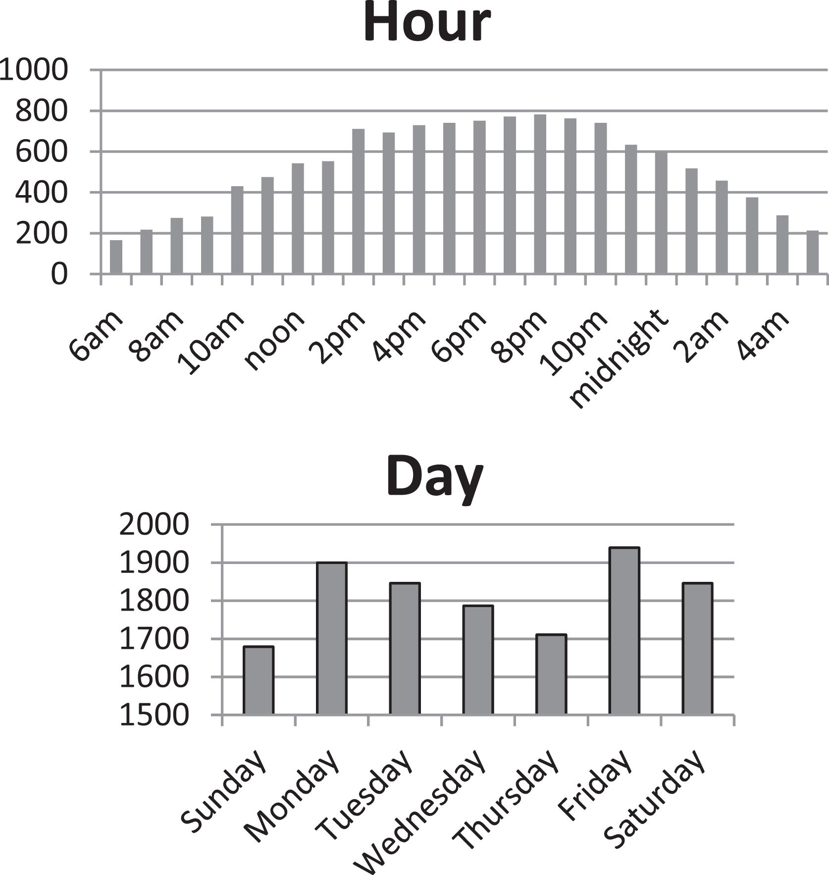
Robberies by time of day and by day of week.
The lower panel of Figure 1 shows that Fridays have most robberies and Sundays least, but it is also clear that there is much less variation in robbery across the days of the week than across the hours of the day.
The data also include information on the offenders who were arrested for committing these street robberies, including gender, racial and ethnic background, age, and residential address at the time of the robbery. The addresses were also geocoded and assigned to census blocks. The mean age was 23.9 years (SD = 8.8), 89.7 percent were male, 78.4 percent were African American, 15.6 percent were Hispanic, and 5.5 percent were White. The data did not allow us to identify offenders across multiple robberies.
Census Blocks
In addition, we collected detailed information on land use, population, and activities in all 24,594 census blocks of the city of Chicago in the year 2000. The blocks had a median size of 19,680 m2 (approximately 140 × 140 m), and there were 5,867 blocks without a residential function. These blocks include parkways, parks, beaches, cemeteries, factories, and other areas that may be surrounded by populated blocks. As robberies can be committed anywhere in outdoor public space, all census blocks are included in the analyses.
Table 1 provides descriptive statistics of the variables collected to measure the attractiveness of census blocks for street robbery and of the robbery count itself. The table shows first the percentage of nonzero values (e.g., percentage of blocks with at least one restaurant or with at least one gas station), the mean number of robberies, its standard deviation, and the minimum and maximum values observed in the data. Regarding robbery incidents, 28 percent of the blocks experienced one or more robberies, and the mean number of robberies equals .75 with a maximum of 40 robberies per block.
Descriptive Statistics Census Block Variables.a
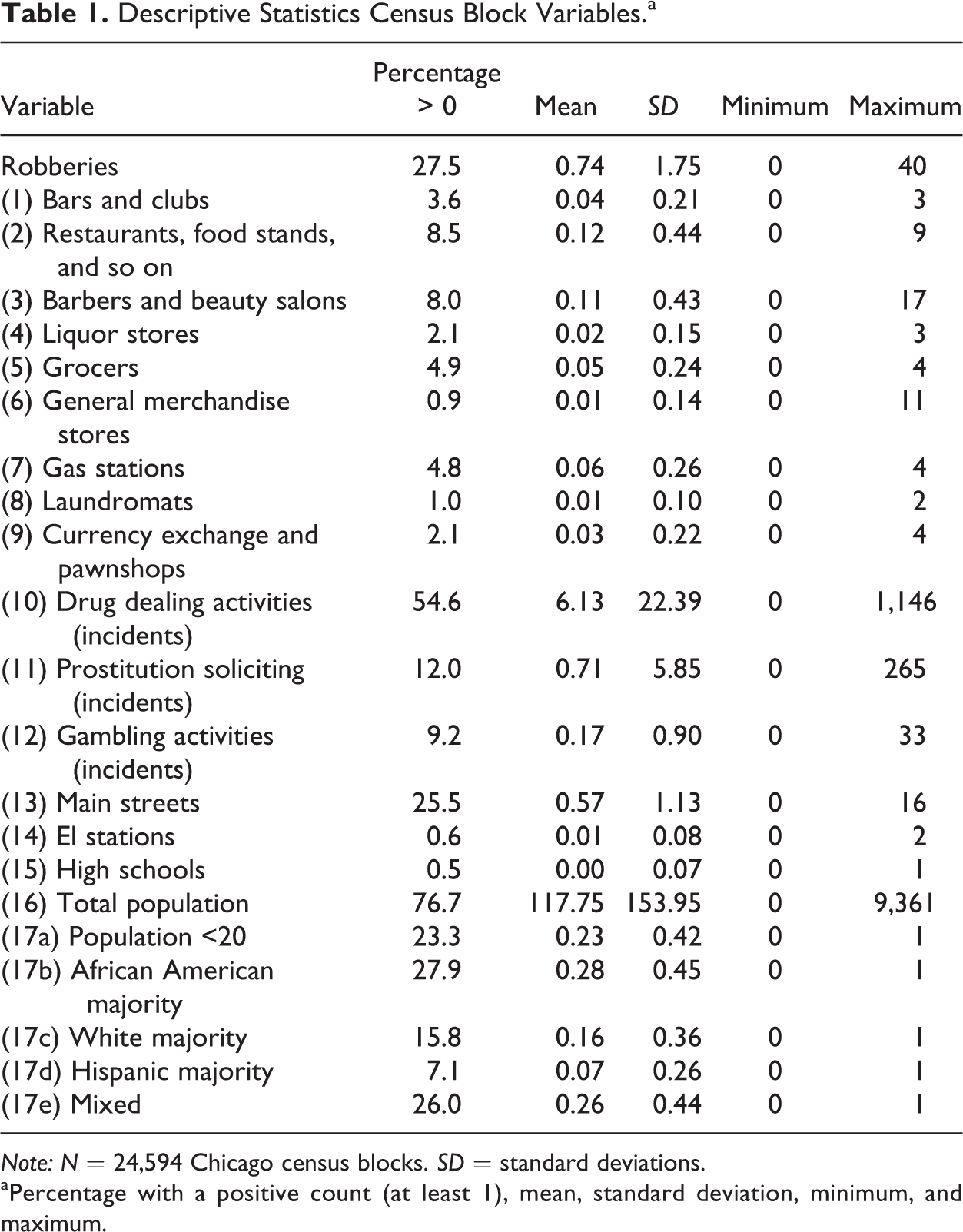
Note: N = 24,594 Chicago census blocks. SD = standard deviations.
aPercentage with a positive count (at least 1), mean, standard deviation, minimum, and maximum.
To measure small-scale retail activities in the block, we used marketing information collected by Claritas (now part of marketing research firm Nielsen) on businesses in the city of Chicago during the same period the crime data were recorded. A subset of nine types of shops and businesses with less than 11 employees was selected for which the proportion of cash transactions is likely to be high during the period between 1996 and 1998, a time during which debit card payment was uncommon and payments would typically involve either cash money or credit cards. 3 Note that the data include street robberies only. Therefore, not the businesses themselves but their customers and other people on the street are the potential robbery targets. The selected businesses include (1) bars and clubs; (2) restaurants, fast-food outlets, and food stands; (3) barber shops and beauty salons; (4) liquor stores; (5) grocery stores; (6) general merchandise shops; (7) gas stations; (8) laundromats; and (9) pawnshops, currency exchange, and check-cashing services. All nine categories are mutually exclusive, so that each store or business is counted in only a single category. Unfortunately, the business data did not include information on opening and closing hours and days. This implies that it is not precisely known when they had been open and thus served as a potentially criminogenic environment.
To measure the local presence of illegal retail activities, in particular drugs dealing, prostitution, and illegal gambling, geocoded incident files of the Chicago Police Department of the years 1996 to 1998 were aggregated to the census block level. The variables measure numbers of (10) drug-related incidents, which are arrests for soliciting or selling drugs; (11) prostitution-related incidents, which are arrests for soliciting paid sexual services by prostitutes or their customers; and (12) gambling-related incidents, which are arrests for organizing or participating in illegal gambling. These three types of illegal activities can take place on the streets, in public buildings, or private residences.
The accessibility of a block was measured by two indicator variables, namely, (13) whether the block is located along at least one main street (rather than only minor streets) and (14) whether the block contains a station of the El, the Chicago elevated railway system (also known as "L"). Data on (15) the presence of private and public high schools in a census block were based on lists compiled by the Chicago Public Schools.
Data on block population was obtained from the U.S. 2000 Census. It included (16) the total number of residents in the census block and (17) the racial and ethnic composition of the population. The information on the racial and ethnic composition was combined with the racial/ethnic background of the offender to create a dummy variable which indicates whether the majority of the census block population was of the same racial/ethnic background (African American, Hispanic, or White) as the offender. The majority threshold was defined as 75 percent. 4
Euclidian distances were calculated between the homes of the offenders and the midpoints of each of the 24,594 census blocks. Although some recent research in environmental criminology used street-network distance (or travel time) as a measures of distance (e.g., Xu and Griffiths 2016), Chicago has few natural or man-made barriers to mobility and street network distance is very strongly correlated with Euclidian distance.
The distances between offender homes and robbery locations within their own census block of residence was approximated by half the square root of the census block surface, which is about the average distance between two random points in a rectangle of the same size as the block surface (see Ghosh 1951). The home-crime distance follows a typical distance decay distribution with a long tail, indicating that the majority of home-crime trips were short and very few were long. Because the shape of the distance decay function suggests that a location’s attractiveness is a (negative) exponential function of distance from home, to linearize it, (18) the negative value of the log of distance was included in the model.
Method
In line with prior crime location choice studies (e.g., Baudains et al. 2013; Bernasco and Block 2009; Bernasco and Kooistra 2010; Bernasco and Nieuwbeerta 2005; Clare et al. 2009; Johnson and Summers 2015; Townsley et al. 2015; Vandeviver et al. 2015), the conditional logit model was used to estimate the effects of census block attributes on the probability of the census block being selected for robbery. This is a discrete choice model that is consistent with random utility maximization theory. Applied to robbery location choice, it assumes that from a set of alternative census blocks, an offender chooses to commit a robbery in the census block that, when chosen, provides them more utility than any other alternative would have. The systematic part of utility is a weighted sum of the attributes of the location, in this particular case of the 18 variables discussed in the Data section. The aim of the model estimation is to determine the values of these weights.
To explore temporal differences in location preference, 12 models were estimated separately for each of 12 two-hour blocks (4–6 a.m., 6–8 a.m., 8–10 a.m., etc.) and 7 models were estimated separately for each of the seven days of the week. The choice for two-hour blocks seemed like a reasonable compromise between the need to use a fine-grained temporal measure on the one hand, and the need for statistical power in modeling and efficiency in presenting results on the other hand. A choice in favor of one-hour blocks was considered but would have implied twice as many models to be estimated and presented. 5
Both Bernasco and Block (2011) and Haberman and Ratcliffe (2015) found spatially lagged (spillover) effects to be significant, meaning that factors present in a census block not only affect the robbery risk locally but also influence robbery risk in adjacent census blocks. We did consider the inclusion of lagged effects in the analysis but decided against it. One reason was that including them would have doubled the already quite large number of model estimates. Another reason was that the results of the two aforementioned studies demonstrate that the main effects of crime attractors are typically much larger than their spatially lagged effects. These arguments made us decide that we better use computer resources and statistical power to distinguish between time periods than add another layer of spatial complexity.
Like other crime location choice studies that used many small spatial units of analysis (Bernasco et al. 2013; Vandeviver et al. 2015), to reduce the size of the estimation problem, we used a sampling of alternatives technique (McFadden 1978). This technique has also been applied for other spatial choice problems, such as the migrant’s choice of residential location (Duncombe, Robbins, and Wolf 2001), the angler’s choice of a fishing site (Feather 1994), the traveler’s choice of a route (Frejinger, Bierlaire, and Ben-Akiva 2009), the worker’s choice of employment location (Kim et al. 2008), and the consumer choice of local telephone service (Train, McFadden, and Ben-Akiva 1987). For each robbery, the chosen census block and a sample of the other 24,593 census blocks were included in the analysis (thereby ignoring information about the census blocks not included in the sample). The sample sizes were chosen to maximally use the computer’s memory resources. For the analysis of daily variation (12 models), the sample size was 11,999 census blocks, and for the analysis of weekly variation (seven models), the sample size was 7,999 census blocks.
Bootstrap Estimates
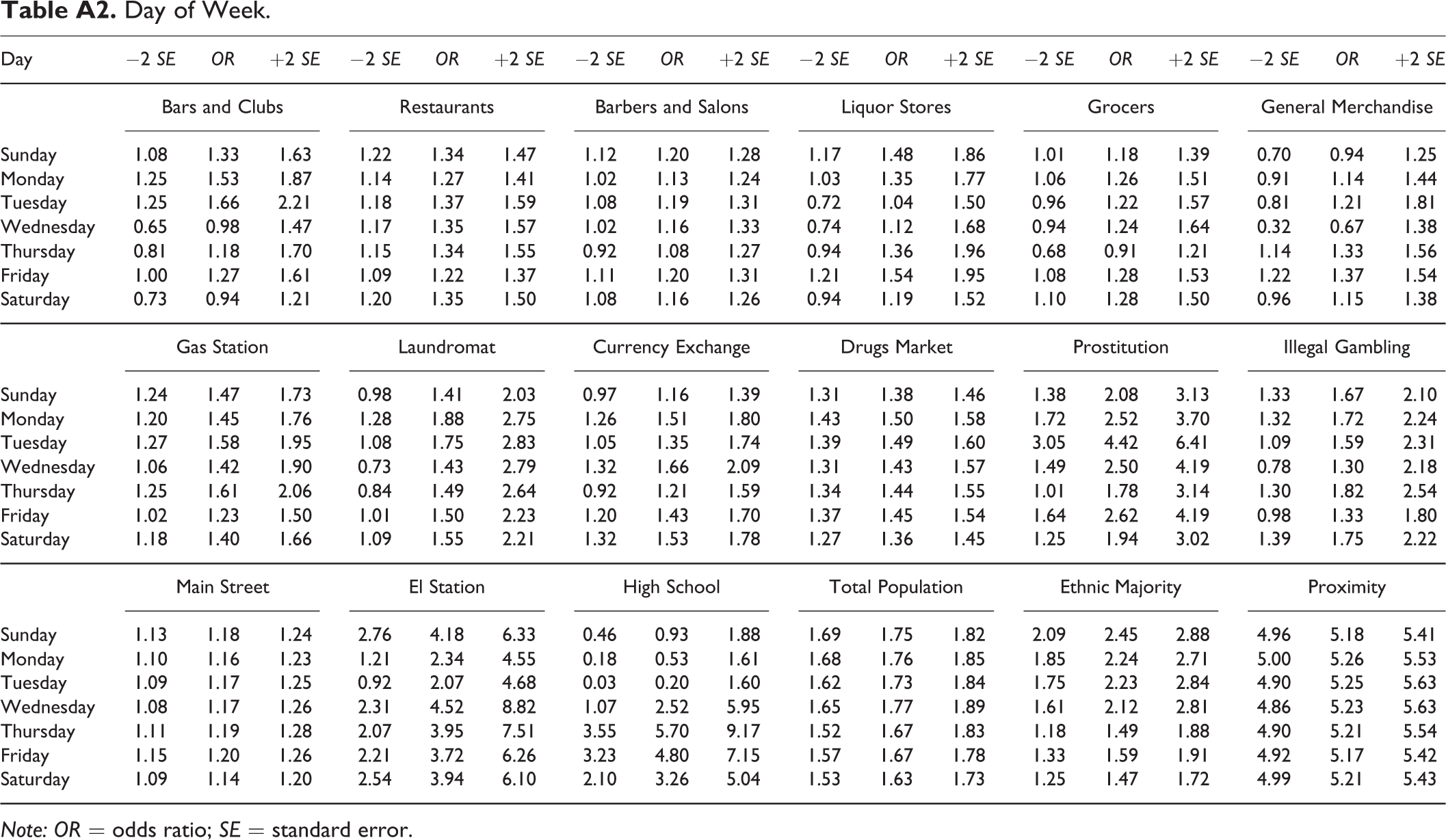
To obtain robust estimates, the analysis just described was repeated 10 times, each time selecting a different random sample of 11,999 (daily variation) or 7,999 (weekly variation) alternative census blocks. Because this bootstrapping technique yields an additional (between iteration) variance in the parameter estimates, it provides a more precise estimate of the parameters and a more conservative estimate of their standard errors. To combine the results of the 10 iterations, we used Rubin’s (1987) formulae for combining the estimates of bootstrapped multiple regression analyses. To sum up, the complete estimation procedure involved the following steps: From the 12,938 robberies, determine the time and day. Select all robberies that fall within a specific time slot (1 of the 12 two-hour time slots or one for each of the seven days of the week separately). Based on (Bernasco 2006) the supplementary material of Bernasco et al. (2013) and note 2 of this article, for each of the selected robberies involving multiple offenders, select a random offender from those involved. For each of these robberies, select the block where the robbery was actually perpetrated and add to this a random sample of 11,999 or 7,999 blocks of the other 24,593 census blocks. Estimate the model and save the estimated coefficients and their robust standard errors. Repeat steps 1 through 4 for 10 times, each time taking another time/day slot and different random samples of blocks and collecting the regression coefficients and their standard errors at each step. Using Rubin’s rules for combining regression coefficients and standard errors from bootstrapped estimation results for each variable, combine the 10 coefficient estimates and corresponding standard error estimates into an overall coefficient estimate and an overall standard error estimate. These are reported graphically in Figures 2 and 3 and ad verbatim in Appendix Table A1 (time of day) and Appendix Table A2 (day of week). Briefly, Rubin’s rules state that the overall coefficient is the average coefficient across iterations, while the overall standard error is the square root of the summed within-iteration and between-iteration variances.
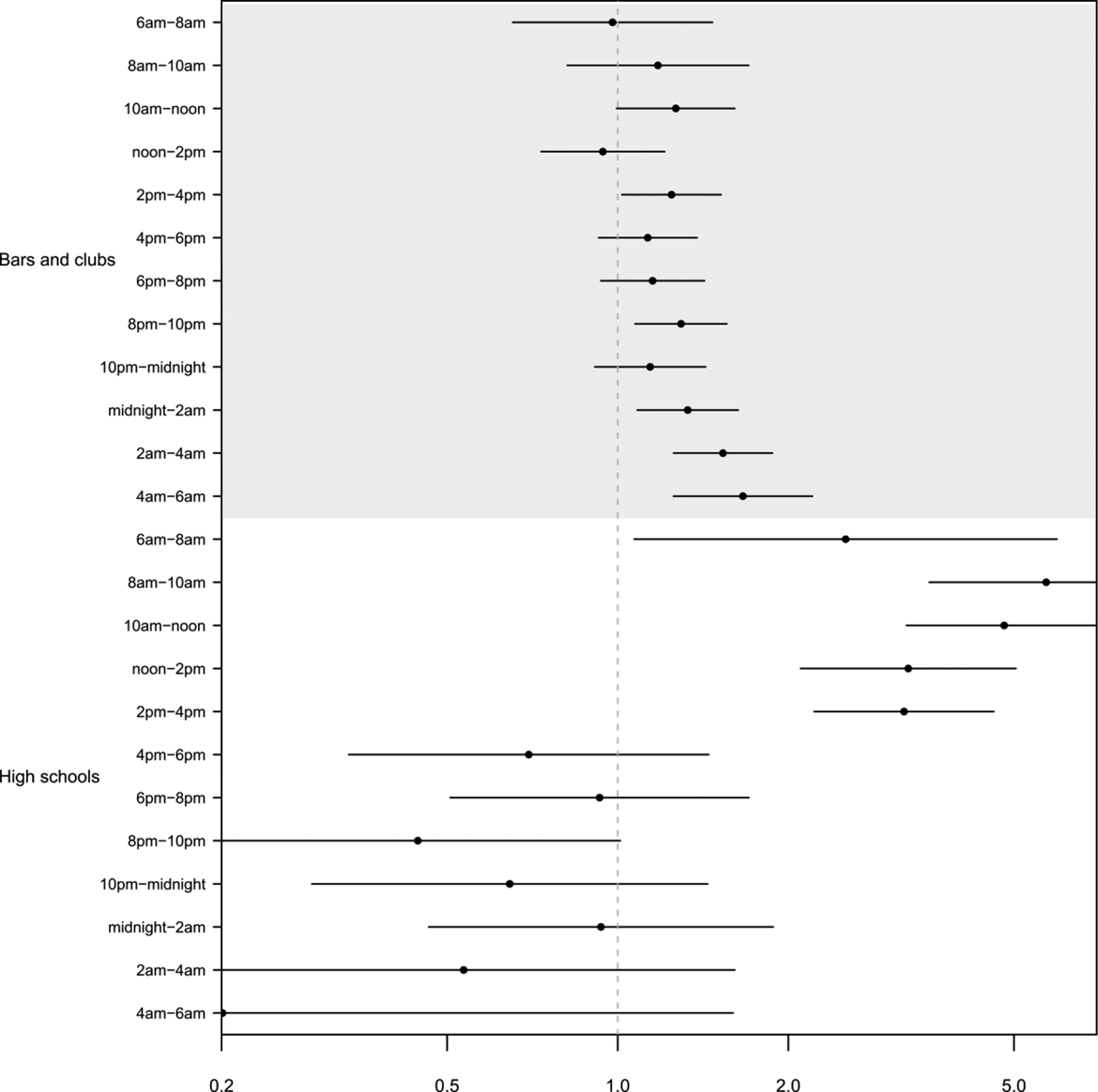
Time of the day, model estimates (odds ratios), and 95 percent confidence intervals for bars and clubs and for high schools.
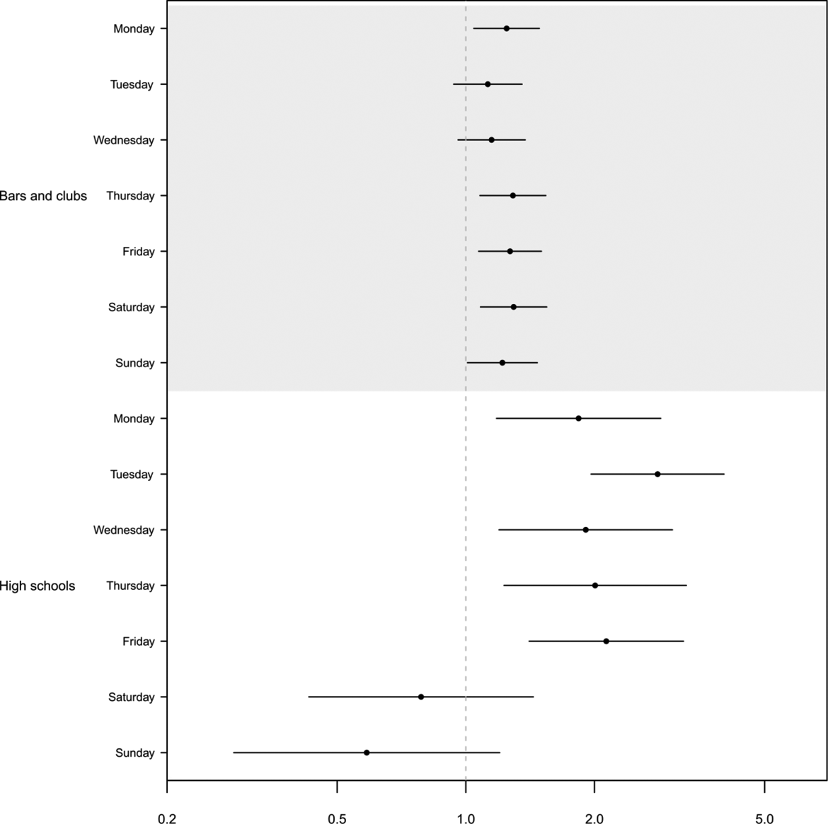
Day of the week, model estimates (odds ratios), and 95 percent confidence intervals for bars and clubs and for high schools.
Findings
Estimating 19 models (12 time slots and 7 days) with 18 independent variables per model produces no less than 342 coefficients and as many standard errors. 6 To organize the main results of the analysis, the estimated coefficients (odds ratios) and their 95 percent confidence intervals are visualized Figure 2 (variation across the hours of the day) and Figure 3 (variation across the days of the week). To save space, these figures include the results for only two of the 18 independent variables, namely, numbers of bars and clubs and high schools. All point estimates and their 95 percent confidence intervals are reported in Appendix Table A1 (time of day) and Appendix Table A2 (day of week) and are sufficient to reproduce the figures for each of the 18 facilities. 7
Time of Day
In each graph, the horizontal axis shows the estimated odds ratio on a logarithmic scale ranging from .2 to 5 with midpoint 1. All points left of the midpoint have odds ratios between .2 and 1 and represent negative effects. All points located right of the midpoint have odds ratio between 1 and 5 and represent positive effects.
To illustrate the organization of the graphs, we discuss the top panel of Figure 2, labeled “bars and clubs.” Just right from the vertical axis are the descriptions of the 12 time slots (6–8 a.m., 8–10 a.m., 10 a.m.–noon, noon–2 p.m., 2–4 p.m., 4–6 p.m., 6–8 p.m., 8–10 p.m., 10–midnight, midnight–2 a.m., 2–4 a.m., and 4–6 a.m.). Further to the right are solid horizontal lines with dots in the middle. The dots represent the estimated odds ratios. The horizontal lines are the 95 percent confidence intervals of the estimates. Thus, the length of the lines left and right of the dots represent twice the standard error on both sides. For example, the top line of the panel labeled “6–8 a.m.” applies to the period between 6 and 8 in the morning. The dot, an estimated odds ratio of .98, is just below 1 and therefore slightly negative. As the 95 percent confidence interval ranges between .65 and 1.47 and thus includes the value of 1, this is not a statistically significant effect and therefore it cannot be concluded that between 6 and 8 in the morning, street robbers are more likely to target census blocks where bars and clubs are located than to target other blocks. During the three time slots near the bottom of the panel between midnight and 6 a.m., however, the 95 percent confidence intervals are located completely right of the midpoint. Thus, during this period, blocks with bars or clubs are significantly more likely to be targeted than blocks without bars or clubs.
Whether the robbery location preferences vary by time of day and day of the week, we test by comparing the different odds ratios and associated confidence intervals. Two odds ratios are statistically significantly different if their 95 percent confidence intervals have no overlap. In Figure 2, it can be seen that the effect of bars and clubs in period noon–2 p.m. is significantly lower than their effects in periods 2–4 a.m. and 4–6 a.m., but that all other possible pairs do not differ statistically significantly.
Appendix Table A1 contains point estimates and confidence intervals of the odds ratios regarding the following other retail businesses: restaurants and fast-food outlets, barber shops and beauty salons, liquor stores, grocery stores, general merchandise stores, gas stations, laundromats, and pawnshops and cash services. The presence of restaurants and fast-food outlets has a positive effect on street robbery during all periods of the day, ranging from a low odds ratio of 1.15 between 4 p.m. and 6 p.m. to a maximum of 1.37 between 4 a.m. and 6 a.m. More important for the main research question, however, is that all 95 percent confidence intervals overlap with each other, so that none of the differences in odds ratios between time periods is statistically significant. In other words, robbers’ preference for blocks with restaurants and fast-food outlets remains stable throughout the entire day.
A similar pattern of significant positive effects with little variation over the day was established for the presence of barbershops and beauty salons. In only a single time period (8–10 a.m.) was their presence not statistically significantly positive. Again, however, there are hardly any differences between the 12 time periods: Blocks with barbershops and beauty salons appear to attract street robbers even at odd hours, such as in the late evening or during the night.
The effects of the presence of liquor stores on street robberies in census blocks are all positive and appear to vary substantially (odds ratio between 1.04 and 1.54), but their 95 percent confidence bands are too wide to make definite statements about effect variability. Still, even if differences would have been larger and confidence bands tighter, the irregular temporal pattern does not seem to match with activity levels around liquor stores.
The other retail businesses are grocery stores, general merchandise stores, gas stations, laundromats, and pawnshops and cash services. All show effects very similar to those found for the four business types discussed above: their presence attracts robbery, their effects are often though not always statistically significant, but their variation across the day is quite limited and almost completely within the 95 percent confidence intervals around the estimates of the other two-hour time blocks. The same conclusion is drawn regarding the presence of illegal markets for drugs, sexual services and gambling, measures of blocks accessibility (presence of El stations and main streets along the block), total population, and distance from home.
Although the confidence intervals of most two-hour blocks overlap, indicating their differences are not statistically significant, some slight temporal variability appears to exist in robbers’ preference to select blocks where their own racial or ethnic group is a majority: They seem to prefer blocks with in-group majorities more during evenings and late nights than during mornings and afternoons.
The single notable exception to the general pattern is found for high schools as is clear from Figure 2. In fact, of the 18 variables, the presence of a high school in a block is the only one that displays a strong temporal variation in location preference. During school hours in the morning and early afternoon (i.e., from 6 a.m. to 4 p.m.), the effects are statistically significantly positive, but outside these hours they are all (nonsignificantly) negative. This suggests that high school students are vulnerable robbery victims who cluster temporally during school hours only and might also be an indication that some or most of the street robberies in blocks with high schools are also perpetrated by students of these high schools.
In sum, the large majority of reported effects are positive and statistically significant, confirming prior conclusions about the attractiveness of cash economies, illegal markets, and accessibility to street robbers (Bernasco and Block 2009, 2011; Bernasco et al. 2013; Haberman and Ratcliffe 2015). A slightly closer look, however, reveals that except for those of high schools, these forces of attraction do not seem to vary over the hours of the day in a meaningful and statistically significant way at all.
Day of Week
Analogous to Figure 2, Figure 3 graphically displays coefficient variations across the seven days of the week again with respect to bars and clubs and high schools. The findings on the 16 other census block characteristics are documented in Appendix Table A2. Overall, the results mirror those on daily variation: Most coefficients are positive, large differences between the days of the week are almost absent, and where they exist they do not reach acceptable levels of statistical significance. For example, census blocks with bars and clubs attract robbers during most days of the week (although on Tuesdays and Wednesdays, the effects are not statistically significant), but the estimated odds ratios only vary between 1.13 on Tuesdays and 1.29 on Thursdays and Saturdays, and the differences across the seven coefficients are statistically nonsignificant. With slight variations, similar results are found for almost all variables: Most effects of facilities are positive and significant during most days of the week, but they do not differ statistically significantly across the days of the week.
High schools are clearly again the exception, as with respect to the weekly cycle, we see that during weekends when schools are vacant, census blocks with high schools are not the attractive robbery places they are during regular weekdays when the schools are operational.
Discussion
Although the frequency of street robberies varies widely over the course of the day and somewhat across the days of the week, our findings suggest that the location preferences of robbers are mostly stable over time. The findings thus confirm that street robbers prefer to attack near cash-intensive businesses and other places that seem to promise high benefits and low risks. However, they also demonstrate that robbers prefer these places even when the businesses are closed and when activity levels are therefore low. The same holds true for illegal markets and transit facilities. They do attract robbery, but they do so throughout the day without much hour-to-hour variation. They also attract robbery throughout the week without much day-to-day variation. High schools are a notable exception, as they appear to be only attractive places for robbery around school hours but not in evenings and nights nor during weekends. These results are largely in line with those of Haberman and Ratcliffe (2015), who identified a few temporal differences in location preferences, but who also concluded that many location preferences do not appear to vary in line with theoretical expectations.
The main hypothesis of Haberman and Ratcliffe and of ourselves was, however, that the effects of most potential target block attributes would systematically vary over the course of the day and the week, because we know that these attributes have daily and weekly activity cycles. During the night, schools, grocery shops, and El stations are simply not attracting any potential victims that could be robbed.
The rejection of the hypothesis seems to challenge the view that street robbers select utility-maximizing locations for committing robberies. At first sight, it also appears to contradict the routine activity assertion that robberies peak where and when many offenders and victims converge in time and space: Many of the facilities appear to attract robbers at times of the day during which they are unlikely to attract any customers at all, such as bars and clubs at 10 a.m.–noon or barber shops and beauty salons between midnight and 6 a.m.
How can we explain that street robbers seem to mostly ignore daily rhythms of potential victims when they select target areas? For example, how can we explain that they prefer blocks with grocers between 2 a.m. and 4 a.m., when the grocers are likely to be closed?
One possible explanation for these findings is model misspecification. We may have missed some facilities or block features that are important for robbery location choice, in particular, if the presence of these facilities or features correlates with the presence of other facilities or features that have different time cycles. We did, for example, not have information on the presence of ATMs that operate 24/7. Haberman and Ratcliffe (2015) show that ATMs are indeed attractive for robbers all day. If ATMs are located near grocery stores with limited opening times, then they will create bias in the grocery store estimates because our results make it look like the grocery stores attract robberies at odd hours, while in fact the ATMs do. In addition to ATMs, other facilities not included in our data are banks, drug treatment centers, neighborhood parks, and public housing communities (Haberman and Ratcliffe 2015), some of which might be correlated spatially but not temporally with the facilities used in our analysis. However, because Haberman and Ratcliffe (2015) also find limited time variability in the attractiveness of facilities while controlling for the presence of ATMs and the other facilities not included in our data, we believe that our findings are not the result of omitted variable bias.
Another possible reason for street robbers ignoring the daily rhythms of potential victims is that potential victims and their guardians are the same persons (Block and Block 1999). For most nonconfrontational property crimes, the presence of potential targets does not continuously coincide with the presence of potential guardians. Burglary targets (houses and apartments) stay in place but their residents leave, typically during daytime. For street robbers, however, people on the street are both potential victims and guardians of other potential victims, and therefore numbers of potential victims and guardians are always in balance. Still, this observation does not help us explain why robbers are more likely to attack near retail businesses and other cash intensive facilities far beyond the opening hours of these facilities.
An alternative explanation is that street robbery is generally not a premeditated activity, but an impulsive decision driven by opportunities that offenders are exposed to during their legitimate routine activities. The findings might well be consistent with routine activity, which states that crime takes place where and when motivated offenders and suitable and unguarded victims converge. If offenders spend large amounts of their outdoors routine activities in or around cash economies, illegal markets, transit facilities, or schools, these are the places where they may occasionally encounter opportunities or provocations that motivate them to commit street robberies. In other words, if robbers are not very mobile themselves, their crimes will always be perpetrated in the same places irrespective of the density of potential targets at particular times of the day or day of the week.
The combination of our own findings and those of Haberman and Ratcliffe (2015) tentatively suggest that the hypothesis of temporal variation in street robbery location preferences may be wrong. Except for the environs of high schools, which appear not to attract robbers when they are closed, the attraction of cash economies, illegal markets, and other businesses and facilities appears to be much more stable over the hours of the day and over the days of the week than various theoretical frameworks make us expect.
Human routine activity patterns not only follow daily and weekly cycles but also annual cycles. Annual cycles in routine activities are often related to climatological conditions, including temperature, precipitation, and daylight hours. Andresen and Malleson (2013) tested whether spatial patterns of many types of crime (assault, burglary, robbery, sexual assault, theft, theft from vehicle, and theft of vehicle) varied between winter, spring, summer, and fall in Vancouver, Canada. In line with our own results regarding daily and weekly cycles, they concluded that robbery “appears to occur in the same places regardless of the season of year” (Andresen and Malleson 2013:31).
An important caveat of the present analysis is that time (hours, days) is used as a proxy measure for the physical presence of other people and for the tangible circumstance that a certain shop or business is actually open. We did not actually measure each business’ opening hours, measure the average number of people present per census block per time slot, or count numbers of vulnerable people on the streets. Future research in this area should be able to take advantage of the increasing availability of unobtrusive and automatically collected georeferenced measures of human presence through contemporary developments in information and communication technologies, including smartphones and other location services, and social media (Malleson and Andresen 2014; Raento, Oulasvirta, and Eagle 2009).
Footnotes
Appendix
Day of Week.
| Day | −2 SE | OR | +2 SE | −2 SE | OR | +2 SE | −2 SE | OR | +2 SE | −2 SE | OR | +2 SE | −2 SE | OR | +2 SE | −2 SE | OR | +2 SE |
|---|---|---|---|---|---|---|---|---|---|---|---|---|---|---|---|---|---|---|
| Bars and Clubs | Restaurants | Barbers and Salons | Liquor Stores | Grocers | General Merchandise | |||||||||||||
| Sunday | 1.08 | 1.33 | 1.63 | 1.22 | 1.34 | 1.47 | 1.12 | 1.20 | 1.28 | 1.17 | 1.48 | 1.86 | 1.01 | 1.18 | 1.39 | 0.70 | 0.94 | 1.25 |
| Monday | 1.25 | 1.53 | 1.87 | 1.14 | 1.27 | 1.41 | 1.02 | 1.13 | 1.24 | 1.03 | 1.35 | 1.77 | 1.06 | 1.26 | 1.51 | 0.91 | 1.14 | 1.44 |
| Tuesday | 1.25 | 1.66 | 2.21 | 1.18 | 1.37 | 1.59 | 1.08 | 1.19 | 1.31 | 0.72 | 1.04 | 1.50 | 0.96 | 1.22 | 1.57 | 0.81 | 1.21 | 1.81 |
| Wednesday | 0.65 | 0.98 | 1.47 | 1.17 | 1.35 | 1.57 | 1.02 | 1.16 | 1.33 | 0.74 | 1.12 | 1.68 | 0.94 | 1.24 | 1.64 | 0.32 | 0.67 | 1.38 |
| Thursday | 0.81 | 1.18 | 1.70 | 1.15 | 1.34 | 1.55 | 0.92 | 1.08 | 1.27 | 0.94 | 1.36 | 1.96 | 0.68 | 0.91 | 1.21 | 1.14 | 1.33 | 1.56 |
| Friday | 1.00 | 1.27 | 1.61 | 1.09 | 1.22 | 1.37 | 1.11 | 1.20 | 1.31 | 1.21 | 1.54 | 1.95 | 1.08 | 1.28 | 1.53 | 1.22 | 1.37 | 1.54 |
| Saturday | 0.73 | 0.94 | 1.21 | 1.20 | 1.35 | 1.50 | 1.08 | 1.16 | 1.26 | 0.94 | 1.19 | 1.52 | 1.10 | 1.28 | 1.50 | 0.96 | 1.15 | 1.38 |
| Gas Station | Laundromat | Currency Exchange | Drugs Market | Prostitution | Illegal Gambling | |||||||||||||
| Sunday | 1.24 | 1.47 | 1.73 | 0.98 | 1.41 | 2.03 | 0.97 | 1.16 | 1.39 | 1.31 | 1.38 | 1.46 | 1.38 | 2.08 | 3.13 | 1.33 | 1.67 | 2.10 |
| Monday | 1.20 | 1.45 | 1.76 | 1.28 | 1.88 | 2.75 | 1.26 | 1.51 | 1.80 | 1.43 | 1.50 | 1.58 | 1.72 | 2.52 | 3.70 | 1.32 | 1.72 | 2.24 |
| Tuesday | 1.27 | 1.58 | 1.95 | 1.08 | 1.75 | 2.83 | 1.05 | 1.35 | 1.74 | 1.39 | 1.49 | 1.60 | 3.05 | 4.42 | 6.41 | 1.09 | 1.59 | 2.31 |
| Wednesday | 1.06 | 1.42 | 1.90 | 0.73 | 1.43 | 2.79 | 1.32 | 1.66 | 2.09 | 1.31 | 1.43 | 1.57 | 1.49 | 2.50 | 4.19 | 0.78 | 1.30 | 2.18 |
| Thursday | 1.25 | 1.61 | 2.06 | 0.84 | 1.49 | 2.64 | 0.92 | 1.21 | 1.59 | 1.34 | 1.44 | 1.55 | 1.01 | 1.78 | 3.14 | 1.30 | 1.82 | 2.54 |
| Friday | 1.02 | 1.23 | 1.50 | 1.01 | 1.50 | 2.23 | 1.20 | 1.43 | 1.70 | 1.37 | 1.45 | 1.54 | 1.64 | 2.62 | 4.19 | 0.98 | 1.33 | 1.80 |
| Saturday | 1.18 | 1.40 | 1.66 | 1.09 | 1.55 | 2.21 | 1.32 | 1.53 | 1.78 | 1.27 | 1.36 | 1.45 | 1.25 | 1.94 | 3.02 | 1.39 | 1.75 | 2.22 |
| Main Street | El Station | High School | Total Population | Ethnic Majority | Proximity | |||||||||||||
| Sunday | 1.13 | 1.18 | 1.24 | 2.76 | 4.18 | 6.33 | 0.46 | 0.93 | 1.88 | 1.69 | 1.75 | 1.82 | 2.09 | 2.45 | 2.88 | 4.96 | 5.18 | 5.41 |
| Monday | 1.10 | 1.16 | 1.23 | 1.21 | 2.34 | 4.55 | 0.18 | 0.53 | 1.61 | 1.68 | 1.76 | 1.85 | 1.85 | 2.24 | 2.71 | 5.00 | 5.26 | 5.53 |
| Tuesday | 1.09 | 1.17 | 1.25 | 0.92 | 2.07 | 4.68 | 0.03 | 0.20 | 1.60 | 1.62 | 1.73 | 1.84 | 1.75 | 2.23 | 2.84 | 4.90 | 5.25 | 5.63 |
| Wednesday | 1.08 | 1.17 | 1.26 | 2.31 | 4.52 | 8.82 | 1.07 | 2.52 | 5.95 | 1.65 | 1.77 | 1.89 | 1.61 | 2.12 | 2.81 | 4.86 | 5.23 | 5.63 |
| Thursday | 1.11 | 1.19 | 1.28 | 2.07 | 3.95 | 7.51 | 3.55 | 5.70 | 9.17 | 1.52 | 1.67 | 1.83 | 1.18 | 1.49 | 1.88 | 4.90 | 5.21 | 5.54 |
| Friday | 1.15 | 1.20 | 1.26 | 2.21 | 3.72 | 6.26 | 3.23 | 4.80 | 7.15 | 1.57 | 1.67 | 1.78 | 1.33 | 1.59 | 1.91 | 4.92 | 5.17 | 5.42 |
| Saturday | 1.09 | 1.14 | 1.20 | 2.54 | 3.94 | 6.10 | 2.10 | 3.26 | 5.04 | 1.53 | 1.63 | 1.73 | 1.25 | 1.47 | 1.72 | 4.99 | 5.21 | 5.43 |
Note: OR = odds ratio; SE = standard error.
Acknowledgments
We thank the editor of JRCD and three anonymous reviewers for stimulating comments that helped us to improve this article.
Declaration of Conflicting Interests
The author(s) declared no potential conflicts of interest with respect to the research, authorship, and/or publication of this article.
Funding
The author(s) disclosed receipt of the following financial support for the research, authorship, and/or publication of this article: Stijn Ruiter’s contribution to this study was funded by the Netherlands Organization for Scientific Research Innovational Research Incentives Scheme Vidi [452-12-004].