Sage Journals: Discover world-class research

Abstract

Existing models for predicting conflict fatalities frequently produce conservative forecasts that gravitate towards the mean. While these approaches have a low average prediction error, they offer limited insights into temporal variations in conflict-related fatalities. Yet, accounting for variability is particularly relevant for policymakers, providing an indication on when to intervene. In this article, we introduce a novel risk-taking methodology, the ‘Shape finder’, designed to capture variability in fatality data, or rather the sudden surges and declines in the number of deaths over time. The method involves isolating historically analogous sequences of fatalities to create a reference repository. Comparing the shape of the input sequence to the historical references, the most similar historical cases are selected. Predictions are then generated using the average future outcomes of the selected matches. The Shape finder is derived from the theoretical understanding that strategic and adaptive interactions between the government and a non-state armed group produce recurring temporal patterns in fatality data, which are indicative of broader developments. In this article, we demonstrate that our approach maintains high accuracy while significantly enhancing the ability to predict shifts, surges, and declines in conflict fatalities over time. We show that combining the Shape finder with existing approaches, the Violence Early-Warning System ensemble, achieves a lower mean squared error and better accounts for variability in fatality data. The Shape finder methodology performs particularly well for high intensity cases, or rather country-months with substantial armed violence.

Keywords

Armed conflict dynamic time warping pattern recognition prediction temporal patterns time series

Conflict forecasting has emerged as an important subfield of armed conflict studies (e.g. Hegre et al., 2021; Mueller and Rauh, 2022). Recent advances have harnessed numerous data sources, from geopolitical indicators to digital media, as well as methods from statistics, machine learning, and game theory. Models such as the Violence Early-Warning System (VIEWS), for example, have set benchmarks by integrating complex datasets, including event data and socio-economic indicators, to forecast conflict occurrences and intensities on both national and subnational levels (Hegre et al., 2019, 2021). By analysing past conflict patterns and integrating various geopolitical, socio-economic, and event-based data, forecasts help identify underlying trends and potential triggers for armed conflict.

Despite these advancements, most models rely on static, cross-sectional data that inadequately address the non-linear and evolving nature of conflicts. As a result, these forecasts, while generally accurate over broad time scales, fail to capture critical short-term fluctuations and sudden escalations. Such shortcomings are significant, as understanding these temporal variations is crucial for effective conflict mitigation and response strategies. The inability to anticipate these rapid changes can lead to missed opportunities for timely interventions and appropriate allocation of resources (Mueller and Rauh, 2022).

To address these limitations, this article introduces the ‘Shape finder’, designed to enhance the predictive accuracy of conflict-related fatalities by focusing on the temporal sequences and patterns in data. The main goal is to capture variability, rather than producing overly conservative – flat – predictions around the mean. Variability refers to the short-term escalation and de-escalation in the number of fatalities over time. The Shape finder methodology distinguishes itself by using Dynamic Time Warping (DTW) to compare sequences of casualties across different contexts and time periods. This method allows us to align sequences of varying lengths and scales, making it possible to identify analogous patterns across disparate datasets. By focusing on sequences rather than isolated data points, the Shape finder predicts potential escalations and de-escalations in fatality data with greater precision, instead of returning flat forecasts.

Empirical tests of the Shape finder demonstrate its robust performance when compared to three baselines – the null model, the $t - 1$ model, and the VIEWS ensemble. The Shape finder not only predicts the occurrence and intensity of conflict-related fatalities with a comparable degree of accuracy to existing models, but also better captures temporal variability – an area where existing models fall short. Existing models tend to overlook short-term fluctuations and sudden escalations, focusing instead on broader trends – and quickly revert to the mean. In contrast, the Shape finder can detect and forecast critical changes ahead of time.

In addition, we construct a compound model that combines the Shape finder and VIEWS, selecting risk-taking and risk-averse approaches depending on our level of confidence in the predictions. The compound performs better than the constituent models in terms of both prediction error and the ability to capture variability in fatality data. The Shape finder is particularly suitable for high complexity input shapes – casualties time series with high variability – although it does tend to produce overpredictions for low complexity inputs – time series without significant variability, and therefore without meaningful ups-and-downs in the number of fatalities.

The remainder of the article is organized as follows. We first review the state of the art in conflict prediction, and we put forward our theoretical arguments. Then, we describe the data and methodologies used in this study, including a comprehensive description of the Shape finder algorithm and its implementation. Finally, we present the results of our empirical analysis and discuss the implications of our findings.

Conflict prediction

Conflict prediction has emerged as a thriving subfield of peace and conflict studies (Chadefaux, 2017; Colaresi and Mahmood, 2017; Hegre et al., 2017; Ward et al., 2010). A range of academic early-warning systems exists to forecast armed conflict, complemented by operational systems used by practitioners. Rød et al. (2024) present a comparative review.

Among these systems, the Violence Early-Warning System (VIEWS) stands out, offering monthly forecasts for the number of fatalities in state-based armed conflict on a global scale, with projections extending up to three years into the future (Hegre et al., 2019, 2021). VIEWS employs a sophisticated ensemble model that incorporates structural variables related to socio-economic, geographic and political factors. Another approach by Mueller and Rauh (2022) relies on a large text corpus from over 4 million news articles, and extracts topics using Latent Dirichlet Allocation. Those topics, in addition to a set of variables on conflict history, are used to predict the onset of organized violence per country-month. Finally, the Armed Conflict Location and Event Data Project (ACLED) predicts organized political violence up to six months ahead, mostly relying on ACLED data as predictors (ACLED, 2023). CAST forecasts are generated on a global scale, encompassing both national and sub-national levels. As the review by Rød et al. (2024) demonstrates, the models assign a high risk of violent action to a similar set of countries, regardless of the differences across these systems.

Despite advances in methodology and data collection, conflict prediction remains a challenging field. Several key issues continue to hinder progress in this area (e.g. Cederman and Weidmann, 2017). The inherent imbalance in conflict data, with peaceful periods far outnumbering instances of violence, poses significant analytical challenges. There is also an ongoing debate among scholars about the fundamental causes of armed conflict, leading to uncertainties in model specification. The quality and depth of available data often falls short of what is required for precise predictions, especially in regions prone to conflict, where data collection can be difficult or dangerous. The ‘hard problem of conflict prediction’ (Mueller and Rauh, 2022: 2442) are conflict onsets, or rather cases with no prior conflict history. These instances are particularly difficult to anticipate using structural predictors that measure economic performance, demographics, or political institutions. Finally, idiosyncratic events – ‘historical accidents’ (Cederman and Weidmann, 2017: 3) such as the end of the Cold War or Brexit – are perhaps impossible to predict.

The rarity of armed conflicts poses one of the most significant methodological challenges. Rare events occur only infrequently, which means that the dataset has a large number of zeros (King and Zeng, 2001). Indeed, it has been noted that the distribution of fatalities is extremely right-skewed. Logit regression and more complex machine learning algorithms are known to underpredict in the context of rare events (Cederman and Weidmann, 2017; King and Zeng, 2001). The right-skewed structure of conflict data encourages risk-averse predictions. For example, a conservative model that exclusively predicts zero fatalities will achieve a low mean squared error (MSE) when dealing with rare events. Consequently, most models tend to produce risk-averse predictions that effectively identify a baseline risk of conflict but struggle to detect temporal variations and sudden shifts in the data. These models produce ‘flat’ predictions close to the mean value of fatalities. We show examples in Figure 1.

Figure 1.

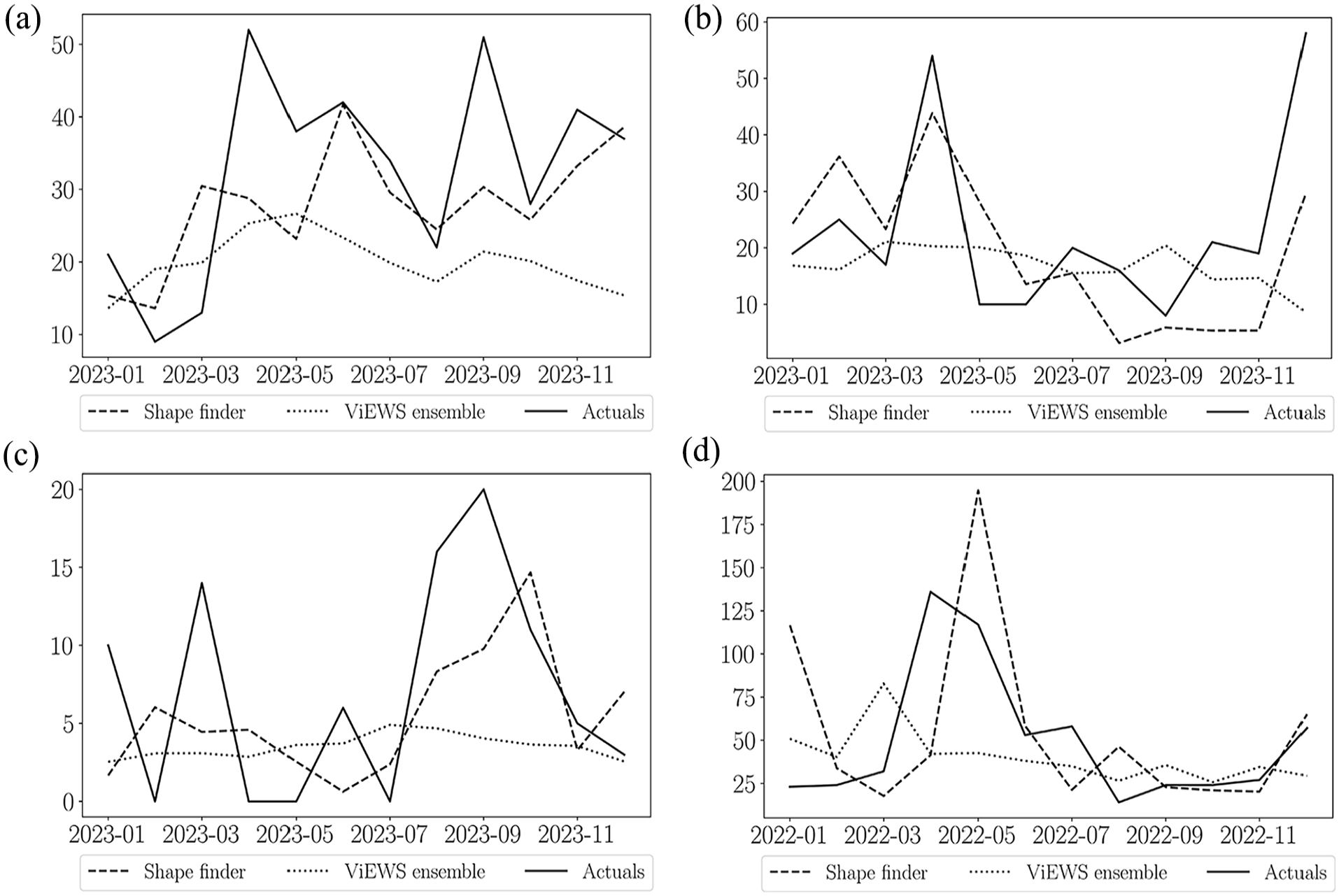
Sample predictions. The actual fatalities are shown in as solid lines, with the risk-averse model (VIEWS ensemble) in dotted lines and the risk-taking model (Shape finder) in dashed lines. The risk-averse model generates flat predictions around the mean, missing sudden surges and declines. The risk-taking model captures variability, reflecting the highs and lows more accurately. (a) Cameroon. (b) Central African Republic. (c) Colombia. (d) Niger.

However, capturing variability in fatality data and predicting conflict escalation are crucial. Accurately identifying when armed conflict will escalate allows for the design of appropriate responses, rather than assuming a constant level of violence. From a policy perspective, false negatives are more severe than false positives, as the cost of preparing for an escalation that does not occur is lower than the human cost of an unmitigated escalation (Mueller et al., 2024). Thus, a risk-taking model, despite occasional overpredictions, may be more relevant for policymakers than a risk-averse model. We define a risk-taking model as a conflict prediction model which can accurately anticipate the variability in fatalities over time – the ups-and-downs in the number of deaths as conflict escalates and de-escalates. While occasional overpredictions are unavoidable, the risk-taking model needs to maintain a low prediction error, comparable to risk-averse approaches.

In this article, we introduce the ‘Shape finder’, a novel approach to conflict prediction that complements existing risk-averse models. The main goal is to capture variability in fatality data, rather than producing ‘flat’ predictions around the mean, thereby making the Shape finder a risk-taking model (Figure 1). This method identifies recurring patterns in historical fatality data to inform future predictions. The Shape finder operates by comparing an input sequence to a comprehensive repository of historical cases, identifying similar shapes or patterns. By focusing on these analogous historical instances, the model generates predictions based on the principle that similar patterns tend to lead to similar outcomes. This approach offers a fresh perspective on conflict forecasting, potentially uncovering insights that traditional risk-averse models might overlook.

Temporal patterns in fatality data are not mere coincidences but reflect underlying data-generating processes common to various social phenomena, including armed conflicts. We posit that these patterns, arising from the dynamic interactions between governments and non-state actors, offer valuable insights into conflict trajectories. Armed conflicts typically evolve from low-intensity engagements, with rebel groups often mobilizing for years before conflicts escalate to full-scale wars (Malone, 2021). Interactions between state and rebel group create discernible patterns in fatality data, which are indicative of future conflict dynamics. By analysing these patterns, we can infer crucial information about actor-specific characteristics and strategies, such as relative military capabilities or tactical approaches, which affect the shapes of the produced patterns. These insights are challenging to operationalize with existing data.

Our study builds upon and significantly enhances performance of the shape-based model introduced by Chadefaux (2022). While we maintain a similar pattern-finding framework, our approach diverges in crucial ways that yield more actionable predictions, with a particular focus on capturing variability in fatality data. The previous shape-based model takes one fatality time series as input and obtains the corresponding historical sequences from all other countries. Predicted fatalities are returned as the weighted average, assigning weights based on the similarity between input and the specific historical cases. This method produces overly conservative predictions, thus making it a risk-averse model. In contrast, the updated model considers a limited subset of sequences only when making predictions. The subset of sequences is selected based on a distance criterion. This targeted approach allows us to generate more risk-taking forecasts by concentrating on the most similar historical patterns, rather than using all historical sequences. Indeed, the Shape finder outperforms the shape-based approach in Chadefaux (2022), especially in terms of the prediction error (see Figure A.13 in the Online Appendix).

Another innovation is the extension of the search window for similar sequences. While the previous model uses a fixed 12-month window, the updated approach compares sub-sequences ranging between 8 and 12 months. This enables us to identify similar patterns across different speeds. This flexibility is crucial because conflict dynamics can unfold at different paces across various contexts, and a rigid time frame might miss important recurring patterns that develop over slightly shorter or longer periods.

A final adaptation relates to how the final predictions are produced. Rather than calculating the weighted mean, we apply a hierarchical clustering algorithm to the sequences selected in the comparison process. The centroid of the cluster with the highest number of observations – the majority cluster – is the final prediction. This approach enhances the robustness of the prediction by filtering out outlier cases, and by extension reducing the risk of overpredictions. The clustering process is essential given that the Shape finder seeks to capture variability, while maintaining a low prediction error comparable to risk-averse models.

Patterns in fatality data

The role of patterns in time series data has long been recognized by various disciplines. For example, ecologists use predator-and-prey models, where predator and prey population sizes increase and decrease in reciprocal cycles (Diz-Pita and Otero-Espinar, 2021). Similarly, epidemiologists have proposed compartmental models to anticipate the spread of infectious diseases, which are characterized by reciprocal cycles between susceptible, infectious and recovered rates (Hethcote, 1989). Other disciplines more closely related to the social sciences have likewise developed theoretical arguments on temporal patterns. In macroeconomics, researchers investigate business cycles, which are defined by consecutive economic expansion and recession (Kalecki, 1937). By managing the business cycle, governments can apply countercyclical fiscal policies to navigate the expanding and contracting economy. Finally, demographic transition theory describes the procyclical changes in death and birth rates, where countries transition from high fertility–high mortality to low fertility–low mortality (Kirk, 1996).

What the corresponding theoretical arguments have in common is the emphasis on interactions between ‘actors’, widely understood, which produce countercyclical or procyclical patterns, where the size of actor $a$ increases as the size of actor $b$ increases or decreases, and vice versa. Putting actor size into the context of armed conflict, size indicates the strength of an armed faction in terms of military capabilities, considering troop size, scope of the military equipment, and access to intelligence. The military capabilities of the government and the non-state armed group might develop countercyclical patterns, depending on which side has the upper hand. Alternatively, military capabilities might be procyclical, where an escalation of one side prompts an escalation on the other. The higher the military capabilities in total, the more intense the armed combat and the higher the battle-related fatalities.

Most relevant in this context, theoretical models on social movements investigate the chess-like process of tactical innovation and adaptation taking place between protesters and the state (e.g. Della Porta, 2008; Della Porta et al., 2018; Koopmans, 2007; McAdam, 1983; Rød and Weidmann, 2023; Tarrow, 2011). As protest erupts, the government is likely to respond with state repression (Davenport, 2007). In the light of state repression, the protest group needs to change tactics, making them more resilient to the government (McAdam, 1983). In reaction to the tactical innovations on the protesters’ side, the government is likely to adapt its repression apparatus, offering a more effective way of keeping protesters in check. Tactical innovations and adaptations are countercyclical processes, and are likely to produce recurring patterns in sequences of protest events, where protest intensity consecutively increases and decreases.

We expect that the countercyclical relationship of tactical innovation and adaptation applies to other forms of political contention as well, such as armed conflict. Continued interactions between the government and a non-state armed group would therefore produce recurring patterns in sequences of fatalities. Leveraging these patterns, we can infer information about actor characteristics, such as relative military capabilities or tactical approaches, which are likely to affect the shapes of the produced patterns. Hence, those patterns contain information about the larger dynamics in armed conflict and are therefore indicative of the future.

The expectation of temporal patterns in conflict fatality data can also be supported by broader theories of human behaviour and organizational dynamics. One foundational concept is the idea of feedback loops in complex systems, which often drive the emergence of predictable patterns over time. In armed conflicts, these feedback loops can manifest as reinforcement or deterrence cycles between opposing forces, where the behaviour of one side depends on the behaviour of the other side (e.g. Axelrod, 1990; Pierskalla, 2010; Young, 2013). For example, an increase in government military action may provoke an escalation in retaliatory attacks by insurgents, which in turn could lead to further government responses. This cyclical dynamic, shaped by strategic decision-making and resource availability, creates the conditions for recurring patterns in conflict fatalities.

Furthermore, armed groups and governments operate under constraints of limited information and resources, leading them to make incremental adjustments based on observed outcomes. These adjustments are often reactive and take time to implement, creating lags in the system. Such lags can give rise to periodicity in conflict intensity, as actors respond to perceived threats or opportunities in ways that inadvertently synchronize their actions with the opposing side. This phenomenon parallels oscillatory dynamics and is also observed in other systems, such as labour strikes and employer negotiations (Dosi et al., 2024), where actions by one side spur proportional or mirrored reactions from the other.

Finally, the persistence of patterns in conflict fatalities can also be tied to resource mobilization and exhaustion. Armed conflicts are sustained by material and human resources, which are not infinite. Periods of intense fighting often deplete these resources, necessitating a temporary lull for reorganization and replenishment (e.g. Powell, 2004; Slantchev, 2003). This ebb and flow of resources naturally produces periodic peaks and troughs in conflict fatalities. Furthermore, the role of external actors, such as international mediators or arms suppliers, can amplify these patterns by influencing the timing and scale of engagement between warring parties (e.g. Beardsley et al., 2019; Lacina, 2006; Regan, 2002).

Taken together, these theoretical perspectives illustrate how the interplay of strategy, resource dynamics, and adaptive behaviour can produce recurring sequences. Identifying and understanding these patterns not only sheds light on past interactions but also offers a basis for anticipating future developments.

Data

The Shape finder is an autoregressive model. Data for the input and output – the number of fatalities in state-based armed conflict – are obtained from the Georeferenced Event Dataset published by the Uppsala Conflict Data Program (UCDP GED) (Sundberg and Melander, 2013). The event data are aggregated at the country-month level, which serves as the unit of analysis. We include fatalities from state-based armed conflict, using the best estimate.¹ State-based armed conflict refers to armed conflict where at least one side is the government of a country (Gleditsch et al., 2002). The spatial coverage is defined according to the countries listed in Gleditsch and Ward (1999), and the temporal coverage is based on UCDP methodology – 1989 until 2023.²

We use two test partitions to validate the performance of the Shape finder, one for the year 2022 and another for the year 2023. The training data spans from 1989 to 2020 for the 2022 test set, and from 1989 to 2021 for the 2023 test partition. This setup allows us to use historical data to predict outcomes for each respective year, while years 2021 and 2022 serve to generate the input sequences. When tuning hyperparameters of the Shape finder, we use the year 2021 as validation data, obtain the input sequences from 2020, and 1989 to 2019 as training data.

We compare the performance of the Shape finder with the VIEWS ensemble. The VIEWS ensemble has been refined and improved since its first introduction in 2019 and can be seen as the state of the art in conflict prediction. From the updated VIEWS ensemble (Hegre et al., 2022), which predicts fatality counts, we obtain predictions for all months in 2022 based on data up to 2021, and predictions for all months in 2023 based on data up to 2022, thereby using forecasts for the 12-month prediction horizon. The training-test data split is informed by the VIEWS set-up, in order to enable a comparison between VIEWS and the Shape finder.

Methods

The Shape finder identifies recurring shapes in fatality data to predict future trends. This involves two steps. First, a reference repository is created by comparing each input sequence with all historical cases and storing the closest matches. The similarity between the input sequence and the references is measured using Dynamic Time Warping (DTW), which allows for time-shifts when comparing the shapes of time sequences. Second, this repository is used to predict the next 12 months by clustering the futures of the matched sequences. The prediction is the centroid with the highest number of observations. Figures 2 and 3 illustrate the Shape finder algorithm.

Figure 2.

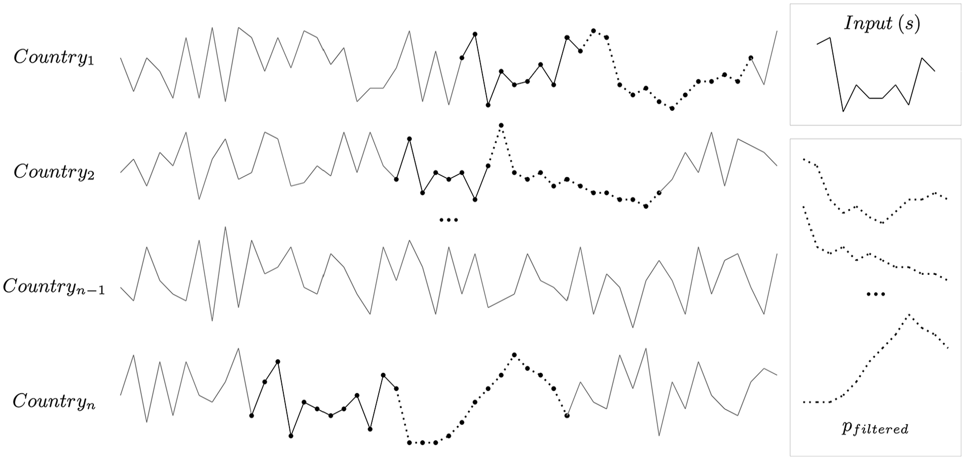
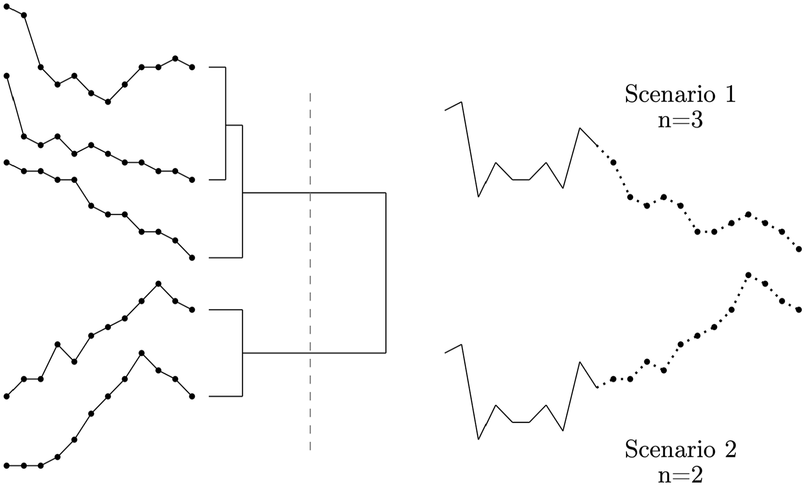
The input sequences consist of the last 10 months prior to the testing period. The reference repository $p$ contains overlapping sub-sequences of 8–12 months. For each input sequence $s$ , only the most similar sub-sequences are retained in the filtered repository $p_{f i l t e r e d} .$ Similarity is measured using Dynamic Time Warping, and a sequence is included if its distance to $s$ is below a set threshold.

Figure 3.

Agglomerative hierarchical clustering. The five sequences on the left, part of $p_{f i l t e r e d}$ , are used as input to the agglomerative hierarchical clustering. On the right, the two scenarios created by the clustering are displayed. The centroid from the majority cluster is select as the prediction. In this example, the centroid from the majority cluster is scenario 1.

Creating the reference repository

The input sequences are the last 10 months before the testing period for each country.³ The reference repository $p$ is constructed by partitioning each country’s historical data into overlapping 10-month sequences using a rolling window approach. For example, Mozambique’s sequences include January to October 1995, February to November 1995, and so on. We also consider changing the window ( $w i n$ ) to $\pm 2$ months (i.e. sub-sequences ranging from 8 to 12 months) to account for temporal variations in the speed of events.⁴ This generates a set of $N$ sequences derived exclusively from the training data. We compare each input sequence $s$ to all sequences in the reference set $p$ using Dynamic Time Warping (discussed next). Only the most similar sequences are retained, creating a filtered reference repository $p_{f i l t e r e d}$ . This ensures that only the most analogous patterns are considered for future predictions.

We use DTW to measure the similarity between our input sequence $s$ and the sequences in the reference repository $p$ . DTW is a widely used time series alignment technique that quantifies the similarity, or distance, between time series data (Keogh and Ratanamahatana, 2005). Unlike traditional methods, DTW finds the optimal alignment between two time series without being restricted to fixed temporal indices. It compares each data point in the first time series with several data points in the second, matching each to its closest counterpart. This makes it possible to stretch or compress the axis in time, which produces a new alignment between the two sequences.⁵

Using DTW as a distance metric for sequence comparison offers several advantages – most notably its invariance to time shifting and stretching. Traditional distance metrics, like the Euclidean distance, are sensitive to temporal distortions, making them less suitable for comparing time series data where temporal shifts are common (Keogh and Ratanamahatana, 2005). Consider the following three sequences: $a = [1, 2, 3, 2, 1],$ $b = [2, 3, 2, 0.5, 1]$ and $c = [1, 3, 1]$ . All three sequences have the same basic shape – first up, then down. Yet, standard approaches such as regression or the Euclidean distance are unable to find similarities between these sequences due to a strict case-by-case comparison. In contrast, DTW can align sequences that may have similar patterns but occur at different speeds or scales. Additionally, this method accommodates slight variations in sequence lengths when making comparisons, which further increases the flexibility of the approach (Wong and Wong, 2003). The DTW distance between $a$ and $b$ is 1.118 versus 2.291 for the Euclidean distance. The DTW distance between $a$ and $c$ is 1.414, while the Euclidean distance is undefined in this case due to their differing lengths. DTW is therefore ideal for matching sequences in our dataset of country-month fatalities, where temporal variations are natural occurrences.

After calculating the distance for each pair of input and historical subsequence, we filter out the sequences that do not closely match subsequence $s$ . More precisely, we keep a past subsequence $s_{u \leq t}$ in the set only if $d i s t (s, s_{u \leq t})$ is below a certain threshold ( $d i s t$ ). The threshold is initiated as $d i s t (s, s_{u \leq t}) = 0.1$ , and increases by $0.1$ until there are at least five reference subsequences in $p_{f i l t e r e d}$ . The filtered set of past subsequences is then used to make predictions. Considering only a filtered set of past sequences $p_{f i l t e r e d}$ yields riskier predictions, given that only the most similar reference series are taken into account.

The threshold $d i s t$ is a hyperparameter of the Shape finder to control the size of the filtered reference repository. A higher threshold results in a more diverse set of references, considering historical cases with a higher dissimilarity in shape. The hyperparameter is optimized by calculating out-of-sample predictions for various values of $d i s t$ in a validation period (the 12 months of 2021) and selecting the value that yields the best performance, $d i s t = 0.1$ (Figure A.1 in the Online Appendix). Our findings either do not change substantively or performance worsens when increasing the threshold $d i s t$ , which enlarges the size of the filtered repository by construction (Figure A.13 in the Online Appendix).

Predictions

For each input sequence $s$ (the last 10 months prior to the testing window), we access the sequences stored in the filtered repository of historical cases $p_{f i l t e r e d}$ . From each reference sequence, we extract the future, which is the number of fatalities for the next 12 months following that reference sequence.⁶ We then use these futures to make predictions for our input sequence $s$ . The model returns predictions for all input sequences that are not flat, meaning they have at least one month with non-zero fatalities. For flat input sequences, the model predicts zeros for the next 12 months. In those cases, predicting zero is the best guess.⁷ We use this step to speed up computation, given that flat inputs are passed on and the Shape finder algorithm is not applied in those instances.

To obtain predictions, we apply the agglomerative hierarchical clustering algorithm, using the futures of the sequences in the reference repository as input. The predicted outcome is the centroid of the cluster with the highest number of observations (the ‘majority cluster’). This clustering approach has the advantage of grouping similar futures together, which enables the identification of common patterns that might indicate recurring trends. Further, considering clusters rather than individual sequences reduces noise and discards outlier cases.

Agglomerative hierarchical clustering works by repeatedly merging observations into larger clusters based on similarity until all cases are assigned to one single group at the top (Müllner, 2011). A cut-off value ( $c u t$ ) is used to control the depth of the clustering tree, thereby specifying the final number of clusters. Selecting a lower value for $c u t$ leads to a lower cut-off value in the clustering tree and by extension a higher number of clusters. We refine the hierarchical structure by optimizing the cut-off value brute-force, which means that $c u t$ is another hyperparameter of the Shape finder algorithm.⁸ While we optimize $c u t$ using the validation data (the 12 months in 2021), increasing or decreasing the value of $c u t$ slightly does not significantly change the performance (Figure A.13 in the Online Appendix).

Based on the clustering solutions, we derive predictions for the next 12 months. We first select the cluster with the largest number of sequences – the majority cluster – and calculate the centroid, which is the average of all sequences in that cluster. That centroid is our prediction for the 12 months following the input sequence.⁹ This approach ensures that we select the most robust future – the one which is substantiated by the highest number of observations – thereby circumventing any sparsity concerns due to low numbers of cases assigned to each cluster.¹⁰

Compound model

Risk-averse and risk-taking models offer complementary strengths in conflict prediction. While risk-averse models excel at forecasting high-intensity conflicts based on recent history, they may overlook the potential escalation of medium-intensity cases (Hegre et al., 2022). In other words, risk-averse models are good at predicting a baseline risk of armed conflict accurately, while they cannot capture sudden surges and declines in fatality data. These models are risk-averse because they perform well in terms of average error, and they produce fewer overpredictions. Simultaneously, they cannot address variability and miss important short-term developments. Understanding when medium-intensity cases escalate to full-scale war is particularly important for policymakers, potentially allowing them to intervene before a more substantial escalation of violence (Mueller and Rauh, 2022).

This is the strength of a risk-taking approach – the Shape finder – which seeks to capture variability in fatality time series. However, taking risks does not always pay off, and such models are more prone to overpredictions. The effectiveness of this risk-taking approach depends on the model’s confidence in its predictions. To optimize our forecasting, we must determine when the potential benefits of risk-taking outweigh its costs. We aim to leverage the strengths of both risk-averse and risk-taking models by constructing a compound model.

The Shape finder requires sufficient observations in the historical dataset to produce accurate estimations. An insufficient data basis may lead to predictions being highly affected by outliers, making the model prone to overpredictions. Hence, we propose a compound model that includes predictions from the risk-taking Shape finder when confidence in the prediction is high. The VIEWS ensemble – a risk-averse model – is selected when confidence is low or when the severity of the input is too high, resulting in an elevated risk. An overprediction for high severity cases is likely to drive up the prediction error.

Based on these considerations, the compound employs two selection criteria – the severity of violence and the confidence level of the Shape finder. First, a risk-averse model might perform better for high intensity cases, given that any type of overprediction would lead to a high error. The severity of violence is indicated by the number of fatalities – the higher the fatalities, the higher the severity. Second, we use the clustering results as an indication of the confidence in our prediction. The confidence in the Shape finder is quantified by the relative frequency of cases assigned to the majority cluster, normalized by the logarithm of the number of matches. We select the Shape finder for cases where the observed pattern has occurred more than three times in the past and at least 50% of the historical futures of that pattern fall within the majority cluster. These two components are important for a sufficient understanding of a specific pattern and its projected outcome, and produce a compound model where 66% of the predictions are from the Shape finder, and 33% from VIEWS.¹¹

Evaluation

We compare the performance of the Shape finder to three alternatives – the VIEWS ensemble and two baselines. The first baseline – the null model – predicts zero fatalities for all country-months. The second baseline – the $t - 1$ model – uses the input sequence as prediction. These baselines may appear simplistic. However, forecasting that fatalities are zero or will remain consistent with the immediate past is a robust prediction due to the highly skewed nature of fatality data. Indeed, the null model is challenging to beat in terms of prediction error, since a large fraction of observations actually do take a value of zero. The $t - 1$ model may mirror how practitioners make predictions in the field. In the absence of any other information, someone in the field is likely to predict a continuation of the fatalities from the previous month. Ideally, we would also like to compare the Shape finder to an operational conflict prediction system. However, these are run by governments or private entities, and predictions are therefore not publicly available (see Rød et al., 2024).

The VIEWS ensemble is a more sophisticated approach and combines predictions from a variety of thematic models, using variables on among others conflict history, economic development and political institutions (Hegre et al., 2022). The VIEWS model was first introduced in 2019 and is arguably the most advanced conflict prediction model accessible to the public. The VIEWS ensemble is therefore our primary comparison for assessing the Shape finder’s performance. Our aim is not to position these models as competitors, but rather to explore how risk-averse and risk-taking approaches can complement each other, along the unique strengths of both approaches. The risk-averse model can capture a baseline risk of armed violence, and the risk-taking model is able to mirror variability in fatality time series, despite occasional over-predictions. The goal is to generate predictions that can capture variability, while maintaining a prediction error similar to existing approaches.

We report two evaluation metrics. The first is the mean squared error (MSE), a standard metric which reports the average prediction error. More formally, the MSE is defined as the average of the squared differences between predicted and observed values,

M S E = \frac{1}{n} \sum_{i = 1}^{n} {(Y_{i} - \hat{Y_{i}})}^{2}

(1)

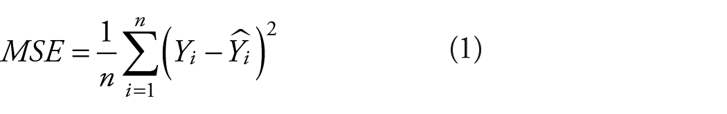
Despite its ubiquity, the MSE has severe limitations because of its propensity to reward overly conservative forecasts when the data distribution is skewed (Hossin and Sulaiman, 2015). Because conflict fatalities are heavily skewed, optimizing on the MSE can encourage risk-averse predictions. Predicting zero fatalities for all country-months yields a low MSE because most countries are at peace most of the time. This is exacerbated by the square term in the MSE, which severely punishes deviations from observed values, and therefore encourages conservative predictions. Indeed, judging by the MSE alone, there is no significant difference between the predictions of VIEWS and those of a model that only predicts zero (Figure 4).

Figure 4.

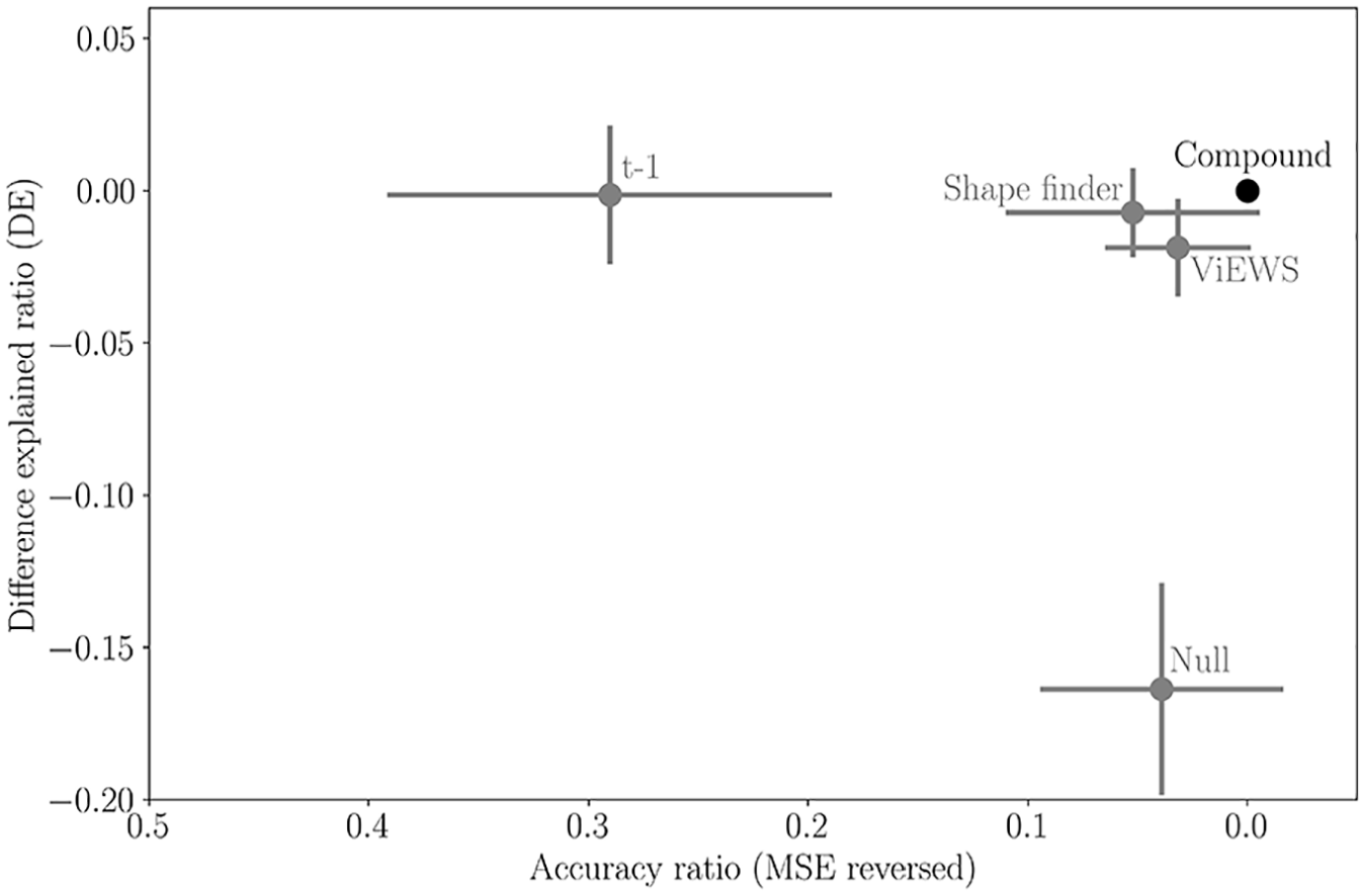
Mean log-ratio for Difference Explained (DE) and mean squared error (MSE). The log-ratios are computed using the compound as base. For DE, a negative log-ratio signifies that the compound outperforms the reference model. Conversely, for MSE, a positive log-ratio indicates that the compound performs better. For visualization purposes, we reverse the MSE axis, now showing the accuracy ratio. Superior models are located in the top-right quadrant. Vertical and horizontal bars represent the 95% confidence intervals around the mean for each metric. 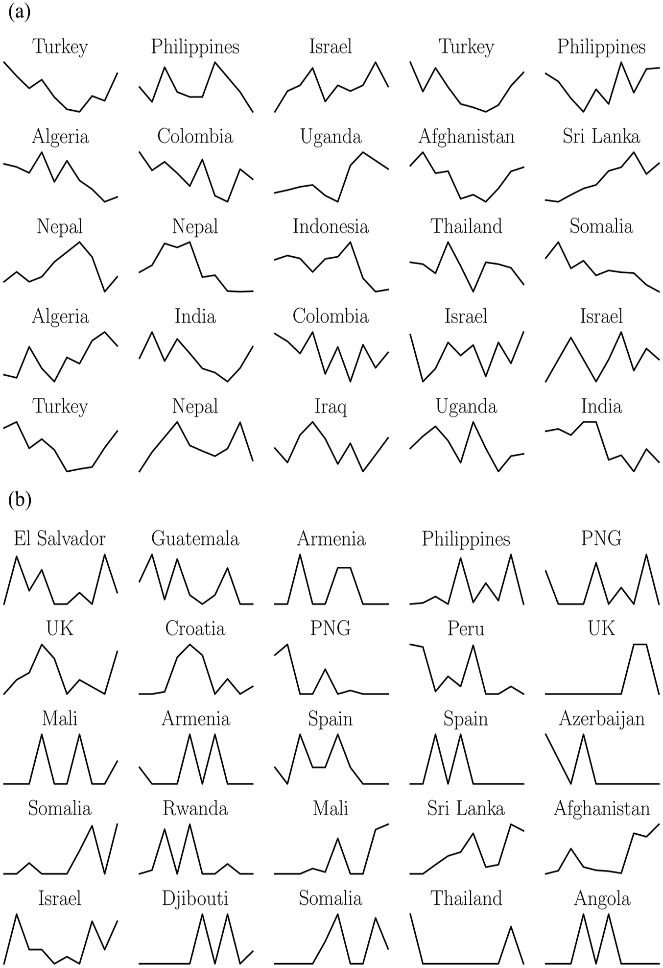We calculate the confidence intervals as $\pm 1.993 * S t a n d a r d d e v i a t i o n / \sqrt{n}$ , where 1.993 corresponds to the critical value of $t$ with 73 degrees of freedom.

The MSE does not reward predictions that capture the variability of rare events. Yet, we believe that this variation – the changes over time, rather than the repetition of the last observation – is of main interest. Indeed, relying solely on MSE might mask the model’s shortcomings in identifying variability in fatality data. Therefore, our second evaluation metric is designed to measure the algorithm’s ability to capture changes in the number of casualties, rather than capturing a stable value. To this end, our metric quantifies the degree to which our forecasts successfully detect and represent shifts, surges, or declines in casualties. We use the difference of the predicted variation, exponentially and difference weighted, to reward good predictions of peak values. This metric, which we call the Difference Explained (DE) is defined as

D E = \frac{1}{n} \sum e^{\frac{- k | Δ \hat{y} - Δ y |}{Δ y}},

(2)

where $\hat{y}$ is the predicted change, $y$ is the actual change, $n$ is the number of predictions, and $k$ is a balancing factor discussed in the next paragraph and in Note 12. $Δ$ refers to the change from $t - 1$ to $t$ (i.e. $y_{t} - y_{t - 1}$ ).

This metric offers several advantages for evaluating the accuracy of time series predictions. First, DE captures the percentage deviation between the predicted and actual changes in the time series data ( $\frac{Δ \hat{y} - Δ y}{Δ y}$ ). Second, the inclusion of an exponential term with balancing factor $e^{- k}$ introduces a nonlinear weighting that penalizes larger deviations between predicted and observed changes. Here we set $k = 5$ .¹² Larger DE values indicate a model that better captures variability.

In addition, we want to reward accurate predictions with a time shift of a single month – these are cases where a peak in fatalities is predicted either one month too early or one month too late. To allow for this time flexibility, the DE at $Δ y_{t - 1}$ and $Δ y_{t + 1}$ is obtained and a penalty of 50% is applied, meaning that the DE at $t - 1$ and $t + 1$ is multiplied by $0.5$ . The final DE value is the maximum of these three values: $t - 1$ , $t$ , or $t + 1$ . This approach rewards accurate peak predictions, even with a one-month lag. Indeed, a one-month lag can be considered a minor deviation, given the model’s 12-month prediction horizon. Overall, the DE metric is particularly useful in scenarios where the prediction of peak values is important.¹³

Results

A conflict prediction model would ideally perform well on both tasks – minimizing the prediction error and capturing meaningful variation in fatalities. The null model has a low prediction error, since most country-months experience zero fatalities – the data is highly skewed. However, such a model entirely misses variability – sudden surges or declines. The $t - 1$ model might be able to capture some variability but makes larger errors because of its simple algorithm. The VIEWS ensemble and the Shape finder address both tasks, having high accuracy and the ability to capture variability. However, VIEWS as a risk-averse model has higher accuracy, while the Shape finder as a risk-taking model has better ability to capture variability (Figure 4).

Compound model

Our main findings are summarized in Figure 4, which shows the DE and MSE for each model compared to the compound. More specifically, we calculate the log-ratio for each metric, taking the compound as base.¹⁴ For DE, a negative log-ratio signifies that the compound performs better than the reference model. For MSE, a positive log-ratio means that the compound is the better performer. The best performing models are located in the upper right quadrant, since we reversed the MSE axis now showing the accuracy ratio. All model variants – the Shape finder, the VIEWS ensemble and the two baselines – have a negative log-ratio on DE and a positive log-ratio on MSE. This means that the compound outperforms all other model variants, both in terms of having a lower prediction error and in terms of accurately capturing the variability in fatality data. The compound is able to combine the strength of VIEWS and that of the Shape finder.¹⁵

Next, we examine under which conditions the Shape finder works particularly well or poorly, in comparison to the VIEWS ensemble. We consider three characteristics of the input sequences: the standard deviation of the input sequence, the standard deviation of the differentiated input sequence and the mean of all data points in the input sequence. These three measures indicate the level of variability – a high mean value and a low standard deviation of the differentiated series suggests that the fatality sequence has substantial surges and declines. Plotting these characteristics against each other reveals clusters of cases with a positive MSE log-ratio (VIEWS as base and Shape finder as reference), suggesting that the Shape finder performs better, and clusters of cases with a negative MSE log-ratio, implying that VIEWS has a lower error.¹⁶

The Shape Finder model works particularly well for complex input shapes, which have a high average value and a small standard deviation of the differentiated series. Those two characteristics refer to sequences with substantial variability (Figure A.12 in the Online Appendix), other than flat time series, with single peaks, which would result in a high standard deviation of the differenced series and a low mean value. In these cases, VIEWS often produces either overpredictions or overly conservative forecasts. For input shapes with low complexity, having low average values and high standard deviations – typically time series with single peaks and flat trajectories (Figure A.12 in the Online Appendix) – the Shape finder tends to overpredict, while VIEWS provides more accurate forecasts.

Well-performing cases

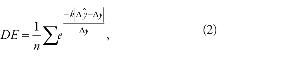
In Figure 5a, we present the cases in the well-performing cluster with the highest MSE log-ratio. For the first two inputs, we observe that the VIEWS ensemble tends to overpredict, likely due to the high mean value in the input shapes. This overprediction might explain why the Shape finder achieves higher accuracy for those cases, in addition to capturing variability.¹⁷ This contradicts the idea that risk-averse models systematically underpredict fatalities. For the last two input series, we observe that the VIEWS ensemble produces overly conservative predictions ranging around the mean, while the Shape finder is able to capture the variability. This is in line with our discussions on risk-averse and risk-taking models.

Figure 5.

Comparison of input series and predictions for best (a) and worst (b) cases. Input series are to the left of the vertical line. The solid line represents actuals, the dotted line represents VIEWS predictions, and the dashed line represents Shape finder predictions. For high complexity input series with substantial variability (a), Shape finder provides more accurate predictions and captures variability, while VIEWS either over- or underpredicts. For low complexity (b), Shape finder produces overpredictions, while VIEWS offers more accurate forecasts.

Poorly-performing cases

In Figure 5b, we present the cases in the poorly-performing cluster with the lowest MSE log-ratio. Low complexity input series lead the Shape finder to overpredict, sometimes significantly. This issue may arise because the model allows a pattern with a low cumulative sum of fatalities to be matched with a high sum case. Patterns with one or two peaks otherwise surrounded by zero fatalities typically occur in low-intensity contexts. When high-intensity cases share these patterns, they are matched with low-intensity cases, causing overpredictions.¹⁸

Characteristics of well- and poorly-performing cases

Finally, we investigate the characteristics of well- and poorly-performing input sequences. For well-performing cases, we randomly sample sequences with a high mean value and low standard deviation of the differentiated sequence (Figure 6a). For poorly-performing cases, we randomly select observations with a low mean value and a high standard deviation (Figure 6b). These are the characteristics which serve to identify clusters of well- and poorly-performing cases, when comparing the Shape finder to the VIEWS ensemble (for further details, see Figures A.9 and A.10 in the Online Appendix).

Figure 6.

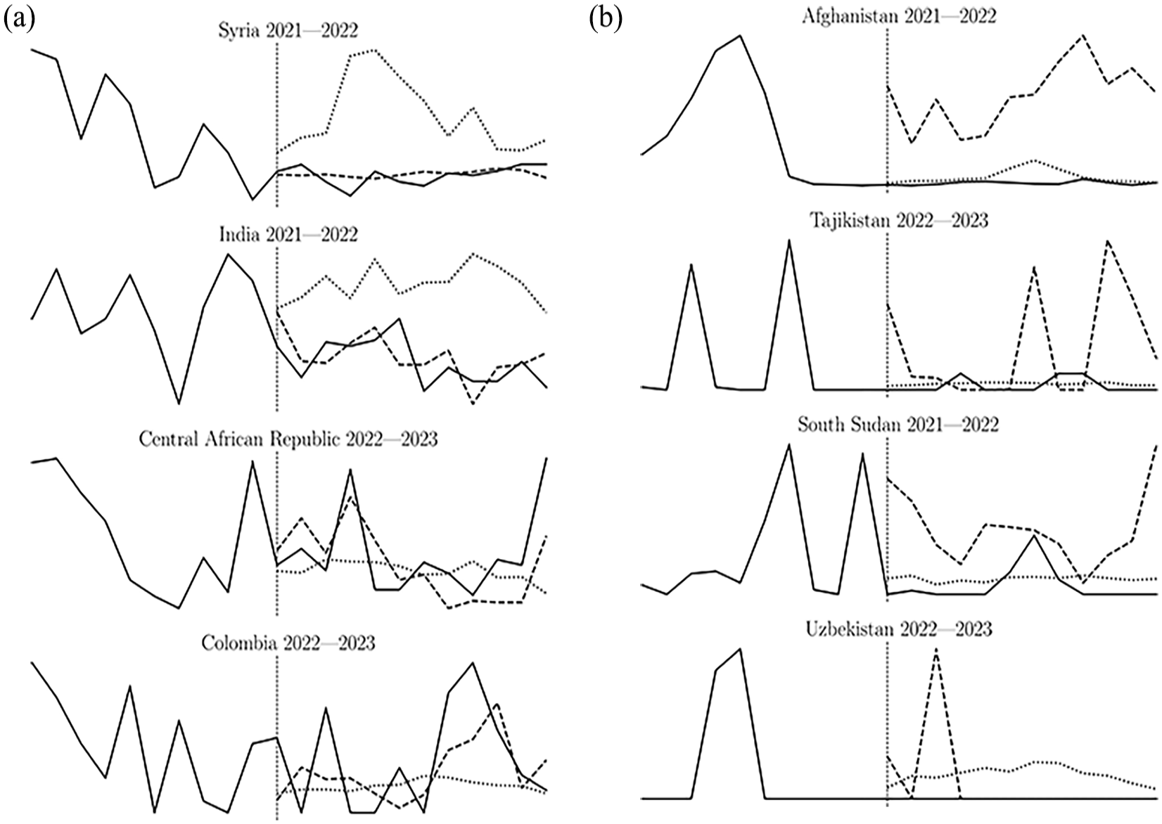
(a) Well-performing input sequences, selected because they have a high mean value and a low standard deviation of the differentiated input sequence. These are high complexity cases, presenting multiple ups and downs in the number of fatalities. The Shape finder seems particularly suitable for those types of cases. (b) Poorly-performing input sequences, selected because of a low mean value and a high standard deviation (UK = United Kingdom, PNG = Papua New Guinea). These are low complexity cases, presenting single peaks in the middle of zero fatalities. The Shape finder produces overpredictions in those cases, and VIEWS seems more suitable.

The high performing cases correspond to high complexity series, showing high variability with several ups and downs. These shapes have a high mean and a low standard deviation of the differentiated input. Combining those two characteristics reveals sequences with substantial variability, in contrast to flat time series, with single peaks, having a high standard deviation of the differenced series and a low mean. The characteristics of high complexity inputs are most pronounced in Afghanistan, India, Colombia, and the Philippines, all countries with high battle activity (Figure 6a). In other words, the Shape finder performs well when there is substantial armed violence.

For the poorly-performing clusters, we find mostly cases with low complexity, where the input sequences have a relatively low mean value and high standard deviation. These low complexity inputs are characterized by one or two peaks or a small plateau of elevated values followed by a sharp decline, or in other words, low variability. The poorly-performing cluster contains cases such as Spain, Djibouti, the United Kingdom (UK), and Papua New Guinea (PNG) presenting single peaks in fatality counts, and otherwise a value of zero.¹⁹

Robustness checks

To ensure the robustness of our findings, we conduct a series of tests in addition to tuning the Shape finder’s hyperparameters $d i s t$ and $c u t$ . The tests fall into two main categories: robustness to model specification changes and robustness to variations in model evaluation.

First, we find that changing the window length ( $w i n$ ) from ±2 (i.e. 8–12 months) to ±0, ±1 or ±3 months does not significantly affect performance (Figure A.13 in the Online Appendix). However, larger windows significantly raise computational costs, such that enlarging the window beyond what we use becomes prohibitively costly. We also explore alternative prediction approaches, including methods that do not involve forecasting based on the majority cluster. One alternative approach involves selecting the closest matches without employing clustering – for instance, directly predicting the future of the input sequence based on the future of the most similar historical pattern. We evaluate the use of the best one, three, and five matches as predictive references; however, this approach significantly underperforms compared to the Shape finder methodology (Figure A.13 in the Online Appendix). The primary issue with relying on the top matches is the increased likelihood of selecting futures based on outlier cases, which undermines the robustness and reliability of the forecasts.

As a placebo test, we also validate the performance of randomly selecting references from the repository instead of using the matched sequences. As expected, this approach leads to a notable decline in performance, particularly in terms of mean squared error (MSE), as shown in Figure A.13 in the Online Appendix. This outcome underscores the inherent challenge of simultaneously improving both the MSE and the explained variance. Another placebo test involves generating predictions using clusters other than the largest ones. As expected from our premise that larger clusters represent more consistent and reliable patterns, predictions based on smaller or non-dominant (e.g. median) clusters result in less accurate forecasts, which reinforces the importance of focusing on the majority cluster for robust predictions (Figure A.14 in the Online Appendix). This finding aligns with the expectation that when past sequences consistently converge on a particular outcome, that outcome serves as the most reliable predictor for similar patterns.

We also verify that the predictions are well calibrated, meaning that when 90% of matches are assigned to the majority cluster, 90% of the futures of the cases in the cluster would also be assigned to the majority cluster. This would further support the conclusion that the clusters contain meaningful and predictive information. While calibration is not perfect (Figure A.15 in the Online Appendix), we do observe that the larger the relative size of the majority cluster, the more futures get assigned to that cluster as well. Finally, we also confirm that our main findings do not change significantly when increasing or decreasing the balancing factor $k$ in the DE formula (Figure A.5 in the Online Appendix). And we demonstrate that using the DTW distance between predicted and actual futures as a metric instead of DE does not change our findings either (Figure A.7 in the Online Appendix).

Discussion

The Shape finder offers several advantages in comparison to existing conflict prediction models. First, identifying similar historical cases enhances interpretability, enabling researchers to understand how specific predictions are generated – a key characteristic of a trustworthy model (Masís, 2023). Related to this, the inner-workings of the Shape finder are transparent and can easily be comprehended by humans, which is an advantage over similar approaches using deep learning (e.g. Liao et al., 2022; Vafa et al., 2024). This is particularly important in conflict prediction, where practitioners are likely concerned about the trustworthiness of black-box predictions. Second, the Shape finder is entirely autoregressive, requiring no covariates unlike VIEWS and other prediction models. This is particularly advantageous given that most social science data are rarely available at a disaggregated level, making them difficult to use in machine learning applications for complex phenomena such as armed conflict.

Our approach of adjusting the reference repository leads to substantial improvements compared to previous methods that consider all historical cases without filtering (Chadefaux, 2022). By including only the most analogous cases in the reference repository, the Shape finder produces more dynamic and accurate forecasts. While the Shape finder has limitations, such as the inability to predict fatalities following a flat period, so-called onset cases, its biggest advantage remains its simple autoregressive set-up. Requiring only fatality data and no other correlates, the simple Shape finder achieves performance comparable to much more complex models, such as VIEWS (Figure 4). The VIEWS ensemble combines several constituent models, with at times hundreds of variables (Hegre et al., 2022). This architecture likely requires substantial computational resources. In contrast, predicting 12 months for all countries takes the Shape finder less than 2 hours on a regular desktop computer.

Anticipating conflict onsets – the ‘hard problem of conflict prediction’ (Mueller and Rauh, 2022: 2442) – is another area where current conflict prediction models fall short. Based on the autoregressive set-up of the Shape finder, our model cannot forecast conflict onsets either, in other words, the model returns flat predictions based on flat input sequences. Countering this shortcoming, one possible alternative could be a compound model, combining an onset model with the Shape finder. Incorporating variables with more variation, such as news topics (Mueller and Rauh, 2018) or protest indicators, might help address the challenge of predicting conflict onsets.

Conclusion

Conflict prediction has evolved as a thriving subfield of peace research due to its practical relevance (Hegre et al., 2017) and potential for theory validation (Colaresi and Mahmood, 2017). However, forecasting fatalities in armed conflict remains a challenging prediction task. The right skewness of fatalities often leads to overly conservative predictions close to the mean, resulting in risk-averse models which struggle to account for sudden surges and declines in violence. While these models produce accurate predictions when judged by the mean squared error, they fall short in capturing the variability crucial for practitioners seeking to intervene before substantial escalations of violence (Mueller and Rauh, 2022).

This article introduces the ‘Shape finder’, a risk-taking approach designed to complement existing risk-averse methods in conflict prediction. The Shape finder’s primary advantage lies in its ability to explain variability in fatalities, including sudden escalations or de-escalations. By finding recurring patterns in time series of fatalities and filtering the most similar historical cases into a reference repository, the Shape finder produces more dynamic forecasts. This approach is based on the assumption that similar patterns in the past lead to similar patterns in the future. Patterns in fatality data represent observable implications of interactions between governments and non-state armed groups.

To leverage the unique advantages of both risk-averse and risk-taking approaches, we constructed a compound model combining the Shape finder and the VIEWS ensemble (Hegre et al., 2022) – the most sophisticated prediction model in the field. The compound model is constructed based on the confidence in the Shape finder predictions and the severity of violence, and performs significantly better than both constituent models and two technical baselines: the null model and the $t - 1$ model. Notably, the Shape finder excels in high complexity cases with multiple fluctuations, where VIEWS tends to produce overpredictions or overly conservative forecasts. Conversely, VIEWS performs better in low complexity cases, where the Shape finder tends to overpredict. In simple words, the Shape finder is particularly suitable when there is substantial armed conflict.

In conclusion, the Shape finder offers a valuable complement to existing risk-averse approaches in conflict prediction. Its ability to capture variability in fatalities, coupled with its interpretability and autoregressive nature, makes it a promising tool for researchers and practitioners in the field of peace research and conflict studies. The Shape finder is likely to be helpful in the study of social phenomena with a similar data structure than armed conflict – in particular, rare events, such as protest, riots, and violence against civilians. The theoretical arguments put forward here likely apply to other forms of armed violence and political contention more generally – the interactions between the state and an opposition group produce recurring patterns in sequences of events, which are indicative of the future.

Footnotes

Acknowledgements

We would like to thank all participants at the VIEWS Prediction Competition Workshop 2023, in particular Håvard Hegre, Paola Vesco, the German Federal Foreign Office (FFO), and PREVIEW (Prediction, Visualisation, Early Warning), as well as the reviewers and editors at Journal of Peace Research for constructive feedback and helpful comments.

Replication data

The dataset and do-files for the empirical analysis in this article, along with the Online Appendix, are available at https://www.prio.org/jpr/datasets/ and . All analyses were conducted using Python 3.8.5.

Funding

The authors disclosed receipt of the following financial support for the research, authorship, and/or publication of this article: This project has received funding from the European Research Council (ERC) under the European Union’s Horizon 2020 research and innovation programme (grant agreement No 101002240), and the Irish Research Council (IRC) in partnership with the Department of Foreign Affairs (DFA) under the Andrew Grene Postgraduate Scholarship in Conflict Resolution (Grant number GOIPG/2023/3883).

ORCID iDs

Thomas Schincariol

Hannah Frank

Notes

THOMAS SCHINCARIOL, b. 1997, MSc in Control and Computer Engineering (University of Technology of Troyes, 2021); PhD Candidate, Department of Political Science, Trinity College Dublin (2021–present).

HANNAH FRANK, b. 1994, MSSc in Peace and Conflict Studies (Uppsala University, 2021); PhD Candidate, Department of Political Science, Trinity College Dublin (2021–present).

THOMAS CHADEFAUX, b. 1980, PhD in Political Science (University of Michigan, 2009); Professor, Department of Political Science, Trinity College Dublin (2021–present).

References

ACLED (2023) ACLED CAST methodology. Armed Conflict Location and Event Data (ACLED). Available at: https://acleddata.com/acleddatanew/wp-content/uploads/dlm_uploads/2023/07/ACLED-CAST-Methodology-%E2%80%93-July-2023.pdf (accessed 11 February 2025).

Axelrod

(1990) The Evolution of Cooperation. London, New York: Penguin Books.

Beardsley

Cunningham

White

(2019) Mediation, peacekeeping, and the severity of civil war. Journal of Conflict Resolution 63(7): 1682–1709.

Cederman

Weidmann

(2017) Predicting armed conflict: Time to adjust our expectations? Science 355(6324): 474–476.

Chadefaux

(2017) Conflict forecasting and its limits. Data Science 1(1–2): 7–17.

Chadefaux

(2022) A shape-based approach to conflict forecasting. International Interactions 48(4): 633–648.

Colaresi

Mahmood

(2017) Do the robot: Lessons from machine learning to improve conflict forecasting. Journal of Peace Research 54(2): 193–214.

Davenport

(2007) State repression and political order. Annual Review of Political Science 10: 1–23.

Della Porta

(2008) Research on social movements and political violence. Qualitative Sociology 31(3): 221–230.

10.

Della Porta

Hall

Poljarevic

, et al. (2018) Social Movements and Civil War: When Protests for Democratization Fail. Abingdon: Routledge.

11.

Diz-Pita

Otero-Espinar

(2021) Predator–prey models: A review of some recent advances. Mathematics 9(15): 1783.

12.

Dosi

Usula

Virgillito

(2024) Increasing returns and labor markets in a predator–prey model. Journal of Evolutionary Economics 34: 375–402.

13.

Gleditsch

Ward

(1999) A revised list of independent states since the Congress of Vienna. International Interactions 25(4): 393–413.

14.

Gleditsch

Wallensteen

Eriksson

, et al. (2002) Armed conflict 1946–2001: A new dataset. Journal of Peace Research 39(5): 615–637.

15.

Hegre

Akbari

Croicu

, et al. (2022) Forecasting fatalities. Violence Early-Warning System (ViEWS). Available at: http://uu.diva-portal.org/smash/get/diva2:1667048/FULLTEXT01.pdf (accessed 11 February 2025).

16.

Hegre

Allansson

Basedau

, et al. (2019) ViEWS: A political violence early-warning system. Journal of Peace Research 56(2): 155–174.

17.

Hegre

Bell

Colaresi

, et al. (2021) ViEWS 2020: Revising and evaluating the ViEWS political violence early-warning system. Journal of Peace Research 58(3): 599–611.

18.

Hegre

Metternich

Nygård

, et al. (2017) Introduction: Forecasting in peace research. Journal of Peace Research 54(2): 113–124.

19.

Hethcote

(1989) Three basic epidemiological models. In: Levin

Hallam

Gross

(eds) Applied Mathematical Ecology. Berlin and Heidelberg: Springer, 119–144.

20.

Hossin

Sulaiman

(2015) A review on evaluation metrics for data classification evaluations. International Journal of Data Mining & Knowledge Management Process 5(2): 1–11.

21.

Kalecki

(1937) A theory of the business cycle. The Review of Economic Studies 4(2): 77–97.

22.

Keogh

Ratanamahatana

(2005) Exact indexing of dynamic time warping. Knowledge and Information Systems 7(3): 358–386.

23.

King

Zeng

(2001) Explaining rare events in international relations. International Organization 55(3): 693–715.

24.

Kirk

(1996) Demographic transition theory. Population Studies 50(3): 361–387.

25.

Koopmans

(2007) Protest in time and space: The evolution of waves of contention. In: Snow

Soule

Hanspeter

(eds) The Blackwell Companion to Social Movements. Oxford: Blackwell Publishing, 19–46.

26.

Lacina

(2006) Explaining the severity of civil wars. Journal of Conflict Resolution 50(2): 276–289.

27.

Liao

Bolano

Brzinsky-Fay

, et al. (2022) Sequence analysis: Its past, present, and future. Social Science Research 107: 102772.

28.

McAdam

(1983) Tactical innovation and the pace of insurgency. American Sociological Review 48(6): 735–754.

29.

Malone

(2021) The timing of militant violence onset. Working Paper. Available at: https://www.dropbox.com/scl/fi/18r4711je60ymrp6y52a9/TimingViolenceOnset.pdf?rlkey=tgsx7urbgokl5i1z9cz4mlm85&e=1&dl=0 (accessed 11 February 2025).

30.

Masís

(2023) Interpretable Machine Learning with Python: Build Explainable, Fair, and Robust High-Performance Models with Hands-On, Real-World Examples. Birmingham: Packt.

31.

Mueller

Rauh

(2018) Reading between the lines: Prediction of political violence using newspaper text. American Political Science Review 112(2): 358–375.

32.

Mueller

Rauh

(2022) The hard problem of prediction for conflict prevention. Journal of the European Economic Association 20(6): 2440–2467.

33.

Mueller

Rauh

Seimon

, et al. (2024) The urgency of conflict prevention – A macroeconomic perspective. International Monetary Fund (IMF) Working Papers. Working Paper. Available at: https://www.imf.org/en/Publications/WP/Issues/2024/12/17/The-Urgency-of-Conflict-Prevention-A-Macroeconomic-Perspective-559143 (accessed 18 February 2025).

34.

Müllner

(2011) Modern hierarchical, agglomerative clustering algorithms. Working Paper. Available at: https://arxiv.org/abs/1109.2378 (accessed 11 February 2025).

35.

Pierskalla

(2010) Protest, deterrence, and escalation: The strategic calculus of government repression. Journal of Conflict Resolution 54(1): 117–145.

36.

Powell

(2004) The inefficient use of power: Costly conflict with complete information. American Political Science Review 98(2): 231–241.

37.

Regan

(2002) Third-party interventions and the duration of intrastate conflicts. The Journal of Conflict Resolution 46(1): 55–73.

38.

Rød

Gåsste

Hegre

(2024) A review and comparison of conflict early warning systems. International Journal of Forecasting 40(1): 96–112.

39.

Rød

Weidmann

(2023) From bad to worse? How protest can foster armed conflict in autocracies. Political Geography 103: 102891.

40.

Slantchev

(2003) The power to hurt: Costly conflict with completely informed states. American Political Science Review 97(1): 123–133.

41.

Sundberg

Melander

(2013) Introducing the UCDP georeferenced event dataset. Journal of Peace Research 50(4): 523–532.

42.

Tarrow

(2011) Power in Movement: Social Movements and Contentious Politics. Cambridge and New York: Cambridge University Press.

43.

Vafa

Palikot

, et al. (2024) CAREER: A foundation model for labor sequence data. Working Paper. Available at: https://arxiv.org/abs/2202.08370 (accessed 11 February 2025).

44.

Ward

Greenhill

Bakke

(2010) The perils of policy by p-value: Predicting civil conflicts. Journal of Peace Research 47(4): 363–375.

45.

Wong

(2003) Efficient subsequence matching for sequences databases under time warping. In: Seventh international database engineering and applications symposium, 2003. proceedings, Hong Kong, China.

46.

Young

(2013) Repression, dissent, and the onset of civil war. Political Research Quarterly 66(3): 516–532.

Accounting for variability in conflict dynamics: A pattern-based predictive model

Abstract

Keywords

Conflict prediction

Patterns in fatality data

Data

Methods

Creating the reference repository

Predictions

Compound model

Evaluation

Results

Compound model

Well-performing cases

Poorly-performing cases

Characteristics of well- and poorly-performing cases

Robustness checks

Discussion

Conclusion

Footnotes

Acknowledgements

Replication data

Funding

ORCID iDs

Notes

References