Sage Journals: Discover world-class research

Abstract

Calculating the consequences of global public bads such as climate change or pandemics helps uncover the scale, distribution and structure of their economic burdens. As violent conflict affects billions of people worldwide, whether directly or indirectly, this article sets out to estimate its global macro-economic repercussions. Using a novel methodology that accounts for multiple dimensions of war, the article finds that, in the absence of violent conflict since 1970, the level of global GDP in 2014 would have been, on average, 12% higher. When disaggregating these results by conflict type, civil conflicts are estimated to have been the costliest by far. Income growth is found to be altered up to four years following the end of a conflict, although the direction of this relationship depends on the intensity and type of conflict. Countries also suffer significantly from fighting in neighbouring countries, thereby showing the importance of mitigating spillovers rapidly. The largest absolute losses associated with violence emanate from Asia, while many high-income economies are found to benefit economically from participating in conflicts on foreign soil. This analysis thus shows that, despite some evidence of a faster post-conflict growth and possible benefits for external participants, violent conflict leads to net global losses that linger long after peace is achieved, reducing the peace dividend. The article concludes by discussing public policy options to strengthen the benefits of peace as a global public good.

Keywords

conflict spillover costs of conflict growth internal armed conflict international war peace dividend

Introduction

Public bads cost society: HIV/AIDS (Veenstra & Whiteside, 2005), malaria (Sachs & Malaney, 2002), alcoholism (Rehm et al., 2009) and diabetes (Yach, Stuckler & Brownell, 2006) reduce economic growth, as do air pollution (Larsen, 2014), climate change (Stern, 2007; Hsiang & Jina, 2014; Kalkuhl & Wenz, 2020), soil degradation (Pimentel et al., 1995), financial crises (Cerra & Saxena, 2008; Inklaar, de Guevara & Maudos, 2012) and, recently, COVID-19 (Fernandes, 2020; McKibbin & Fernando, 2020).

Likewise, violent conflict burdens society both economically and socially (Collier, 1999; Verwimp, Justino & Brück, 2009, 2019; Mueller, 2013; Serneels & Verpoorten, 2015; Bove, Elia & Smith, 2017; Costalli, Moretti & Pischedda, 2017), though the aggregate, global scale of this burden remains unclear (IEP, 2016; OCHA, 2017).

Past studies have shown that a country’s economic growth can be influenced by conflicts occurring both on its own territory (Polacheck & Sevastianova, 2012) and on its neighbours’ (Murdoch & Sandler, 2002a,b, 2004; de Groot, 2010; Dunne & Tian, 2014), and this influence can be prolonged long after the conflict is ended (Organski & Kugler, 1977; Collier, 1999; Kang & Meernik, 2005). The direction, period and factors determining these relationships are, however, still debated. Furthermore, little is known about the differential consequences for the various types of conflict participants.

We thus set out to fill this knowledge gap. Using a panel of 190 countries from 1970 to 2014, we estimate the average consequence of various dimensions of conflicts on yearly GDP growth. First, we categorize all the major conflicts¹ that took place during the observed period into three types: civil (between a state and a non-state actor), interstate (between two states) and non-territorial (participation in a civil or interstate conflict taking place entirely on foreign territory). Second, we analyse the number of years following the end of each type of conflict, during which a significant relationship continues to be observed with growth. Third, we introduce a spillover variable that measures the possible influence of each type of conflict taking place up to 1,000 km away from a country’s border. Finally, as we posit that the economic consequence of each of these conflict dimensions depends on the intensity of the episode, we use an index that quantifies conflict intensity on a scale from 0 to 10, based on a variety of factors.

Using a country-fixed effects estimation and cross-checking the robustness of the results with other specifications, we find that an additional unit of civil or international conflict intensity reduces the ‘host’ country’s yearly GDP growth by an average of 0.9% during the conflict years. On the other hand, we find a U-shaped relationship between conflict intensity and GDP growth for external participants. Secondly, civil conflicts are found to have a U-shaped influence on growth up to four years following the end of a conflict, while international conflicts seem to have a positive influence up to two years later. This thus provides some evidence for Organski & Kugler’s (1977) ‘phoenix’ effect, whereby post-conflict nations grow faster than their peaceful counterparts. Finally, spillovers from civil and international conflicts are found to be strongly detrimental to growth, while having a neighbour participating externally in a conflict is found to be economically beneficial.

As a second step, we provide a methodology to estimate what the yearly growth rate would have been in the absence of conflict. We then use this estimated rate to provide a year-by-year counterfactual GDP level for each country. We consequently find that, had there been no conflict throughout the world since 1970, global GDP would have been 12% larger in 2014.

Disaggregating our main results, we find that Asia has suffered the most from conflict; while many developed economies in North America, Europe and Oceania are found to have benefited from their participation. A potential explanation for this is that external state actors intervene in armed conflicts primarily out of their own economic and national security interests (Aydin, 2012; Bove, Gleditsch & Sekeris, 2016; Bove, Deiana & Nisticò, 2018).

Our inquiry into the global economic burden of violent conflict is structured as follows. First, we illustrate the conceptual framework used for the analysis. Next, we identify the datasets and methodology used for our empirical estimation. We then present our results, discuss their robustness and compare them with previous findings before concluding.

Conceptual framework

Although there is a clear consensus that ‘hosting’ a conflict is damaging to growth in the short term (see e.g. Bozzoli, Brück & Sottsas, 2010 for a comprehensive survey on the topic), the growth reactions to being near a conflict, participating externally and ending conflict remain unclear. We thus analyse the global dynamics surrounding conflicts to estimate their net global consequences over 45 years of observation. While this is an empirical exercise, we first consider what can be learned from the theoretical literature to help construct our empirical model.

As the literature is mostly conclusive regarding conflicts occurring within a country’s own territory, we focus on this case to graphically illustrate our theoretical framework. We discuss details of the concepts introduced here below and alternative scenarios in the following subsections.

Figure 1.

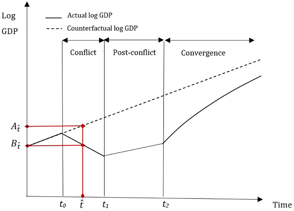
Theoretical burden of conflict

As shown in Figure 1, when a conflict breaks out in a country (at t ₀), yearly GDP growth is expected to decline. Hence, the observed GDP level goes below the GDP that the country could have experienced had there been no conflict (the ‘counterfactual GDP’). Once peace is achieved (at t ₁), the immediate post-conflict period starts. This is an adjustment period during which the past conflict continues to directly influence growth, although the direction of this influence and actual length of this period are still debated. For simplicity, the figure only shows the situation where a country’s growth rate is still reduced. From t ₂, the previous conflict no longer has an effect, except through the theory of conditional convergence (Barro & Sala-i-Martin, 1992), according to which countries with a lower GDP, ceteris paribus, will grow faster than their richer counterparts. During the entire period, the difference between counterfactual and actual GDP is the total GDP loss resulting from conflict.

As question marks still prevail on the direction, intensity and timing that define the GDP path during each of the above-mentioned subperiods surrounding conflict, we estimate average predictions for each conflict type. We next introduce the model that is the backbone for this analysis.

Empirical model

Conflict can affect GDP not only through population changes, but also by influencing other fundamental growth predictors like investment (Abadie & Gardeazabal, 2003; Chen, Loayza & Reynal-Querol, 2008) and education (Lai & Thyne, 2007; Brück, Di Maio & Miaari, 2018). In an attempt to estimate the more direct growth alterations that can emanate from conflict, we control for the three above-mentioned variables which are included in Mankiw, Romer & Weil’s (MRW) (1992) interpretation of the Solow (1956) model. With some abuse of terminology, we hereinafter refer to them as the ‘Solow covariates’.

Our empirical model takes the following form:

g r_{i, t} = β_{i} + β_{1} ln (g d p_{i, t - 1}) + β_{2} ln (i n v e s t_{i, t}) + β_{3} ln (e d u_{i, t}) + β_{4} (n_{i, t} + g + δ) + \sum β_{k} (C_{i, t, k}) + ε_{i, t}

where gr_i,t is the growth rate of country i at year t and $g d p_{i, t - 1}$ is the previous year’s aggregate GDP level, which is included to capture the average rate of convergence β₁ . $i n v e s t_{i, t}$ is the fraction of income invested in physical capital, investment in human capital is approximated through educational attainment $(e d u_{i, t})$ , $n_{i, t}$ represents labour growth, g is labour efficiency and $δ$ is the depreciation rate.² β_k is the coefficient of interest associated with conflict dimension C_k . β_i are the country-specific intercepts of the fixed effects model, and $ε_{i, t}$ includes all other time-varying unobservable shocks to GDP growth.

Possible influences of conflict on economic growth

While the use of aggregate data makes it hard to explore the mechanisms through which a conflict shapes economic performance, we build on the literature to discuss some of the processes through which conflicts influence the GDP growth of host nations, neighbours and external participants.

Current conflicts

Conflicts can have an immediate negative effect on output when they disrupt production (Blomberg, Hess & Orphanides, 2004). If public goods are destroyed, this reduces the efficiency of public expenditure. Moreover, the increased military expenditure occurring during conflict is likely to crowd out public expenditure in other areas (Knight, Loayza & Villanueva, 1996; Collier et al., 2003), including the police force. Reduced expenditure on the latter impedes the rule of law and thus the security of property rights. In response to this, private agents are likely to engage in portfolio substitutions (Weinstein & Imai, 2000) by shifting their assets out of the country (Collier, 1999), thereby potentially benefiting other nations. On top of this, if the military expenditure is financed by an increase in taxes, this could lower private consumption or create dissaving if this income reduction is seen as temporary (Collier, 1999). The longer and more intense the conflict, the larger these effects are expected to be (Costalli, Moretti & Pischedda, 2017).

Proposition 1: Civil and international conflicts negatively affect economic growth, and the effects grow with intensity.

While host countries mainly suffer from civil and international conflicts, third parties may benefit from them. External state actors tend to intervene in armed conflict primarily out of their own economic and national security interests (Aydin, 2012; World Bank, 2020). Potential benefits for third parties include enhanced access to natural resources and trade, improved national security, and geostrategic advantages (Chang, Potter & Sanders, 2007; Bove, Gleditsch & Sekeris, 2016; Bove, Deiana & Nisticò, 2018). However, intervening in a conflict on foreign soil can also exacerbate costs for the home nation if it leads to an increase in the world price of commodities produced by the host nation. One example is the price of oil in the USA, which jumped from $25 a barrel in 2007 to $140 a barrel in 2008, following their intervention in Iraq (House of Representatives Hearing, 2010: 7; Stiglitz & Bilmes, 2008).

Proposition 2: Getting militarily involved in conflicts taking place on foreign soil affects home country growth, although the sign of this correlation is a priori ambiguous.

Neighbouring conflicts

Conflicts can also affect neighbouring nations’ economic growth through their impact on labour and human capital notably. First, an increasing share of labour is likely to be assigned to unproductive activities like border protection (de Groot, 2010). Second, past findings have shown that refugees that stop at their nearest neighbours tend to be unskilled and poor (de Groot, 2010) and can carry contagious diseases (Montalvo & Reynal-Querol, 2007). Meanwhile, those who pass through their primary neighbouring countries on to secondary ones are likely to carry more human capital (Dunne & Tian, 2014), although a positive effect will hardly be observed within the short term. Finally, the presence of refugees and displaced populations can increase the risk of conflict diffusion through the transnational spread of arms, combatants and ideologies (Salehyan & Gleditsch, 2006; Choi & Salehyan, 2013).

Another burden of conflict can be found through the globalization channel. In a host country, road destruction and declining commodity production (Hendrix & Glaser, 2011) mean that domestic and international trade are hindered (Blomberg & Hess, 2006). Neighbouring states may also be negatively affected if trading routes pass through the conflicted areas or if foreign investors judge the whole region risky. On the other hand, a positive effect could be seen if neighbours become substitute trade partners (Cali et al., 2015). Furthermore, neighbours of conflict participants may increase their exports of military goods, potentially leading to a Keynesian stimulus (Keynes, 1920) for their economy.

Proposition 3: Civil, international and non-territorial conflicts influence neighbouring nations’ economic growth.

Past conflicts

Looking at post-conflict economies, reduced productivity can remain due to permanent injuries or disease spread, which require continued public health expenditure (Edwards, 2013; Dunne & Tian, 2017). Extra deaths and injuries can also take place if landmines remain (Unruh, Heynen & Hossler, 2003), and nations may suffer from continued environmental consequences including water, sanitation and biodiversity challenges (Hoeffler, 2012). Postwar agricultural production may also be dampened due to war legacies (Bozzoli & Brück, 2009). However, the direction of the post-conflict effect on economic growth is likely to depend on the gravity of the conflict. Collier (1999) found that following a one-year conflict, the five post-conflict years will have a growth rate of 2.1% below the growth path in absence of conflict. But after a 15-year conflict, this post-conflict growth is 5.9% higher than the counterfactual. Thus, countries that faced severe conflicts seem to experience a phoenix effect faster, by bouncing back to their long-term trend. This can be due to a higher amount of international support following a more intense, and possibly more mediatized, conflict, which could accelerate the reconstruction process (Miguel & Roland, 2011). Furthermore, when conflict leads to institutional reform (Slater, 2010), this facilitates the removal of exploitative governments, thereby reducing vested interests that inhibit innovation (Olson, 1982) and allowing the mobilization of resources, in turn leading to faster growth (Cramer, 2007).

On the other hand, governments that finance conflicts through expansionary monetary policy suffer its inflationary effects shortly after. Moreover, if the conflict is debt-financed, the economy will have to add interest payments to future public expenditures, thereby hampering future consumption and thus mid-term growth (Knight, Loayza & Villanueva, 1996; Smith, 2014). On top of this, economic stagnation can take place in the initial post-conflict phase because of a labour surplus

Table I.

Descriptive statistics: whole sample

Variable	Source	Average	St. dev.	Min.	Max.
Conflict variables
Probability (civil conflict), %	Major Episodes of Political Violence Project	15.91
Average civil conflict intensity (cases where civil conf. intensity > 0)	Major Episodes of Political Violence Project	3.30	1.66	1	8
Probability (international conflict), %	Major Episodes of Political Violence Project	3.02
Average intl. conflict intensity (cases where intl. conf. intensity > 0)	Major Episodes of Political Violence Project	2.83	1.81	1	7
Probability (non-territorial conflict), %	Major Episodes of Political Violence Project	10.64
Average non-territorial conflict intensity (cases where non-territorial conflict intensity > 0)	Major Episodes of Political Violence Project	3.48	1.59	1	6
GDP variables
GDP (billions of 2010 USD)	World Bank Indicators 2017 and Penn World Table v.9.0	249	985	0.07	16,200
Average GDP per capita (2010 USD)	World Bank Indicators 2017 and Penn World Table v.9.0	11,480.95	19,000.6	114.33	185,884
Average annual GDP per capita growth, %	World Bank Indicators 2017 and Penn World Table v.9.0	2.00	6.98	–66.04	141.64
Other control variables
Average investment/GDP (%)	Penn World Table v.9.0	21.40	12.44	0.56	412.11
Population (thousands)	Penn World Table v.9.0	28,900	112,000	12	1,400,000
Average education (% 20 to 24-year-old male population with some secondary schooling)	Hegre et al. (2013)	60.98	28.16	1.78	100
Burden of conflict
Average burden of conflict (billions of 2010 USD)	Own calculations	21.60	147.07	–1,909.31	3,283.80
Average economic burden of conflict indicator – EBCI (% GDP)	Own calculations, World Bank Indicators 2017 and Penn World Table v.9.0	13.93	26.05	–20.92	287.13
N	7,325

from military demobilization (Bove, Elia & Smith, 2017), or if the conflict impoverished the nation so much that it struggles to start saving or investing again (Miguel & Roland, 2011).

Proposition 4: Civil and international conflicts influence post-conflict economic growth, although the direction depends on the gravity of the conflict.

Data and methods

Data sources and variables

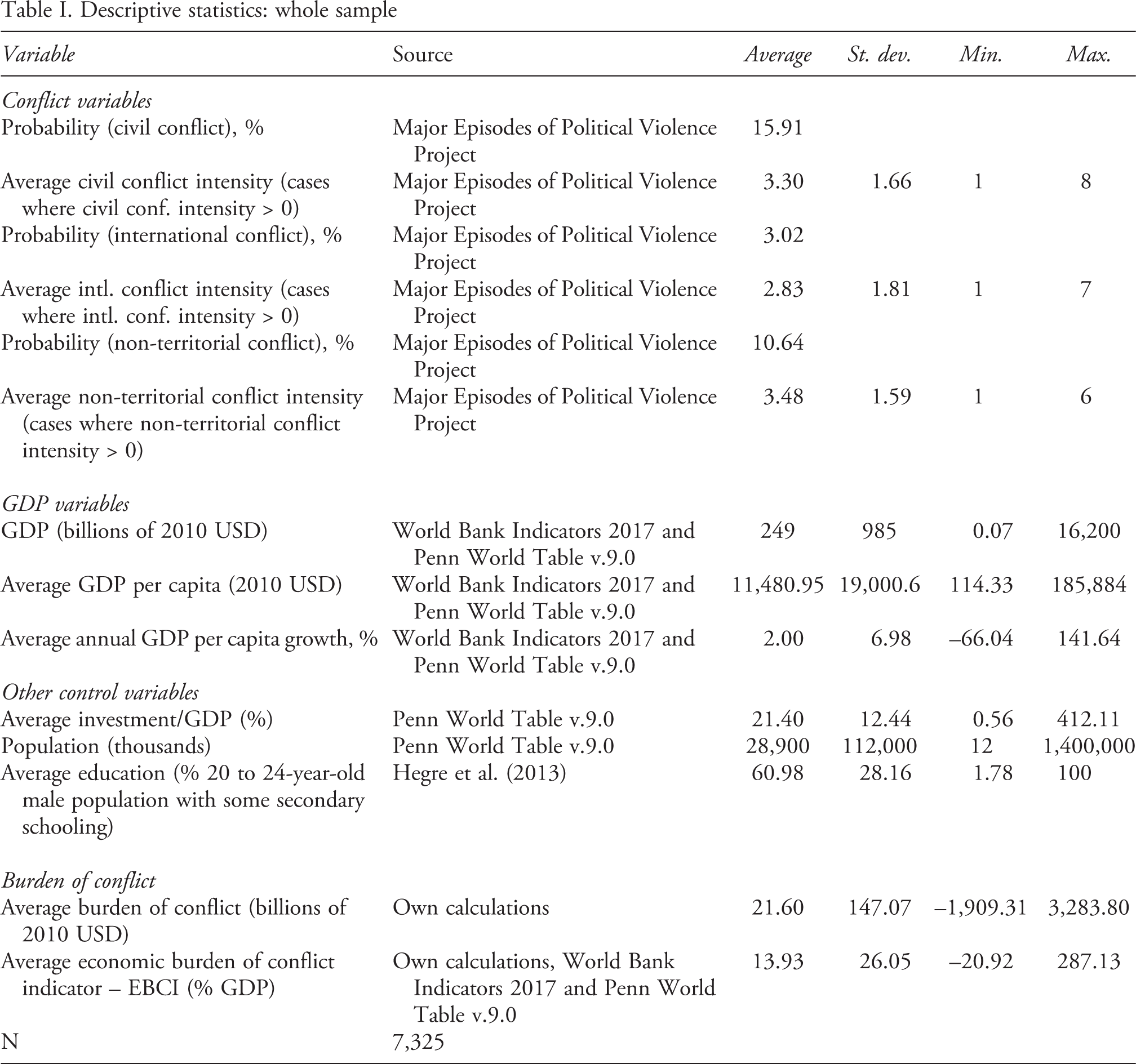
To shed light on the above-mentioned propositions, we construct an annual panel that comprises 190 countries from 1970 to 2014. We next describe our sources and variable selection process. Descriptive statistics for all variables are provided in Table I.

Dependent variable

Our main source for GDP data (in 2010 US dollars) is the World Development Indicators (World Bank, 2017). We add data from the Penn World Tables version 9.0 (PWT; Feenstra, Inklaar & Timmer, 2015) for 18 countries that are not included in the former.³ We use aggregate GDP growth as the outcome variable to capture the possibility of a decrease in output due to a decrease in population. However, we show in

Figure 2.

Conflict years per region during 1970–2014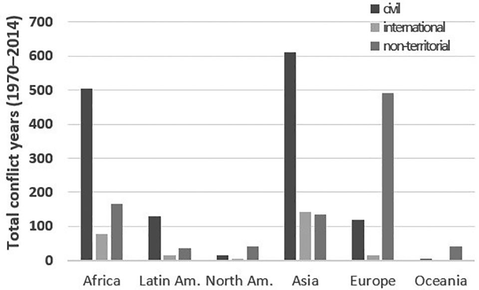

the robustness section that using per capita GDP does not alter the main results.

Current conflicts

We consider three types of conflicts: civil, interstate and non-territorial. For each type, we use Marshall & Cole’s (2014) intensity measure which uses a scale from 0 to 10. These magnitudes reflect multiple factors including state capabilities, number of deaths, capital destruction, population displacement and episode duration. Sporadic acts of terrorism are included within that scale, at magnitude 2. In order to create our non-territorial conflict variable, we also use Gleditsch et al. (2002), which provides information on external participants for each observed conflict. Figure 2 shows the number of conflict years per conflict type and per region over the 45 observed years.

Past conflicts

We include a set of post-conflict variables to estimate the growth consequences of previously having experienced conflict, provided that the country is now at peace. To measure how many years following a conflict a significant influence is still observed, we test the correlation between growth and the lagged intensity of each conflict type separately, controlling for the Solow covariates, for up to ten peaceful post-conflict years. We then select the post-conflict variable that is most significant and provides the highest R-squared for each conflict type. We find that civil conflicts continue to significantly influence growth up to four years after the conflict ends; non-territorial conflicts up to one year; and international conflicts up to two years.⁴

Neighbouring conflicts

For each conflict type, we create a spillover variable that measures the average intensity of conflict in each country’s neighbouring countries, if the observed country itself is not currently in conflict. This empirical approach stems from the spatial econometrics literature, which finds its basis in Anselin (1988). The conflict spillover variable is created using a contiguity matrix whose elements are:

e_{i j} = \frac{1, 000 - \min d i s t_{i j}}{\sum_{i = 1}^{N} (1, 000 - min d i s t_{i j})}

where the contiguity variable is the minimum distance between nations, capped at 1,000 km.⁵ Thus, mindist_ij is 0 when countries i and j share a border, and $e_{i j}$ thus holds the maximum value in this case. Secondary neighbours that do not share a border but are less than 1,000 km apart are also included in each other’s index, but with a lesser weight. This measure, provided by Weidmann, Kuse & Gleditsch (2010), is used for three reasons. First, distance measures that allow for non-contiguous neighbours have been found to provide the most accurate estimate of conflict diffusion (Murdoch & Sandler, 2004; de Groot, 2010). This is especially relevant given the increasing average distance travelled by refugees over the past decades and the resulting drop in the share that stops at their adjacent neighbours (World Bank, 2020). Second, although conflicts affect immediately contiguous neighbours most strongly (Dunne & Tian, 2014), secondary neighbours have also been found to be significantly affected (Murdoch & Sandler, 2004; de Groot, 2010). Third, this measure indirectly incorporates the size of a country, as larger countries are likely to have more neighbours, thus the weight of any single neighbouring conflict would be less for a larger country than for a smaller one, as would be expected.

A ‘reflection problem’ (Manski, 1993) might occur if a country’s conflict onset is correlated to its neighbours’ unrest. In such cases, identification problems could emerge from introducing a conflict spillover variable along with a set of domestic conflict variables. In addition, we wish to avoid ‘double-counting’ spillovers from the perspectives of both the ‘offending’ and the ‘affected’ countries (Bozzoli, Brück & Sottsas, 2010). To tackle both issues, we set the spillover variable to zero, if the observed country is currently in conflict itself. Thus, our spillover estimates represent the growth consequence for a peaceful country located less than 1,000 km away from a country afflicted by any of the three types of conflicts.

Controls

For investment and population data, we use the PWT. For education, we use Hegre et al.’s (2013) data on the proportion of males aged 20–24 that have attained secondary or higher education. This measure enables us to concentrate on an age range in which students should already have attained their secondary education, thereby reducing a possible collinearity bias from using both education and conflict intensity as explanatory variables for GDP growth. Finally, we use Marshall, Gurr & Jagger’s (2017) Polity2 index to control for regime type in the robustness section.

Variable selection

To avoid a manual selection process which could lead to overfitting or omitted variable issues, we use the double Lasso approach of Belloni, Chernozhukov & Hansen (2014), as implemented by Ahrens, Hansen & Schaffer (2018). Among the set of conflict variables, only past non-territorial conflict is found to be irrelevant in the full specification. On the other hand, all the Solow covariates are found to be relevant in predicting GDP growth, including when tested alongside the previously selected conflict variables.

We then use Lind & Mehlum’s (2010) ‘U-test’ on Stata to decipher any potential non-linear relationship to growth. Controlling for the Solow covariates, the test shows that current non-territorial and past civil conflicts follow a U-shape. We thus include their squared intensities in the final regression.

Methodology

Challenges

The estimation of the global burden of conflict faces several challenges. First, an omitted variable bias might emerge if unobserved factors exist which jointly determine growth and conflict. Second, there could be reverse causality since not only does conflict affect growth, but poor economic conditions can also increase the risk of conflict (Fearon & Laitin, 2003; Miguel, Satyanath & Sergenti, 2004).

Several methodologies have been adopted to address these challenges. Chen, Loayza & Reynal-Querol (2008) conduct an event-study to analyse the aftermath of war in a cross-section of 41 countries. This approach, however, requires a large number of peaceful years before and after the shock, which significantly restricts the sample of conflicts that can be analysed and is thus not suited for a global analysis like ours.

More recently, some conflict studies have applied the synthetic control method, which compares the post-conflict GDP trajectories of conflict-ridden countries with the trajectories of weighted combinations of otherwise similar but peaceful countries (e.g. Abadie, Diamond & Hainmueller, 2015; Abadie & Gardeazabal, 2003; Bove, Elia & Smith, 2017; Costalli, Moretti & Pischedda, 2017). This method is thought to reduce the omitted variable bias by accounting for the presence of time-varying unobservable confounders. However, it relies on pre- and post-treatment periods having complete observations in the outcome series. This requirement can significantly skew the observed sample towards low-intensity conflicts as economies hit by stronger conflicts are more likely not to be reporting macroeconomic data (de Groot, 2010; Blattman & Miguel, 2010), which would in turn systematically understate the estimates in our setting.

As the above-mentioned methodologies are hardly applicable for our comprehensive estimation of the global burden of violent conflict, we investigate panel techniques instead. Although it is challenging to claim causality with such methods, various approaches are used to draw us closer to causal statements.

Regression analysis

While this article mainly focuses on the short-term consequences of conflict, long-term results help understand the dynamic. We thus start the analysis with a cross-section ordinary least squares (OLS) regression. These results must, however, be interpreted with caution given the possibility for time-invariant country-specific features.

Our second approach thus uses the two-step difference generalized method of moments (GMM) estimator developed by Arellano & Bond (1991), which tackles country-fixed effects by first-differencing the regressors. One drawback, however, is that the number of moment conditions is of order T. Thus, given our 45 years of observation, we can encounter an instrument overproliferation issue (Roodman, 2009a). We limit this by capping the number of instruments using Stata’s ‘collapse’ option (Roodman, 2009b). However, given that in our large-T setting, the asymptotic bias of order 1/T, which results from the failure of strict exogeneity in dynamic panel models, is only 0.02 (Nickell, 1981; Alvarez & Arellano, 2003), we keep that methodology for robustness and opt for a within-country estimation as our main specification.

Thus, we use a standard fixed effects panel estimation (or least squares dummy variables, LSDV) with annual data to capture short-term effects. This methodology enables us to account for the possibility that countries exposed to more intense conflicts are those which have lower levels of growth to start with.

Counterfactual analysis

To help interpret our findings, we next recreate a counterfactual⁶ GDP growth rate ( $\hat{g r_{i, t}}$ ) and level ( $\hat{G D P_{i, t}}$ ) that country i would have observed at year t in the absence of conflict. We use the coefficients $β_{1}$ and $β_{k}$ estimated in Equation (1) to estimate $\hat{g r_{i, t}}$ by deducting from the actual growth rate $(g r_{i, t})$ the weight of conflict $(\sum β_{k} C_{i, t, k})$ and the conditional convergence gain/loss that i observed following conflict ( $β_{1} [G D P_{i, t - 1} - \hat{G D P_{i, t - 1}}]$ ):

\hat{g r_{i, t}} = g r_{i, t} - [\sum β_{k} C_{i, t, k}] - β_{1} [G D P_{i, t - 1} - \hat{G D P_{i, t - 1}}]

This rate is then used to calculate the counterfactual GDP level as follows:

\hat{G D P_{i, t}} = (1 + \hat{g r_{i, t}}) \hat{G D P_{i, t - 1}}

Yearly losses/gains from conflict are then estimated by subtracting actual GDP from the counterfactual GDP level. Although this method does not consider the indirect consequences of conflict emerging from their effects on capital and labour, it provides an indicative estimate for the direct ramifications attributed to each observed conflict type.

The global scope of our study makes it difficult to claim causality. However, we finish our main analysis by limiting our sample to the years and countries observed in two recently published studies that used the previously described synthetic control method with a similar objective to ours (Bove, Elia & Smith, 2017; Costalli, Moretti & Pischedda, 2017). Reassuringly, the closeness of our results provides further evidence for the adequacy of our chosen methodology.

Results

Regression analysis

Table II reports the estimates of the association between conflict and yearly GDP growth, controlling for lagged GDP, investment, education and population growth. Column 1 shows the cross-country estimates, which provide an insight into the long-term results. Corroborating de Groot (2010), no significant influence is found for host-country conflicts, which

Table II.

Regression results

	(1)	(2)	(3)
	Pooled OLS	Two-step diff. GMM	LSDV (main)
Lag (ln)GDP	–0.002**	0.012	–0.034**
	(0.001)	(0.010)	(0.005)
(ln)Investment	0.022**	0.047**	0.036**
	(0.002)	(0.006)	(0.005)
20–24 male sec. education attainment	–0.014** (0.005)	–0.118* (0.057)	0.074** (0.025)
Population growth + 0.05	0.511**	0.702*	0.446
	(0.110)	(0.351)	(0.282)
Civil conflict intensity	–0.001	–0.012**	–0.008**
	(0.001)	(0.003)	(0.002)
International conflict intensity	–0.005 (0.003)	–0.007** (0.003)	–0.010** (0.002)
Non-territorial conflict intensity	–0.007** (0.001)	–0.011* (0.005)	–0.002 (0.002)
Non-territorial conflict intensity, squared	0.002** (0.000)	0.002** (0.001)	0.001* (0.000)
Past international conflict	0.017**	0.017**	0.011^†
	(0.005)	(0.005)	(0.006)
Past civil conflict	–0.005	–0.007	–0.009*
	(0.004)	(0.005)	(0.004)
Past civil conflict, squared	0.003*	0.001	0.002^†
	(0.001)	(0.001)	(0.001)
Civil conflict spillover	0.002	–0.007*	–0.005^†
	(0.002)	(0.004)	(0.003)
International conflict spillover	–0.012* (0.005)	–0.020** (0.006)	–0.021** (0.007)
Non-territorial conflict spillover	0.003** (0.001)	0.002 (0.002)	0.006** (0.002)
Constant	–0.016		0.688**
	(0.014)		(0.116)
Observations	6,525	6,357	6,525
R-squared	0.069		0.096
No. of countries		168	168
No. of instruments		22
Hansen-J (p-value)		0.329

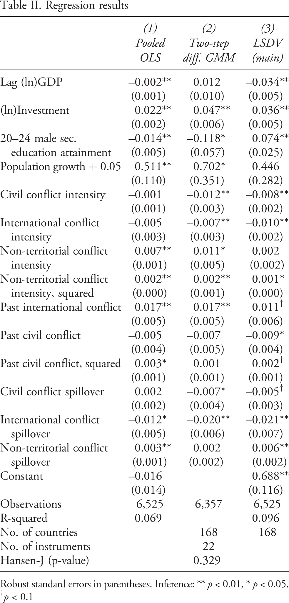
Robust standard errors in parentheses. Inference: ** p < 0.01, * p < 0.05, ^† p < 0.1

can be taken as evidence that conflict-affected countries benefit from the previously described phoenix effect. This is further supported by the fact that past international conflict and the squared intensity of past civil conflict are found to be positive and strongly significant.

Interestingly, a highly significant quadratic relationship is found for countries participating in conflicts on foreign soil. Thus, high levels of non-territorial conflict intensity seem to provide a Keynesian stimulus to growth (Reitschuler & Loening, 2005), while lower

Figure 3.

Association between conflict and growth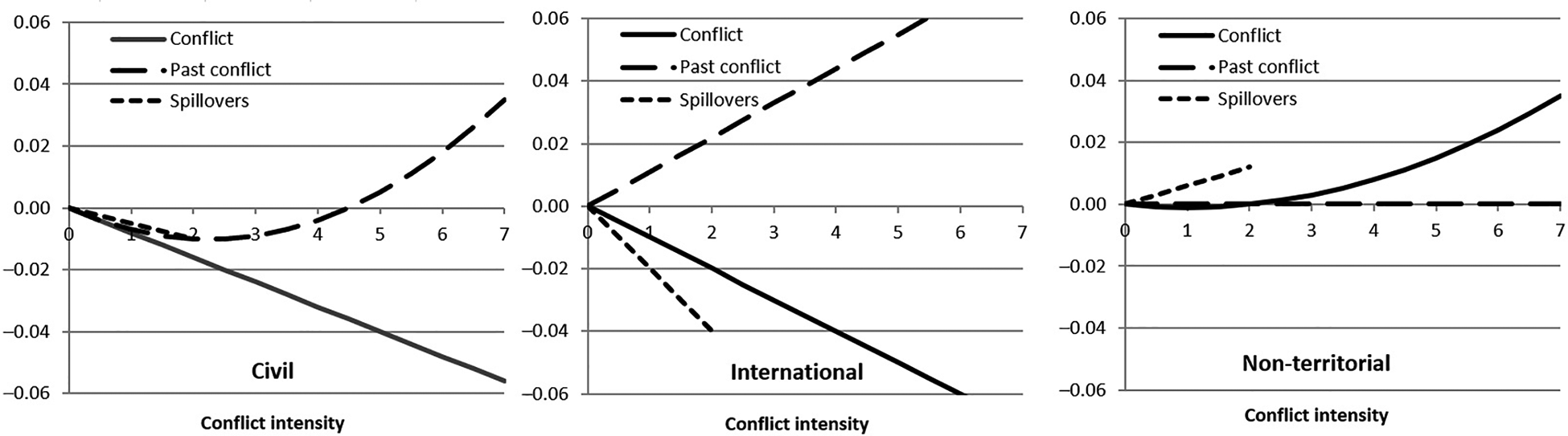

levels do not, thereby giving credence to Proposition 2. A possible explanation is that, with low-intensity conflict, the benefits from sending troops to a conflict on foreign soil might not be so clearcut, and thus the human, economic and social costs attributed to this military intervention could be higher. On the other hand, the spillover estimates show that those participants’ neighbours benefit from their involvement, while neighbours of an international conflict zone are shown to suffer significantly. As suggested by de Groot (2010), the latter finding is possibly due to the fact that neighbouring countries might not receive aid like ‘host’ countries do, if they are not seen as conflict victims by the international community. The former result, on the other hand, is likely explained by trade benefits, especially in the armament industry. These results provide some evidence for Proposition 3.

Consistent with our expectations that the within estimator has at most a small Nickell bias, the two-step difference GMM estimates (Column 2) are very similar to our preferred LSDV specification (Column 3). Although the Hansen-J test of over-identifying restrictions shows a p-value of 0.338, thereby not rejecting the hypothesis of instrument validity, the fact that it is above 0.25 hints at a potential instrument overproliferation issue (Roodman, 2009a), even after capping the number of instruments.

We thus concentrate on Column 3 for our short-run analysis. All the significant long-run results found in Column 1 are confirmed in this setting. On top of this, current civil and international conflicts are found to have a significant negative correlation with growth, which is consistent with Proposition 1. Our results show that, ceteris paribus, an additional intensity unit in a civil or international conflict leads to an average decrease of 0.8% or 1% of current GDP growth, respectively. Further supporting Proposition 3, the spillovers of both international and civil conflicts follow a negative linear trend while, again, a positive influence is observed on domestic growth when neighbouring states take part in non-territorial conflict.

We also find a significant quadratic relationship between past civil conflicts and growth. Hence, the latter is depressed following low-intensity conflicts and boosted after intense ones, thereby supporting Proposition 4. Thus, as suggested by Collier (1999) and corroborated by Gil-Alana & Singh (2015), the legacy of civil conflict seems to depend on the severity of conflict. We graphically summarize the conflict coefficient findings in Figure 3.

Robustness of regression results

In this section, we discuss the robustness of the relationships found in the regression analysis. All results are presented in the Online appendix A, Tables A.I–V.

Multicollinearity

In order to decide whether a strong multicollinearity bias emerges from including the Solow covariates with the conflict variables, we re-run the LSDV analysis, first excluding all conflict variables and then excluding all Solow covariates. Columns 2 and 3 in Table A.I in the Online appendix show that in both cases, the coefficients remain comparable to the main specification, both quantitatively and qualitatively. The same conclusion is found in Column 4, when using lagged Solow controls (which should not be impacted by current conflicts) instead of current ones in the main regression. Multicollinearity therefore does not seem to be a heavy threat.

Other specifications

First, to accommodate the possibility of global-wide shocks, we experiment using time-fixed effects. Second, as an omitted variable bias could emerge from not considering the quality of institutions, which can affect both growth and conflict intensity, we control for polity. This specification stays in the robustness section, however, as no data are available for ten of our observed countries. Third, we change our dependent variable to GDP level and to per capita GDP growth. Finally, we use different data sources for investment (World Bank, 2017) and education (Barro & Lee, 2013; Lutz et al., 2007; Samir et al., 2010). For the latter, we change the measure to the percentage of 15–64-year-olds with some secondary education (instead of focusing on the 20–24-year-old male population). Reassuringly, the previously found relationships are not affected by any of those alternatives (see Tables A.II–A.III).

Reverse causality

Our within-country methodology reduces the possibility that results may be driven by violent conflicts in traditionally low-growth countries. However, there might still be a concern that those countries are more likely to experience intense conflicts. Following Bircan, Brück & Vothknecht (2017), we thus replicate our results, this time splitting our sample into low- and high-growth groups. This is done by using the average quartile position of each country over the 45 years of observation, and then separating the countries between those whose average position was 1 or 2 (low growth), and those whose position was 3 or 4 (high growth).

Column 2 in Table A.IV shows the estimates when the sample is restricted to low-growth countries, while Column 3 shows the estimates for high-growth countries. Coefficients remain generally comparable in sign and significance across both subsamples, thereby assuaging concerns over reverse causality.

Geographical disparity

In order to decipher which countries seem to have the bigger weight on the regression results, we rerun the growth regressions, removing one region at a time. Results are presented in Table A.V in the Online appendix.

Current civil and international conflicts remain significant at the 1% level in all specifications. Europe, however, seems to drive the current non-territorial conflict results, which is unsurprising given its extensive participation in conflicts on foreign soil (see Figure 2). Meanwhile, Africa drives the post-civil conflict U-shaped correlation with growth, while Asia seems to have benefited the most strongly from a positive post-international conflict growth. However, the sign and magnitude of all these coefficients remain comparable across all specifications, which once again reassures us in our methodological choice.

Figure 4.

Confidence interval based on Monte Carlo methodology of parameter consistency

Counterfactual analysis

Our next step is to estimate a series of counterfactual annual GDP growth rates by subtracting the previously found conflict ‘effects’ from the actual yearly growth rates. These yearly counterfactual growth rates are then used to calculate counterfactual GDP levels, from which the true GDP outcomes are subtracted to estimate the yearly GDP gap due to conflict for each country.

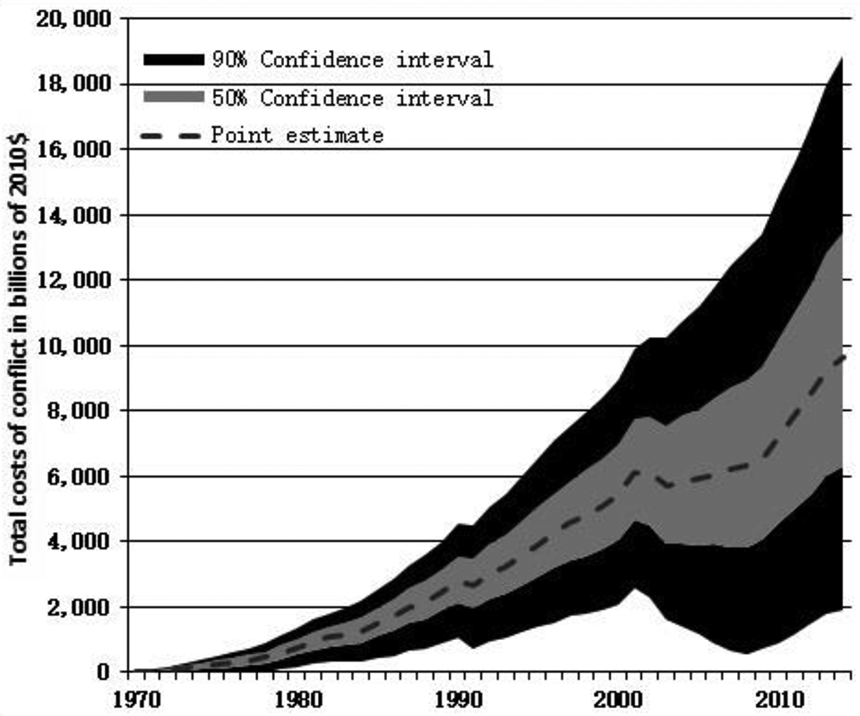
By 2014, we find that global GDP would have been 9.7 trillion 2010 US$ (or Tr$) larger if violent conflict had been absent since 1970, equalling 12.2% of global GDP. This net global cost estimate consists of gross costs of 12 Tr$ and gross benefits of 2.3 Tr$. A Monte Carlo estimation shows that the 90% confidence interval of our results yields costs between 1.9 and 18.9 Tr$ by 2014 (Figure 4).⁷

Results disaggregation

Differentiating our results across countries, we find that the influence of conflict varies significantly in relative terms (Figure 5A). For seven countries, total GDP would have more than doubled without violent conflict (Figure 5B). In absolute terms, China’s costs (3.3 Tr$) are the largest (Figure 5C), followed by India (1.6 Tr$) and Iraq (1.1 Tr$).

By region, Asia would have benefited the most from the absence of violent conflict between 1970 and 2014, whereas North America would have lost 0.9 Tr$ (Figure 5D). We generally find that developing countries

Figure 5.

Distribution and structure of the burden of violent conflict in 2014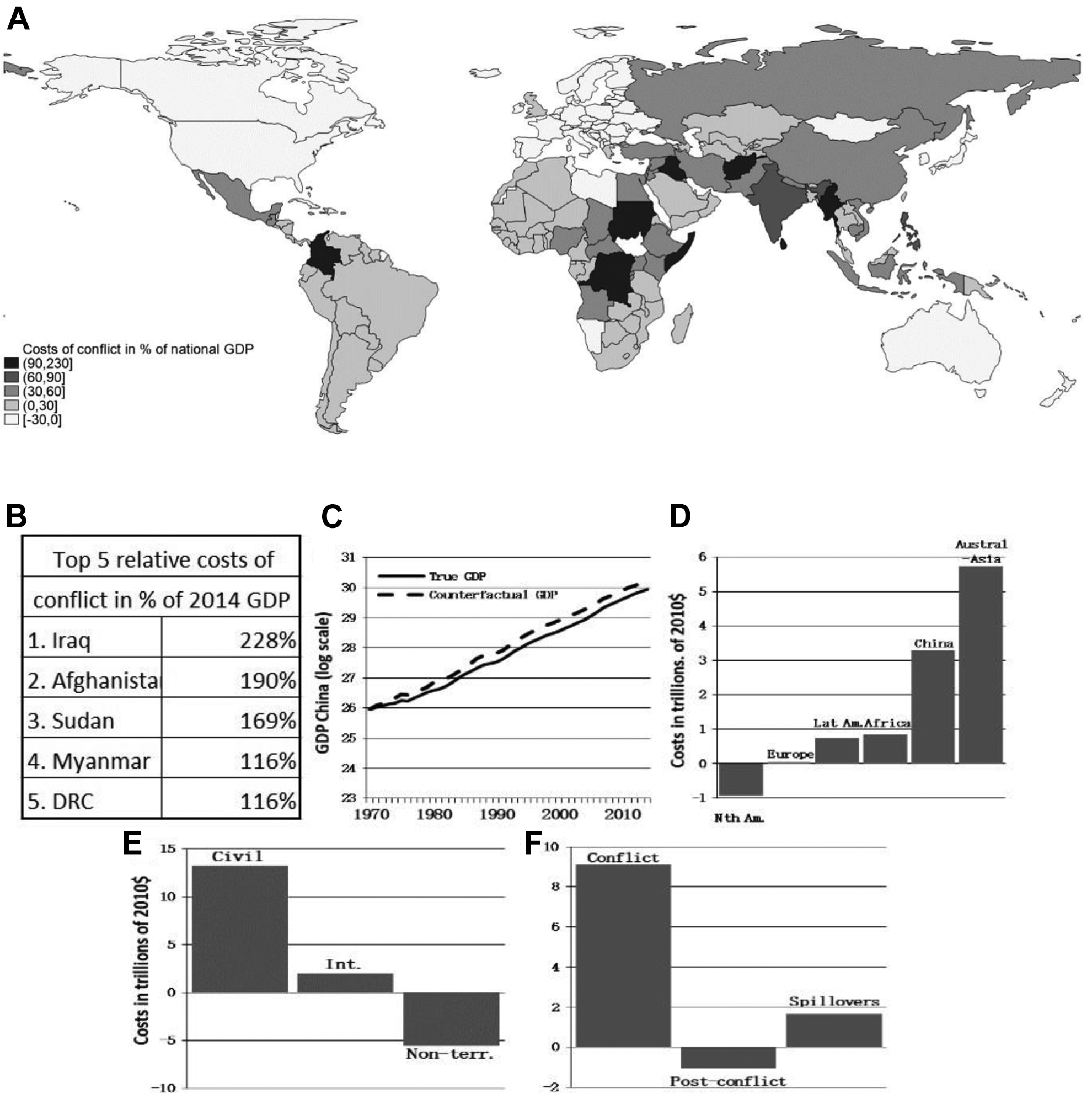

were economically harmed by conflict, while most high-income countries benefited from their participation in mainly non-territorial conflicts, thereby exaggerating global imbalances. This gap between poor and rich countries is also shown through the global cross-country Gini coefficient, which goes down from 0.641 to 0.634 in the absence of conflict. The decomposition across conflict types shows that civil conflict has by far the highest share of global conflict cost, while non-territorial conflicts reduce the net result (Figure 5E). Finally, Figure 5F shows that the highest share of global GDP loss from conflict stems from conflicts experienced within a country’s own territory (9.1 Tr$). Spillovers from neighbouring conflicts also lead to significant losses (1.7 Tr$), while accelerated post-conflict growth leads to a reduction of net costs (by 1.1 Tr$).

Figure 6.

Relevance of the global burden of conflict in a larger perspective

Sensitivity analysis

To test the sensitivity of our main result, we rerun our counterfactual analysis using four different specifications. Each approach yields broadly similar findings in terms of total costs, thereby confirming the robustness of our approach.

First, we re-run the cost estimation, this time including past non-territorial conflicts, the only conflict variable that had failed the double Lasso variable selection test. This merely reduces the conflict burden to 11.9% of 2014 global GDP. Second, we rerun the analysis, this time including time-fixed effects. Results increase slightly, to 14.5% of 2014 global GDP. Third, we move our window of 45 years of observations from 1970–2014 to 1960–2004.⁸ As a result, the global burden of conflict amounts to 13% of 2004 global GDP. This provides further support to the stability of our estimation. Fourth, our conflict intensity measure is based on a scale from 0 to 10 and includes criteria like state capabilities and capital destruction. As those can be found to be endogenous to GDP growth, we rerun our analysis using data from Gleditsch et al. (2002) instead, which measures conflict intensity based on a dichotomous index that solely relates to the number of directly related deaths. The global estimate is reduced very slightly, to 11.8% of 2014 global GDP.

Discussion

Comparison with other costs of conflict analyses

We first compare our results with recent articles that used the synthetic control method (Abadie & Gardeazabal, 2003) to estimate the cost of civil war (Bove, Elia & Smith, 2017; Costalli, Moretti & Pischedda, 2017). We, however, change some specifications to make our estimates comparable, by: (i) keeping current civil conflict as the sole conflict variable; (ii) changing our dependent variable to per capita GDP growth; and (iii) restricting the country-year sample selection to match each article. Restricting our sample to the 20 countries observed by Costalli, Moretti & Pischedda (2017), we find that a country loses, on average, 15.7% of its potential GDP per capita during the war-torn years. This is within the range between their original finding of 17.5%, and Bove, Elia & Smith’s (2017) replication of 12.8%. Next, when restricting our sample to the 27 countries observed by the latter article for their main result, our estimate is 9.9%, which is close to their 9.1% finding. These estimates are also in the same order of magnitude as Gates et al. (2012), who find that a median-size conflict decreases GDP per capita by 15%, and Mueller (2012), who finds a persistent loss of roughly 18% of GDP per capita caused by ongoing civil wars. These comparisons indicate that our approach produces plausible cost estimates.

Comparison with other global public bads

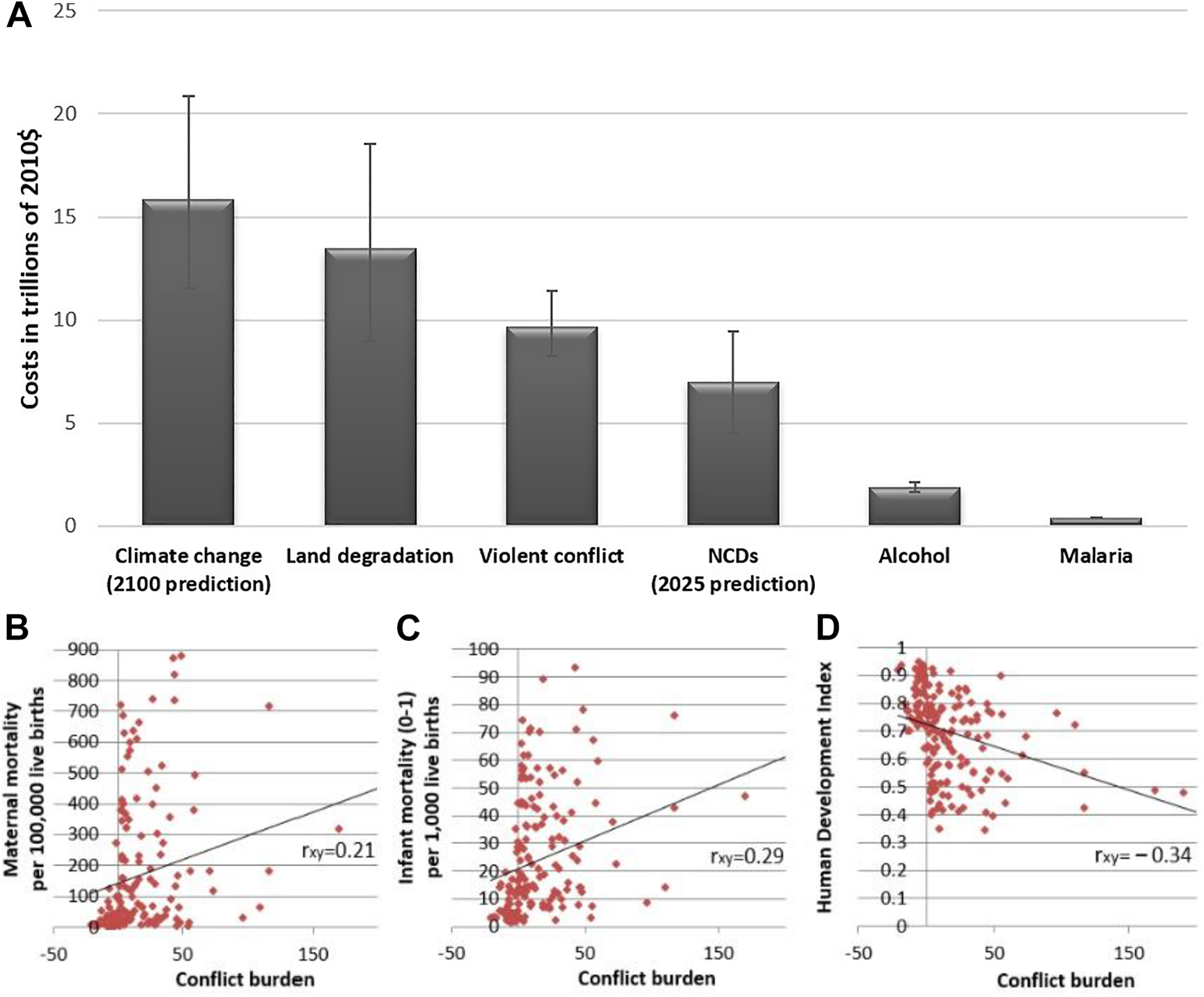
Figure 6A gives an indicative comparison of our result with the global burden of other public bads, based on various analyses. While methodologies, periods and country samples differ across studies, we adjusted each result to our setting as far as possible. A detailed explanation of this adjustment is provided in Online appendix B.

Our estimate of the global burden of violent conflict is found to be lower than that of climate change (Stern, 2007) and land degradation (ELD, 2015), but higher than non-communicable diseases (NCDs)⁹ (Bloom et al., 2011), alcohol consumption (Rehm et al., 2009) and malaria (Sachs & Malaney, 2002).

Comparison with other development indicators

Our results can be interpreted as the economic burden of conflict indicator (EBCI), measuring the accumulated GDP loss due to violent conflict across countries each

Figure 7.

Effects of different policy simulations on the global burden of conflict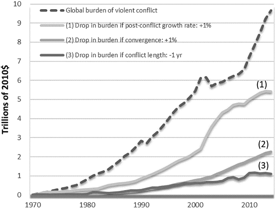

year. The 2014 EBCI correlates with other common indicators of socio-economic and health outcomes, including maternal and infant mortality and the human development index (Figures 6B–D). These results corroborate Gates et al. (2012), who find that conflict has detrimental effects on the reduction of poverty, hunger and child mortality. Our findings are hence further evidence that the sustainable development goals are negatively correlated with violent conflict.

Policy simulations

So far, our counterfactual estimations assumed that violent conflict is abolished entirely, which is clearly not a realistic policy option. Thus, we simulate some more nuanced policies, namely a reduction in the length of violent conflict (investments in peacebuilding) and increases in post-conflict growth (investments in reconstruction). Scenario 3 in Figure 7 shows that a one-year reduction in the length of all violent conflicts strongly reduces the burden of conflict. Likewise, an increase of one percentage point (pp) in the post-conflict rate of convergence term would help mitigate the GDP loss (scenario 2). However, the highest drop in the global burden of conflict is found when growth is increased by 1 pp for two years (for international conflicts) and four years (for civil conflicts) once conflict ends (scenario 1). Thus, the results show that one prominent way to reduce the burden of violent conflict is to rapidly invest in reconstruction after peace is achieved.

Conclusion

We find that, in 2014, the world would have been approximately 12% wealthier in the absence of violent conflict since 1970. Estimating the conflict-induced global GDP loss over a 45-year period gives valuable insights into the structure of the economic burden of violent conflict. Geographically, Asia is found to have suffered the largest accumulated costs, which were mostly driven by civil conflicts. On the other hand, North American, European, and Oceanic countries mainly benefited from their participation in conflicts which mostly occurred on foreign soil. This result helps explain not only the persistence of conflict but also the increasing trend in internationalized internal conflict.

We identify evidence of a ‘peace dividend’ in terms of higher growth in the post-conflict period. However, the net accumulated GDP gap due to conflict remains negative for most affected countries, especially those that experienced intense civil conflicts. Significant losses are even found for the peaceful neighbours of conflict-affected countries. These results thus underscore the need for the international community to make additional efforts regarding conflict resolution and peacekeeping. Comparing various policy solutions, we find that speeding up growth in the two to four years following the end of the conflict is a promising way to reduce the burden of violent conflict.

One important caveat to our work is that we do not estimate the costs of preventing conflict. However, while these costs may be high in the short run or may not always bear fruit, governments and international organizations alike should recognize that such an investment is crucial with a long-run perspective. One must, after all, compare the one-off cost of preventing a conflict to the continuous stream of future losses resulting from its onset.

Finally, we demonstrate that the global burden of violent conflict is comparable to the global burden of other public bads, such as climate change and diseases. We posit that these non-economic barriers to economic growth have been underappreciated, if not literally underestimated, by economists and political scientists alike. Global GDP growth can be stimulated in many ways; making peace clearly is one of them.

Footnotes

Replication data

Replication scripts and data can be found at . All analyses were conducted using Stata 15.1 and Excel 2016.

Acknowledgements

We thank Michael Brzoska, Joshua Catalano, Lisa Chauvet, Peter Croll, Valpy FitzGerald, Javier Gardeazabal, Paula Gobbi, Scott Gates, Gregory Hess, Debarati Guha-Sapir, Katharina Meidert, Matthew Minor, Håvard Nygård, Lutz Sager, Kati Krähnert, Gerald Schneider, Anja Shortland, Elisabeth Sköns, Christian Staacke, Felipe Valencia, Fedor van Rijn, Philip Verwimp, Sebastian Wolf and conference and seminar participants in Montreal, London, Berlin, Washington, DC, Stockholm, Amsterdam, Izmir, Brussels and Vancouver for their useful comments.

Funding

The authors acknowledge support from the German Foundation for Peace Research (DSF) through the Global Economic Costs of Conflict project.

ORCID iDs

Olaf J de Groot

Anousheh Alamir

Tilman Brück

Notes

References

Abadie

Alberto

Gardeazabal

Javier

(2003) The economic costs of conflict: A case study of the Basque Country. American Economic Review 93: 113–132.

Abadie

Alberto

Diamond

Alexis

Hainmueller

Jens

(2015) Comparative politics and the synthetic control method. American Journal of Political Science 59(2): 495–510.

Ahrens

Achim

Hansen

Christian B

Schaffer

Mark E

(2018) Pdslasso and ivlasso: Programs for post-selection and post-regularization OLS or IV estimation and inference. Statistical Software Components, Boston College Department of Economics (http://ideas.repec.org/c/boc/bocode/s458459.html).

Alvarez

Javier

Arellano

Manuel

(2003) The time series and cross-section asymptotics of dynamic panel data estimators. Econometrica 71(4): 1121–1159.

Anselin

Luc

(1988) Spatial Econometrics: Methods and Models. Vol. 4. Boston, MA: Kluwer Academic.

Arellano

Manuel

Bond

Stephen

(1991) Some tests of specification for panel data: Monte Carlo evidence and an application to employment equations. Review of Economic Studies 58(2): 277–297.

Aydin

Aysegul

(2012) Foreign Powers and Intervention in Armed Conflict. Palo Alto, CA: Stanford University Press.

Barro

Robert

Lee

Jong-Wha

(2013) A new data set of educational attainment in the world, 1950–2010. Journal of Development Economics 104(C): 184–198.

Barro

Robert J

Sala-i-Martin

Xavier

(1992) Convergence. Journal of Political Economy 100(2): 223–251.

10.

Belloni

Alexandre

Chernozhukov

Victor

Hansen

Christian

(2014) Inference on treatment effects after selection among high-dimensional controls. Review of Economic Studies 81(2): 608–650.

11.

Bircan

Cagatay

Brück

Tilman

Vothknecht

Marc

(2017) Violent conflict and inequality. Oxford Development Studies 45(2): 125–144.

12.

Blattman

Christopher

Miguel

Edward

(2010) Civil war. Journal of Economic Literature 48(1): 3–57.

13.

Blomberg

S Brock

Hess

Gregory D

(2006) How much does violence tax trade? Review of Economics and Statistics 88(4): 599–612.

14.

Blomberg

S Brock

Hess

Gregory D

Orphanides

Athanasios

(2004) The macroeconomic consequences of terrorism. Journal of Monetary Economics 51(5): 1007–1032.

15.

Bloom

David E

Chisholm

Dan

Jané-Llopis

Eva

Prettner

Klaus

Stein

Adam

Feigl

Andrea

(2011) From burden to ‘best buys’: Reducing the economic impact of non-communicable diseases in low- and middle-income countries. World Health Organization and World Economic Forum Report (http://www.who.int/nmh/publications/best_buys_summary.pdf).

16.

Bove

Vincenzo

Deiana

Claudio

Nisticò

Roberto

(2018) Global arms trade and oil dependence. Journal of Law, Economics, and Organization 34(2): 272–299.

17.

Bove

Vincenzo

Elia

Leandro

Smith

Ron P

(2017) On the heterogeneous consequences of civil war. Oxford Economic Papers 69(3): 450–568.

18.

Bove

Vincenzo

Gleditsch

Kristian Skrede

Sekeris

Petros G

(2016) Oil above water: Economic interdependence and third-party intervention. Journal of Conflict Resolution 60(7): 1251–1277.

19.

Bozzoli

Carlos

Brück

Tilman

(2009) Agriculture, poverty and post-war reconstruction: Micro-level evidence from Northern Mozambique. Journal of Peace Research 46(3): 377–397.

20.

Bozzoli

Carlos

Brück

Tilman

Sottsas

Simon

(2010) A survey of the global economic costs of conflict. Defence and Peace Economics 21(2): 165–176.

21.

Brück

Tilman

Di Maio

Michele

Miaari

Sami H

(2018) Learning the hard way: The effect of violent conflict on student academic achievement. Journal of the European Economic Association 17(5): 1502–1537.

22.

Calì

Massimiliano

Harake

Wissam

Hassan

Fadi

Struck

Clemens Christian

(2015) The impact of the Syrian conflict on Lebanese trade. Washington, DC, World Bank Group (https://openknowledge.worldbank.org/handle/10986/21914).

23.

Cerra

Valerie

Saxena

Sweta Chaman

(2008) Growth dynamics: The myth of economic recovery. American Economic Review 98(1): 439–457.

24.

Chang

Yang-Ming

Potter

Joel

Sanders

Shane

(2007) War and peace: Third-party intervention in conflict. European Journal of Political Economy 23(4): 954–974.

25.

Chen

Siyan

Loayza

Norman V

Reynal-Querol

Marta

(2008) The aftermath of civil war. World Bank Economic Review 22(1): 63–85.

26.

Choi

Seung-Whan

Salehyan

Idean

(2013) No good deed goes unpunished: Refugees, humanitarian aid, and terrorism. Conflict Management and Peace Science 30(1): 53–75.

27.

Collier

Paul

(1999) On the economic consequences of civil war. Oxford Economic Papers 51(1): 168–183.

28.

Collier

Paul

Elliott

Lani

Hegre

Håvard

Hoeffler

Anke

Reynal-Querol

Marta

Sambanis

Nicholas

(2003) Breaking the Conflict Trap: Civil War and Development Policy. Washington, DC: World Bank.

29.

Costalli

Stefano

Moretti

Luigi

Pischedda

Costantino

(2017) The economic costs of civil war: Synthetic counterfactual evidence and the effects of ethnic fractionalization. Journal of Peace Research 54(1): 80–89.

30.

Cramer

Christopher

(2007) Civil War Is Not a Stupid Thing: Accounting for Violence in Developing Countries. London: Hurst.

31.

de Groot

Olaf J

(2010) The spillover effects of conflict on economic growth in neighbouring countries in Africa. Defence and Peace Economics 21(2): 149–164.

32.

Dunne

John Paul

Tian

Nan

(2014) Conflict spillovers and growth in Africa. Peace Economics, Peace Science and Public Policy 20(4): 539–549.

33.

Dunne

John Paul

Tian

Nan

(2017) Legacies of civil wars: The long-term health costs after the fighting ends. Centre for the Study of African Economies, Conference, Oxford University (https://editorialexpress.com/cgi-bin/conference/download.cgi?db_name=CSAE2017&paper_id=632).

34.

Edwards

Ryan D

(2013) US war costs: Two parts temporary, one part permanent. Journal of Public Economics 113(C): 54–66.

35.

ELD Initiative (2015) The value of land: Prosperous lands and positive rewards through sustainable land management (https://www.eld-initiative.org/fileadmin/pdf/ELD-main-report_en_10_web_72dpi.pdf).

36.

Fearon

James D

Laitin

David

(2003) Ethnicity, insurgency and civil war. American Political Science Review 97(1): 75–90.

37.

Feenstra

Robert C

Inklaar

Robert

Timmer

Marcel P

(2015) The next generation of the Penn World Table. American Economic Review 105(10): 3150–3182.

38.

Fernandes

Nuno

(2020) Economic effects of coronavirus outbreak (COVID-19) on the world economy (https://ssrn.com/abstract=3557504).

39.

Gates

Scott

Hegre

Håvard

Nygård

Håvard Mokleiv

Strand

Håvard

(2012) Development consequences of armed conflict. World Development 40(9): 1713–1722.

40.

Gentle

James E

(1998) Random Number Generation and Monte Carlo Methods. New York: Springer.

41.

Gil-Alana

Luis A

Singh

Prakarsh

(2015) Growth recovery after civil conflict: A fractional integration approach. Defence and Peace Economics 27(4): 453–479.

42.

Gleditsch

Nils Petter

Wallensteen

Peter

Eriksson

Mikael

Sollenberg

Margareta

Strand

Håvard

(2002) Armed conflict 1946–2001: A new dataset. Journal of Peace Research 39(5): 615–637.

43.

Hegre

Håvard

Karlsen

Joakim

Nygård

Håvard Mokleiv

Strand

Håvard

Urdal

Henrik

(2013) Predicting armed conflict, 2010–2050. International Studies Quarterly 57(2): 250–270.

44.

Hendrix

Cullen S

Glaser

Sarah M

(2011) Civil conflict and world fisheries, 1953–2004. Journal of Peace Research 48(4): 481–495.

45.

Hoeffler

Anke

(2012) Armed conflict. Copenhagen Consensus Perspective Paper (http://www.copenhagenconsensus.com/sites/default/files/armedconflicts_perspective_1.pdf).

46.

House of Representatives Hearing (2010) The true cost of the war. Serial 111–103 (https://www.gpo.gov/fdsys/pkg/CHRG-111hhrg61761/pdf/CHRG-111hhrg61761.pdf).

47.

Hsiang

Solomon M

Jina

Amir S

(2014) The causal effect of environmental catastrophe on long-run economic growth: Evidence from 6,700 cyclones. NBER working paper 20352 (http://www.nber.org/papers/w20352).

48.

Inklaar

Robert

de Guevara

Juan Fernandez

Maudos

Joaquin

(2012) The impact of the financial crisis on financial integration, growth and investment. National Institute Economic Review 220(1): 29–35.

49.

Institute for Economics and Peace (IEP) (2016) The economic value of peace 2016 (https://www.visionofhumanity.org/wp-content/uploads/2020/10/The-Economic-Value-of-Peace-2016-WEB.pdf).

50.

Kalkuhl

Matthias

Wenz

Leonie

(2020) The impact of climate conditions on economic production. Evidence from a global panel of regions. Journal of Environmental Economics and Management 103: 102360 (https://doi.org/10.1016/j.jeem.2020.102360).

51.

Kang

Seonjou

Meernik

James

(2005) Civil war destruction and the prospects for economic growth. Journal of Politics 67(1): 88–109.

52.

Keynes

John Maynard

(1920) The Economic Consequences of the Peace. Vol. 178. London: Macmillan.

53.

Knight

Malcolm

Loayza

Norman

Villanueva

Delano

(1996) The peace dividend: Military spending cuts and economic growth. World Bank policy research working paper 1577 (http://documents.worldbank.org/curated/en/154941468766463442/The-peace-dividend-military-spending-cuts-and-economic-growth).

54.

Lai

Brian

Thyne

Clayton

(2007) The effect of civil war on education, 1980–97. Journal of Peace Research 44(3): 277–292.

55.

Larsen

Bjorn

(2014) Benefits and costs of the air pollution targets for the post-2015 development agenda. Post-2015 Consensus air pollution assessment paper (http://www.copenhagenconsensus.com/sites/default/files/air_pollution_assessment_-_larsen.pdf).

56.

Lind

Jo Thori

Mehlum

Halvor

(2010) With or without U? The appropriate test for a U-shaped relationship. Oxford Bulletin of Economics and Statistics 72(1): 109–118.

57.

Lutz

Wolfgang

Goujon

Anne

Samir

Sanderson

Warren

(2007) Reconstruction of Population by Age, Sex and Level of Educational Attainment for 120 Countries 1970–2000. Laxenburg: IIASA (http://dataexplorer.wittgensteincentre.org/shiny/wic/).

58.

Mankiw

N Gregory

Romer

David

Weil

David N

(1992) A contribution to the empirics of economic growth. Quarterly Journal of Economics 107(2): 407–437.

59.

Manski

Charles F

(1993) Identification of endogenous social effects: The reflection problem. Review of Economic Studies 60(3): 531–542.

60.

Marshall

Monty G

Cole

Benjamin R

(2014) Global report 2014: Conflict, governance, and state fragility. Center for Systemic Peace, Vienna, VA (https://www.researchgate.net/publication/265905476_Global_Report_2014_Conflict_Governance_and_State_Fragility).

61.

Marshall

Monty G

Gurr

Ted Robert

Jaggers

Keith

(2017) Polity IV Project: Political regime characteristics and transitions, 1800–2017 (http://www.systemicpeace.org/inscrdata.html).

62.

McKibbin

Warwick J

Fernando

Roshen

(2020) The global macroeconomic impacts of COVID-19: Seven scenarios. CAMA working paper 19 (https://ssrn.com/abstract=3547729).

63.

Miguel

Edward

Roland

Gérard

(2011) The long-run impact of bombing Vietnam. Journal of Development Economics 96(1): 1–15.

64.

Miguel

Edward

Satyanath

Shanker

Sergenti

Ernest

(2004) Economic shocks and civil conflict. Journal of Political Economy 112(4): 725–753.

65.

Montalvo

Jose G

Reynal-Querol

Marta

(2007) Fighting against malaria: Prevent wars while waiting for the ‘miraculous’ vaccine. Review of Economics and Statistics 89(1): 165–177.

66.

Mueller

Hannes

(2012) Growth dynamics: The myth of economic recovery: Comment. American Economic Review 102(7): 3774–3777.

67.

Mueller

Hannes

(2013) The economic costs of conflict. IGC working paper (http://www.theigc.org/wp-content/uploads/2014/09/Mueller-2013-Working-Paper2.pdf).

68.

Murdoch

James C

Sandler

Todd

(2002a) Economic growth, civil wars and spatial spillovers. Journal of Conflict Resolution 46(1): 91–110.

69.

Murdoch

James C

Sandler

Todd

(2002b) Civil wars and economic growth: A regional comparison. Defense and Peace Economics 13(6): 451–464.

70.

Murdoch

James C

Sandler

Todd

(2004) Civil wars and economic growth: Spatial dispersion. American Journal of Political Science 48(1): 138–151.

71.

Nickell

Stephen

(1981) Biases in dynamic models with fixed effects. Econometrica 49(6): 1417–1426.

72.

Office for the Coordination of Humanitarian Affairs (OCHA) (2017) World humanitarian data and trends 2017 (https://interactive.unocha.org/publication/datatrends2017/resources/WHDT2017_Final_Singles.pdf).

73.

Olson

Mancur

(1982) The Rise and Decline of Nations. New Haven, CT: Yale University Press.

74.

Organski

AFK

Kugler

Jacek

(1977) The costs of major wars: The phoenix factor. American Political Science Review 71(4): 1347–1366.

75.

Pimentel

David

Harvey

Celia

Resosudarmo

Pradnja

Sinclair

Kurz

McNair

Crist

Shpritz

Fitton

Saffouri

(1995) Environmental and economic costs of soil erosion and conservation benefits. Science-AAAS-Weekly Paper Edition 267(5201): 1117–1122.

76.

Polacheck

Solomon W

Sevastianova

Daria

(2012) Does conflict disrupt growth? Evidence of the relationship between political instability and national economic performance. Journal of International Trade and Economic Development 21(3): 361–388.

77.

Rehm

Jürgen

Mathers

Colin

Popova

Svetlana

Thavorncharoensap

Montarat

Teerawattananon

Yot

Patra

Jayadeep

(2009) Global burden of disease and injury and economic cost attributable to alcohol use and alcohol-use disorders. Lancet 373(9682): 2223–2233.

78.

Reitschuler

Gerhard

Loening

Josef L

(2005) Modeling the defense–growth nexus in Guatemala. World Development 33(3): 513–526.

79.

Roodman

David

(2009a) A note on the theme of too many instruments. Oxford Bulletin of Economics and Statistics 71(1): 135–158.

80.

Roodman

David

(2009b) How to do xtabond2: An introduction to difference and system GMM in Stata. Stata Journal 9(1): 86–136.

81.

Sachs

Jeffrey

Malaney

Pia

(2002) The economic and social burden of malaria. Nature 415(6872): 680–685.

82.

Salehyan

Idean

Gleditsch

Kristian Skrede

(2006) Refugees and the spread of civil war. International Organization 60: 335–366.

83.

Samir

Barakat

Bilal

Goujon

Anne

Skirbekk

Vegard

Sanderson

Warren

Lutz

Wolfgang

(2010) Projection of populations by level of educational attainment, age, and sex for 120 countries for 2005–2050. Demographic Research 22: 383–472.

84.

Serneels

Pieter

Verpoorten

Marijke

(2015) The impact of armed conflict on economic performance: Evidence from Rwanda. Journal of Conflict Resolution 59(4): 555–592.

85.

Slater

Dan

(2010) Ordering Power: Contentious Politics, State-Building, and Authoritarian Durability in Southeast Asia. Cambridge: Cambridge University Press.

86.

Smith

Ron P

(2014) The economic costs of military conflict. Journal of Peace Research 51(2): 245–256.

87.

Solow

Robert M

(1956) A contribution to the theory of economic growth. Quarterly Journal of Economics 70(1): 65–94.

88.

Stern

Nicholas H

(2007) The Economics of Climate Change: The Stern Review. Cambridge: Cambridge University Press.

89.

Stiglitz

Joseph E

Bilmes

Linda J

(2008) The Three Trillion Dollar War: The True Cost of the Iraq Conflict. New York: WW Norton.

90.

Unruh

Jon D

Heynen

Nikolas C

Hossler

Peter

(2003) The political ecology of recovery from armed conflict: The case of landmines in Mozambique. Political Geography 22(8): 841–861.

91.

Veenstra

Nina

Whiteside

Alan

(2005) Economic impact of HIV. Best Practice & Research Clinical Obstetrics & Gynaecology 19(2): 197–210.

92.

Verwimp

Philip

Justino

Patricia

Brück

Tilman

(2009) The analysis of conflict: A micro-level perspective. Journal of Peace Research 46(3): 307–314.

93.

Verwimp

Philip

Justino

Patricia

Brück

Tilman

(2019) The microeconomics of violent conflict. Journal of Development Economics 141: 102297 (https://doi.org/10.1016/j.jdeveco.2018.10.005).

94.

Weidmann

Nils B

Kuse

Doreen

Gleditsch

Kristian Skrede

(2010) The geography of the international system: The Cshapes dataset. International Interactions 36(1): 86–106.

95.

Weinstein

Jeremy

Imai

Kosuke

(2000) Measuring the economic impact of civil war. Center for International Development at Harvard University, CID working paper 051 (https://imai.princeton.edu/research/files/cid.pdf).

96.

World Bank (2017) World Development Indicators 2017. Washington, DC: World Bank.

97.

World Bank (2020) Violence without Borders: The Internationalization of Crime and Conflict. Policy Research Report. Washington, DC: World Bank.

98.

Yach

Derek

Stuckler

David

Brownell

Kelly D

(2006) Epidemiologic and economic consequences of the global epidemics of obesity and diabetes. Nature Medicine 12(1): 62–66.

The global economic burden of violent conflict

Abstract

Keywords

Introduction

Conceptual framework

Empirical model

Possible influences of conflict on economic growth

Current conflicts

Neighbouring conflicts

Past conflicts

Data and methods

Data sources and variables

Dependent variable

Current conflicts

Past conflicts

Neighbouring conflicts

Controls

Variable selection

Methodology

Challenges

Regression analysis

Counterfactual analysis

Results

Regression analysis

Robustness of regression results

Multicollinearity

Other specifications

Reverse causality

Geographical disparity

Counterfactual analysis

Results disaggregation

Sensitivity analysis

Discussion

Comparison with other costs of conflict analyses

Comparison with other global public bads

Comparison with other development indicators

Policy simulations

Conclusion

Footnotes

Replication data

Acknowledgements

Funding

ORCID iDs

Notes

References