Sage Journals: Discover world-class research

Abstract

This article presents an update to the ViEWS political Violence Early-Warning System. This update introduces (1) a new infrastructure for training, evaluating, and weighting models that allows us to more optimally combine constituent models into ensembles, and (2) a number of new forecasting models that contribute to improve overall performance, in particular with respect to effectively classifying high- and low-risk cases. Our improved evaluation procedures allow us to develop models that specialize in either the immediate or the more distant future. We also present a formal, ‘retrospective’ evaluation of how well ViEWS has done since we started publishing our forecasts from July 2018 up to December 2019. Our metrics show that ViEWS is performing well when compared to previous out-of-sample forecasts for the 2015–17 period. Finally, we present our new forecasts for the January 2020–December 2022 period. We continue to predict a near-constant situation of conflict in Nigeria, Somalia, and DRC, but see some signs of decreased risk in Cameroon and Mozambique.

Keywords

Africa armed conflict ensemble modeling forecasting model criticism

Overview

This article presents an update to the ViEWS political violence early-warning system first presented in Hegre et al., 2019. We outline improvements to a number of components: we have enhanced ViEWS’ ability to forecast conflict onsets and to separate low- and high-risk cases; we have made adjustments to the dependent variables to increase the usefulness of the system, improved the methodology, and expanded the set of predictors. We first summarize and motivate these changes, and proceed to show how these revisions improve performance. The revisions primarily pertain to forecasts at the country level. Changes to the subnational level have been more incremental, and we therefore allocate less space to these developments.

In line with ViEWS’ goal of maximal transparency, we also revisit ViEWS forecasts published in Hegre et al. (2019) and the monthly updates on the website (https://pcr.uu.se/research/views/current-forecasts/). The evaluation shows that overall predictive performance is in line with our expectations in Hegre et al. (2019). Finally, we summarize the new forecasts for the January 2020–December 2022 period.¹

Figure 1.

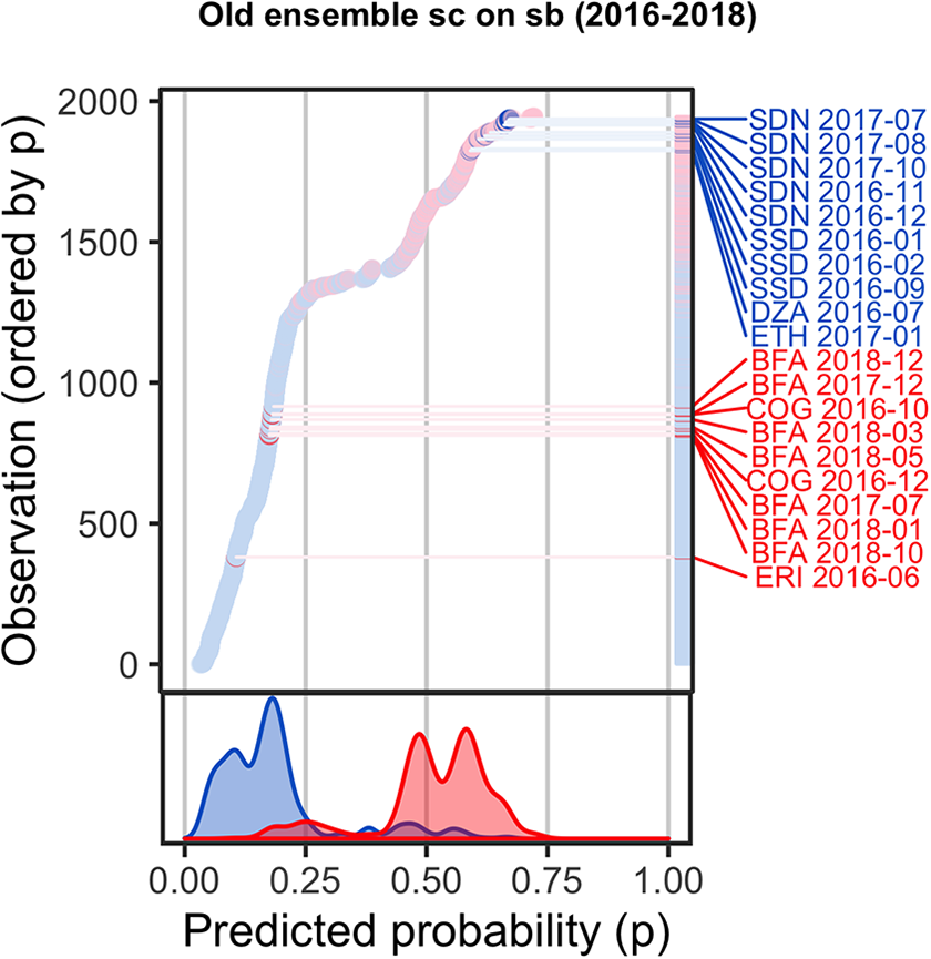
Model criticism of Hegre et al. (2019) cm ensemble, state-based conflict (2016–18)

Revising the ViEWS pilot

In Hegre et al. (2019) we indicated several potential avenues to strengthening the performance of the system, such as increasing the system’s ability to forecast political violence in countries with little pre-existing conflict and to separate between low- and high-risk cases. To highlight how the system presented in Hegre et al. (2019) fared with regard to these two dimensions, we make use of the model criticism plot in Figure 1 (Colaresi & Mahmood, 2017).²

The figure indicates that the ViEWS ensemble overestimated the risk of conflict continuation and underestimated the probability in hitherto peaceful countries. Some cases reflect these general patterns: the ensemble consistently predicted a high risk of conflict in Sudan in 2017–18 (shown as blue dots and labeled ‘SDN [date]’). The red labeled dots are instances where we assigned low risk to cases that did experience conflict. A number of these were countries without significant recent conflict before 2016 (e.g. Eritrea). As we detail below, we have sought to improve the ability of the system to capture early signs of violence even in absence of recent conflicts, as well as identify a decrease in conflict probability in locations with recent conflict history.

Second, while in Hegre et al. (2019) the ViEWS ensemble was calibrated so that the average predicted probability of conflict was close to the actual relative frequency, it did not separate well between low- and high-risk cases. This is clear from the marginal plot in Figure 1: very few observations had a predicted probability higher than 0.75 or lower than 0.05, and the red (positive cases) and blue (negative cases) densities overlap. This lack of separation was the result of incorporating a handful of overall poorly performing models in the ViEWS ensemble, and the lack of weighting. Below, we elaborate on how we revised the set of constituent models and improved our ensemble procedures to produce sharper forecasts.

Changes to how we handle data for model evaluation and averaging

We have improved the ViEWS system for handling data and out-of-sample evaluation. In the following, we will refer to a specification as a ‘model’ $m^{(j)}$ . When we use input data up to December 2015, we generate forecasts for each of the 36 months from January 2016 to December 2018. We refer to these as steps $s \in [1, 36]$ . We train each model specifically for each s. $m^{(j,1)}$ is trained to predict $s = 1$ month into the future, $m^{(j,6)}$ $s = 6$ months forward, and so on. As before, we split our data into three partitions (Table I). For each model $m^{(j)}$ and step $s \in [1, 36]$ , our procedure:

Trains model $m^{(j, s)}$ on monthly data in some range from $τ_{0}^{e}$ to $τ_{t}^{e}$ where $τ_{0}^{e}$ is the first observation available for training, and $τ_{t}^{e}$ is the last observation before the calibration period.

Generates predictions for all months i in the calibration period ( $τ_{t}^{e} + 1, τ_{c}^{e}$ ), using data up to s months before i.

Calibrates model, obtains ensemble weights, and tunes hyper-parameters using the predictions from (2) along with the actuals for all months in the calibration period.

Retrains model using both the training and calibration periods ( $τ_{0}, τ_{c}^{e}$ ).

Generates predictions for the testing/forecasting period ( $τ_{c}^{e} + 1, τ_{f}^{e}$ ).

Table I.

Partitioning of data for estimating model weights, hyper-parameter tuning, evaluation, and forecasting

	Periodization
	Evaluation	Forecast
Training period	$τ_{0}^{e} = 121$ (January 1990)	$τ_{0} = 121$ (January 1990)
	$τ_{t}^{e} = 396$ (December 2012)	$τ_{t} = 432$ (December 2015)
Calibration period	$τ_{t}^{e} + 1 = 397$ (January 2013)	$τ_{t} + 1 = 433$ (January 2016)
	$τ_{c}^{e} = 432$ (December 2015)	$τ_{c} = 468$ (December 2018)
Testing/forecasting	$τ_{c}^{e} + 1 = 433$ (January 2016)	$τ_{c} + k = 481$ (January 2020)
period	$τ_{f}^{e} = 468$ (December 2018)	$τ_{f} = 516$ (December 2022)

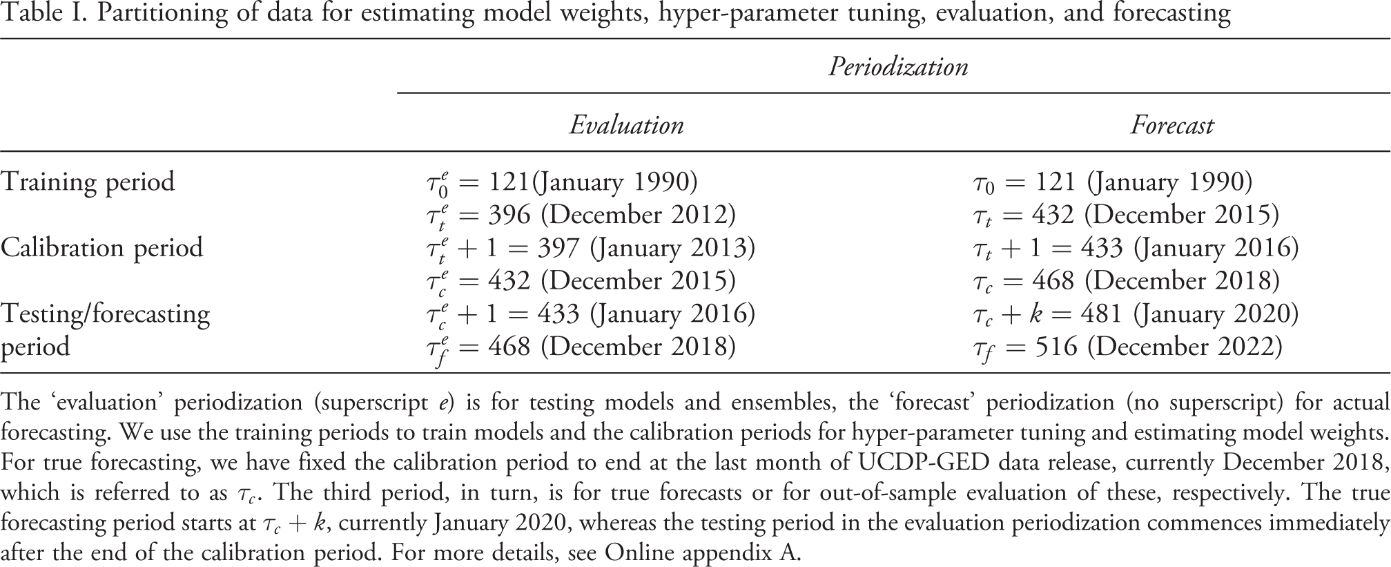
The ‘evaluation’ periodization (superscript e) is for testing models and ensembles, the ‘forecast’ periodization (no superscript) for actual forecasting. We use the training periods to train models and the calibration periods for hyper-parameter tuning and estimating model weights. 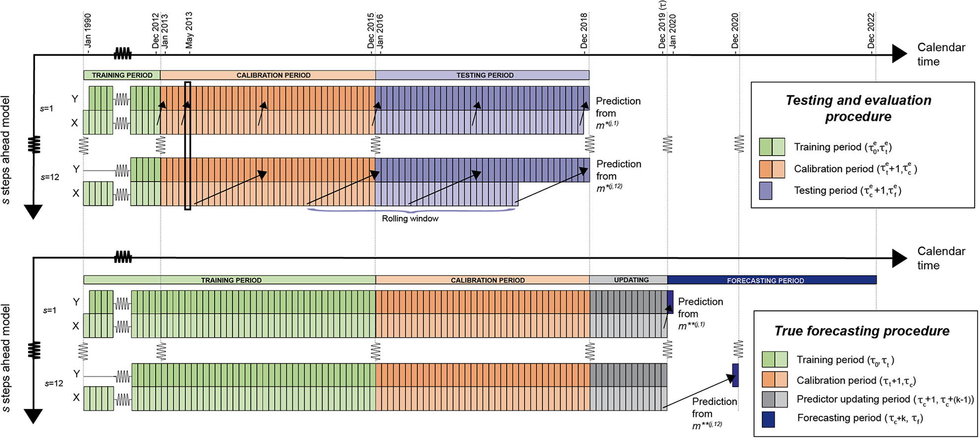For true forecasting, we have fixed the calibration period to end at the last month of UCDP-GED data release, currently December 2018, which is referred to as $τ_{c}$ . The third period, in turn, is for true forecasts or for out-of-sample evaluation of these, respectively. The true forecasting period starts at $τ_{c} + k$ , currently January 2020, whereas the testing period in the evaluation periodization commences immediately after the end of the calibration period. For more details, see Online appendix A.

Figure 2.

Management of temporal domain (timeshifting, periodization) in current pipeline, for evaluation (top) and forecasting (bottom)

In step 5, the procedure is different when we evaluate models than when we generate true forecasts. The two variants of the procedure are summarized in Figure 2 and described in more detail in Online appendix A. When evaluating the models, we generate predictions for each month in the testing period.We then match $s = 2$ forecasts for January 2016 (based on input data up to November 2015) with what actually happened in January 2016, $s = 2$ forecasts for February 2016 with actuals for February 2016, etc., for all s. This means that a model $m^{(j,2)}$ targeting $s = 2$ is evaluated against all 36 months in our calibration or testing period.

When we generate true forecasts, however, we only make forecasts based on the most recent input data. For the forecasts presented below, we have data up to December 2019. We make one set of forecasts at $s = 1$ for January 2020, one at $s = 2$ for February 2020, etc.

In Hegre et al. (2019), we used the current procedure for forecasts also when evaluating, calibrating, and estimating model weights. The new setup provides us with much more data for testing and calibration, enabling us to estimate ensemble weights more precisely and specifically for each s. We also have more data for hyper-parameter tuning, allowing us to introduce new algorithms. In addition, our evaluation of individual models in the ensemble yields more precise results, as we can allow similar model specifications to perform differently for different s. We now capture that some models are more important for forecasting the immediate future and others for the more distant ones.

Changes to dependent variables

We continue to generate predictions at the country-month (cm) and PRIO-GRID-month (pgm) levels for each of the UCDP forms of organized violence (state-based (sb), one-sided (os), or non-state (ns)) (Pettersson, Högbladh & Öberg, 2019). In Hegre et al. (2019), we defined the outcomes requiring only one battle-related death (BRD) per month at both the country and PRIO-GRID (Tollefsen, Strand & Buhaug, 2012) levels. At the cm level, we now require at least 25 BRDs. This more demanding threshold yields more relevant warnings.

We continue to use the single-death threshold for the PRIO-GRID unit of analysis, as the threshold of 25 BRDs is rarely surpassed within a month in an area as small as the ∼ 55x55 km PRIO-GRID cell. Also, we include models at the country level trained on the lower BRD threshold in our model ensemble, as they may provide useful indications on early signs of violence and thus contribute to identify conflict outbreaks.

Ensembles

The final forecasts in ViEWS are generated by combining models in ensembles.³ Ensembles can improve predictive performance and make predictions more robust to new data since a broader set of models are less sensitive to overfitting (Armstrong, 2001). In Hegre et al. (2019), our ensembles were unweighted model averages, as they did as well as the weighted ones. We have switched to ensemble Bayesian model averaging (EBMA; Montgomery, Hollenbach & Ward, 2012) at the cm level, since it now outperforms unweighted ensembles at the cm level.

EBMA performs better than unweighted averages since it allows including more models that specialize for subsets of the data in addition to broader ones. Such targeted models perform poorly in isolation. For example, the onset models we present below are poor at predicting conflict incidence, but incorporating them improves the anticipation of new or re-emerging conflicts. As we discussed above, these models can severely impact the ability of the unweighted ensemble to separate between low- and high-risk cases. Weighting each model’s impact on the ensemble by predictive performance solves this problem. EBMA now performs better since the new infrastructure provides us with more data for model weighting. Given this, we can relate observed outcomes Y for every month in the calibration period to predictions for every model $m^{(j, s)}$ at each step s, as compared to $m^{(j)}$ in the past. The weights are based on an increased number of observations and thus more accurate. At the pgm level, however, EBMA does not currently improve performance and we therefore continue to use unweighted model averages. Candidate explanations for why EBMA outperforms the unweighted ensemble at the cm but not at the pgm level include the quality and comprehensiveness of features and models, as well as severe class imbalance at the pgm level.

New set of constituent models

We have revised the set of constituent models in the cm and pgm ensembles considerably, in particular by weeding out poor models and improving the ability to anticipate conflict in more peaceful countries. We discuss the criteria for adding and retaining models below.

To simplify the organization, we use the same models for all steps and for all outcomes. Here, we illustrate the major changes compared to Hegre et al. (2019). More details are found in Online appendices B and C.

New models and data at cm level

The new cm level ensembles include 16 models (Figure 3). Most are trained by means of a random forest classifier algorithm (Breiman, 2001), implemented using the scikit-learn package (Pedregosa et al., 2011). For the random forest models, we set the number of trees to 1,000 and use package defaults otherwise. Details, feature importances, and prediction maps are found in Online appendix B.

We have sought to improve performance for new conflicts along two avenues. The first is to expand models that include ‘structural’, slow-changing factors that capture latent risks of conflict. Our theoretical expectation is that these should dominate forecasts a couple of years into the future, when the current immediate history is less important. The vdem_glob model includes variables describing countries’ political institutions from the Varieties of Democracy (V-Dem) dataset (Coppedge et al., 2017). The likelihood of conflict is highest for half-democracies and after recent regime change (Cederman, Hug & Krebs, 2010; Hegre et al., 2001). The wdi_all_glob model contains socio-economic indicators from the World Development Indicators (World Bank, 2019), ranging from poverty and health measures through indicators for inequality or the quality of

Figure 3.

Performance of constituent models (vertical axis), 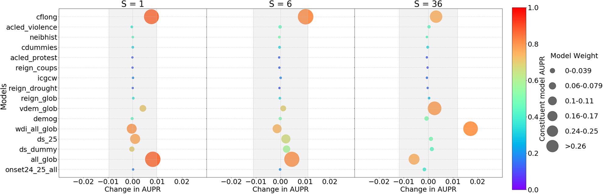sb, cm, for $s = 1$ (left panel), $s = 6$ (middle), $s = 36$ (right)

national policies (Hegre, 2018). We have retained the demog model from Hegre et al. (2019).

The second approach is to capture early signals of increasing tensions for short-term forecasts. Data for these models are updated monthly. The ACLED_protest and ACLED_violence models include recent history of protest and violence (Raleigh et al., 2010). The icgcw model uses monthly warnings from the International Crisis Group’s Crisis Watch (https://www.crisisgroup.org/crisiswatch). The reign_glob model incorporates information on recent elections, coups, and other leader changes and the reign_coups model contains the predicted risk of military coups, both sourced from the REIGN Dataset (Bell, 2016; www.oefresearch.org). These model escalation and dynamics of political violence related to transitions induced by coups (Belkin & Schofer, 2003) or elections (Birch, Daxecker & Höglund, 2020). The reign_drought model taps into early signals of tensions by including drought/precipitation data (von Uexkull et al., 2016).

We have amended our conflict history models in order to reduce the system’s tendency to overestimate risk in countries with recent conflict. The new, extensive cflong model contains detailed information of the severity of past violence in terms of the number of people killed and how much time has elapsed since earlier violence. We also have included a neibhist model that describes the conflict history of a country’s neighbors, building from the evidence that violence tends to spatially cluster (Gleditsch, 2002).

The ensembles also include a very broad random forest model all_glob, containing all the features described above, designed to capture interactive effects. Also using all features, onset_24_25_all is trained on onset of conflict rather than incidence, in an effort to improve the ensemble’s ability to predict the outbreak of violence.⁴

As in Hegre et al. (2019), we include two broad ‘dynamic simulation’ models that have the logistic regression model at its core. One of these (ds_dummy) is trained on the incidence of conflict with at least one battle-related death (BRD) as the outcome variable, the other (ds_25) using the incidence of at least 25 BRDs (see Online appendix B for details).

New models at pgm level

The new pgm level ensembles include 12 models based on subnational data (Tollefsen, Strand & Buhaug, 2012). The high spatial resolution of conflict predictors enables the pgm level models to better capture differences across space than cm models, indicating where conflicts are likely. As the risk of conflict can be influenced by both local and national factors, in the cross_level model, we also make the two levels of analysis inform each other. Unless otherwise noted, models were trained using random forests. Details, prediction maps, and feature importance are found in Online appendix C.

We have retained the pgd_natural, pgd_social and two dynamic simulation models (ds_dummy, ds_25) from Hegre et al. (2019). Our changes to the pgm level models have also aimed to improve ViEWS’ ability to predict conflict onset. The spei_full model measures the occurrence of droughts (Vicente- Serrano, Beguera & López-Moreno, 2010), which can push deprived communities to mobilize upon pre-existing grievances (von Uexkull et al., 2016). A new conflict history model called sptime seeks to discriminate better between low and high risk of violence. It contains features representing various relative weightings of spatial and temporal distance to conflict.

In addition, four broad models make use of all the features listed above. The allthemes model is trained on the incidence of conflict, and the onset24_100_all and onset24_1_all models are trained on two definitions of local onset to help predicting the first cases of violence.⁵ Finally, the xgb model applies the XGBoost gradient boosting decision tree algorithm (Chen & Guestrin, 2016) to all features. Five core hyper-parameters were tuned using a genetic algorithm (Russell & Norvig, 2016), where models were trained using an initial random sample of possible hyper-parameter combinations and scored based on the AUPR metric. In an iterative process resembling natural selection, the best-performing models pass on hyper-parameter values to further iterations while adding random ‘mutation’ to explore the parameter space. The final xgb model is an ensemble of the best five performing hyper-parameter sets in any iteration. More details on the procedure are given in Online appendix C.

Evaluation

Constituent models

There is no golden rule to establish which models to include in an ensemble. The most important criterion is that they improve predictive performance. Second, models should be interpretable on their own, as we discuss below (Figure 9). Finally, the more distinct the models in the ensemble, the larger the joint contribution, just as a crowd is wiser if there is diversity of opinion within it. Accordingly, our criterion for including or excluding the models in the ensemble is built in the spirit of Mill’s ‘harm principle’: we remove models if they harm the predictive performance of the ensemble in the test partition of the data. To avoid this decision being determined by random events in the test partition, we define ‘harm’ as reducing the AUPR of the ensemble by more than 0.5 standard errors, estimated by bootstrapping. We drew 100,000 samples of prediction–actual pairs from the full ensemble, computed the AUPR for each of these samples, and calculated the standard error as the standard deviation across the bootstrapped AUPR metrics. We then compared the difference in AUPR between the full ensemble and the reduced ensemble with the bootstrapped standard error of the AUPR for the full ensemble. All our models at the cm level passed this test.

Figure 3 summarizes the predictive performance of the constituent models and ensembles, for steps 1, 6, and 36 at the cm level. It reports the weight of the models in the ensemble, AUPR for the predictions from the individual models, and the extent to which they contribute to the predictive performance of the ensemble.⁶

Individual predictive performance varies greatly between models. For $s = 1$ , the red-colored circles representing the cflong and all_glob models show that they are better at picking up true positives (AUPR) than for instance the blueish onset_24_25_all. The sizes of their circles reflect their higher weight in the ensembles. These models are also most important to the ensemble as removing them reduces AUPR for the ensemble considerably, at least for short forecasting horizons ( $s = 1, 6$ ). When looking $s = 36$ months into the future, the wdi_all_glob – which includes more structural features – is most important.

Models that perform poorly, however, may still contribute important information to the ensemble predictions. The onset_24_25_all model performs poorly overall since most conflict observations in our data are already ongoing conflicts. However, our evaluations against conflict onset indicate that it is superior at picking up the first month of conflict. With the exception of the conflict model (cflong), themed models in general perform worse than models containing many features, such as all_glob and ds_25, but are likely to add unique insights to the ensembles. Moreover, they provide useful information on how a group of explanations (e.g. protest, demography) performs at forecasting political violence.

Online appendix D reports more detailed evaluation results. In general, predictive performance is better for sb than ns and os. This pattern likely reflects that we have more data on state-based violence and that such conflicts

Table II.

Evaluation metrics for 2016–18 of the new cm EBMA ensemble (one-BRD threshold) compared to the 2019 ensemble

Model	New ensemble AUPR	Old ensemble AUPR	New ensemble Brier	Old ensemble Brier
cm_sb_ensemble	0.864	0.838	0.075	0.097
cm_ns_ensemble	0.792	0.785	0.068	0.087
cm_os_ensemble	0.801	0.783	0.084	0.115

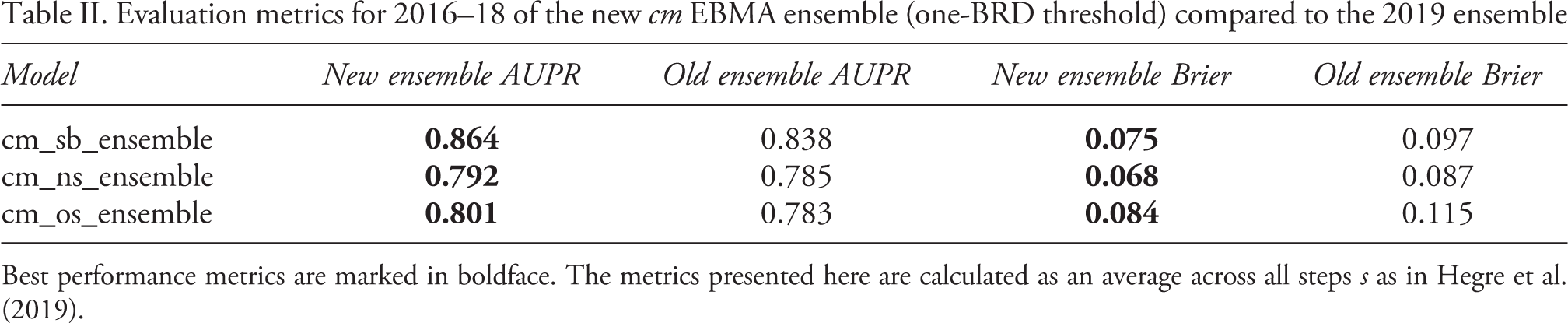
Best performance metrics are marked in boldface. The metrics presented here are calculated as an average across all steps s as in Hegre et al. (2019).

are more persistent and regular. Further, AUPR is generally lower when s is high, suggesting it is much more difficult to predict many months into the future. However, some models – especially those containing structural slow-moving features such as demography, political institutions, and economic indicators – improve predictive performance over time, at least relative to the conflict history models. For the ViEWS ambition to forecast over the full 36-month horizon, training models specifically for different s is clearly preferable. Finally, the main ensembles (ensemble_all) perform similar to or better than the best constituent model across outcomes and steps.

Online appendix D also shows the predictive performance of constituent models and ensembles for the pgm level. As expected given the difficulty of this prediction task, AUPR scores are markedly lower than for cm. As for cm, there are large differences in predictive performance between the constituent models, which largely mirror the divergence in relative performance that was seen in the cm analysis above.

Comparison with the 2019 model cm ensembles

We now turn our attention to the ensembles. In Online appendix D, we show that EBMA consistently outperforms unweighted ensembles for the sb outcome. To what extent are the new innovations improving forecasts? The results shown above are not directly comparable to Hegre et al. (2019), since we now require 25 battle-related deaths per month for violence to count as one of the conflict outcomes. To obtain comparable results, we ran a separate EBMA for the one battle-related death per month outcome using the constituent model predictions presented in Figure 3. The AUPR and Brier scores for ensemble_1brd and the old one are presented in Table II. The new ensemble is doing better across all outcomes and metrics.

Figure 4 shows the model criticism plot for the new sb ensemble. Compared to the old one (Figure 1), the new ensemble separates much better – the probability distribution for actual non-conflicts peaks at 0.02, and for

Figure 4.

Model criticism plot of current 1 BRD cm ensemble (test data: 2016–18)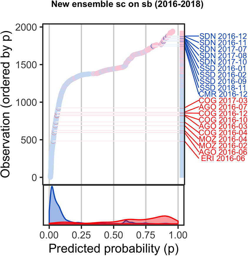

actual conflict at 0.90. In the prediction map in Figure 7 below, this is reflected as much larger variance in predicted probabilities than in Hegre et al. (2019). In Online appendix D, several biseparation plots show how the new ensemble ranks cases better than the old one.

Comparing previous published forecasts with actual events

ViEWS has produced updated forecasts every month since July 2018 based on the setup documented in Hegre et al. (2019). We use actual conflict data from two sources to evaluate the forecasting results: (i) UCDP-GED (Pettersson, Högbladh & Öberg, 2019) up to December 2018, and (ii) UCDP-Candidate (Hegre et al., 2020) thereafter.⁷

Figure 5.

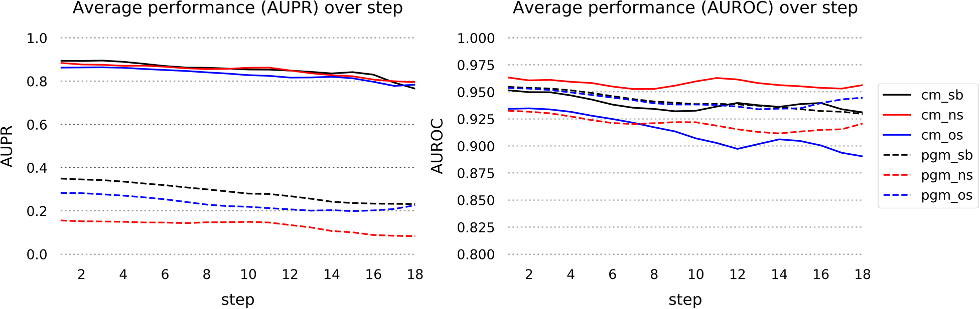
Areas under the Precision-Recall curve (AUPR, left), Area under the Receiver Operator Curve (AUROC, right), averaged across all runs with predictions, by s

Figure 6.

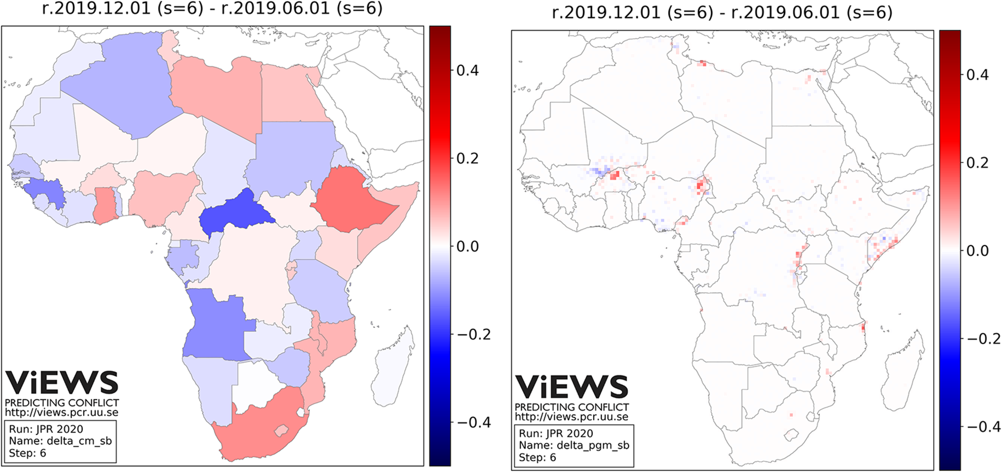
Changes in forecasted probability of sb conflict, $s = 6$ , June 2019–December 2019

Figure 5 shows the areas under the precision-recall curves (left) and the area under the receiver-operator curve (right) by steps s, for each outcome sb, os, ns, and each level of analysis.⁸ The figure shows that our forecasts are roughly as good as our out-of-sample evaluation indicated in Hegre et al. (2019, Figures 4, S-10, S-11), across all levels, outcomes, and steps.⁹

How have our forecasts changed over time?

Figure 6 shows how the ViEWS forecasts six months into the future changed from June 2019 to December 2019. The ensemble was unchanged over the period, so these changes are predominantly due to new observations of conflict events. Clusters of increased future probability of violence appear where fighting has recently escalated, such as in Tripoli, Cairo, Anglophone Cameroon, the Ituri province in DRC, and two provinces in

Figure 7.

ViEWS ensemble forecasts for 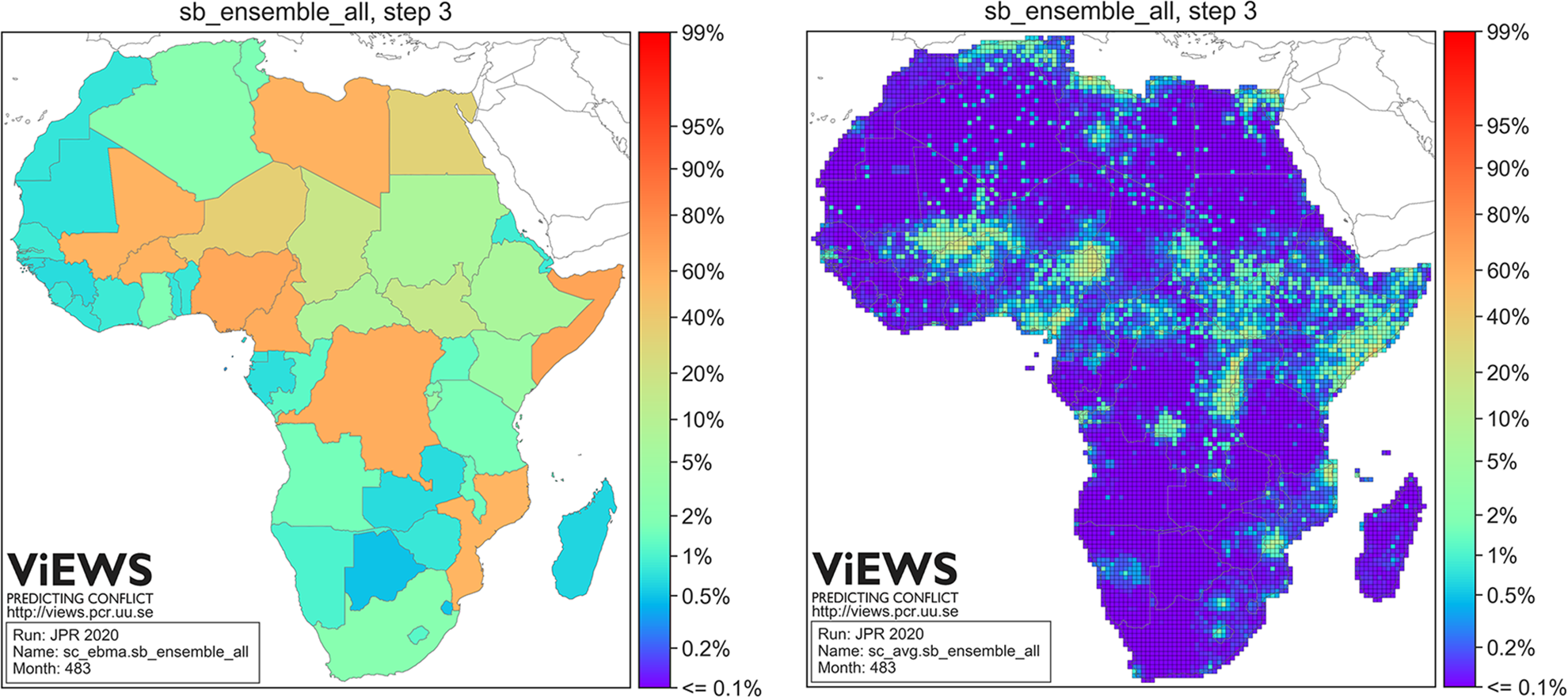sb, March 2020

Mozambique. While central Mali looks to be at lower risk of a state-based conflict event compared to June 2019, the risk has visibly increased for northern Burkina Faso.¹⁰ Moreover, regions that have been subject to protracted violence, such as southern Somalia’s coastal towns (including Mogadishu) and north-eastern Nigeria, show an escalated risk of state-based violence at

s = 6

, as compared to the June 2019 predictions.

Forecasts January 2020–December 2022

Figure 7 shows the predicted risk of state-based conflict in March 2020, at the cm (left) and pgm (right) levels, based on data up to and including December 2019. Figure 8 shows the trends in predicted probabilities over the entire forecasting period.

As we noted in Hegre et al. (2019), the expected conflict pattern in Africa remains remarkably stable. Nigeria, DRC, and Somalia are expected to remain the most conflict-prone countries in Africa, as our model predicts at least 25 BRDs in eight to nine out of 12 months during each of the coming three years. The pgm model suggests sb violence will be concentrated in the regions where violence has been most intense over the past few years, although there is a high risk of diffusion to central Nigeria and Puntland.

Cameroon, Burkina Faso, and Mozambique have a high predicted probability of conflict over most of 2020, but the model suggests the likelihood of violence is decreasing. Egypt and Sudan, on the other hand, are forecasted to increase conflict risk over the coming years.

To gain some intuition of what drives these forecasts, it is instructive to look at the predictions from individual models in the ensemble. Online appendix B shows the prediction maps for all cm models for various steps s. Given its recent conflict history, the thematic conflict history models cflong and acled_violence indicate a high probability of conflict in countries with recent violence, such as Nigeria, Burkina Faso, and Mozambique. However, also structural models such as vdem_glob, reign_glob, and wdi_all_glob contribute to the forecasts.

Figure 9 illustrates the contribution of each constituent model to the ensemble prediction for some example cases and various months.¹¹ Although the plots must be interpreted with caution, they can give a useful indication of what drives violence probability.¹² Important contributions to the ensemble come from conflict history

Figure 8.

Trends in predicted probabilities, cm level, ensemble, selected countries, January 2020–December 2022

Figure 9.

Contributions from constituent models to ensemble predictions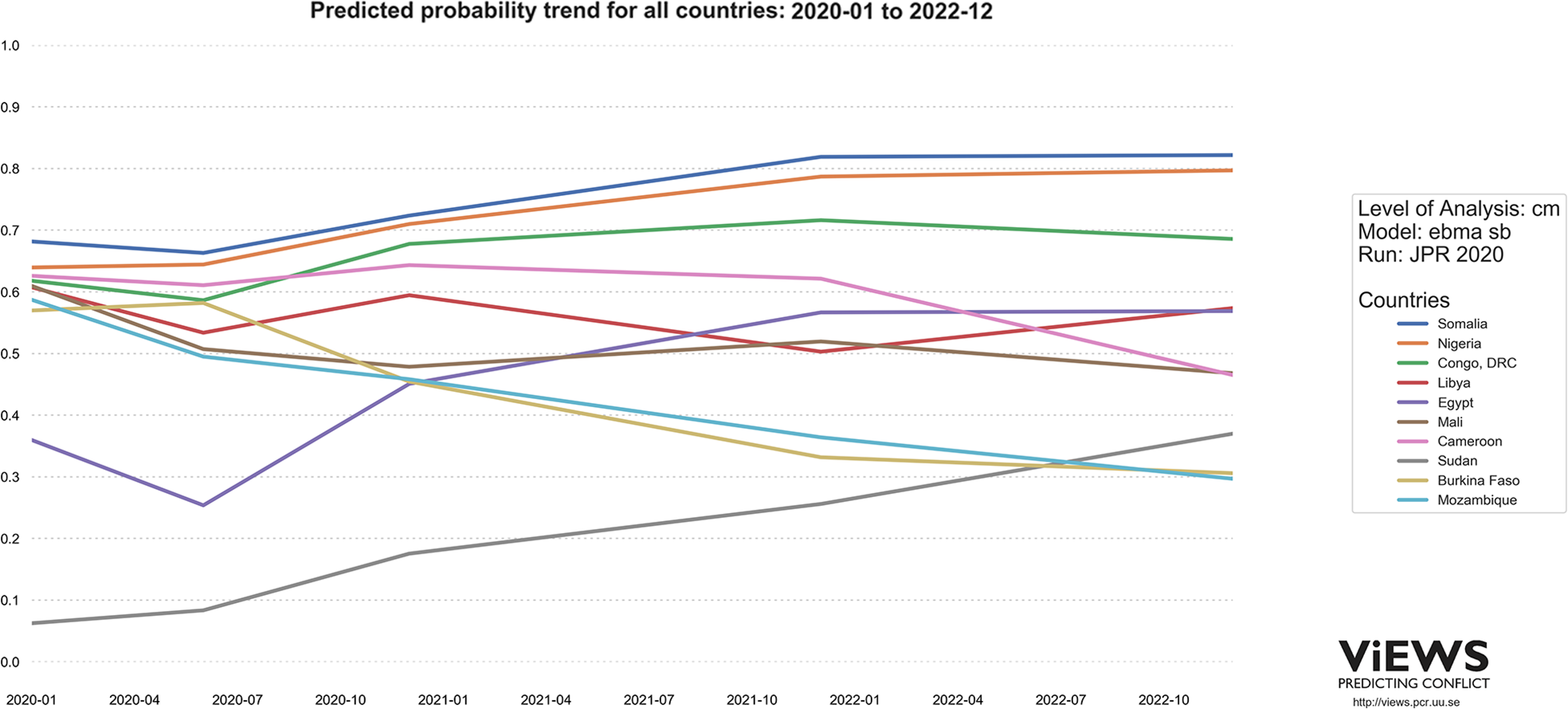

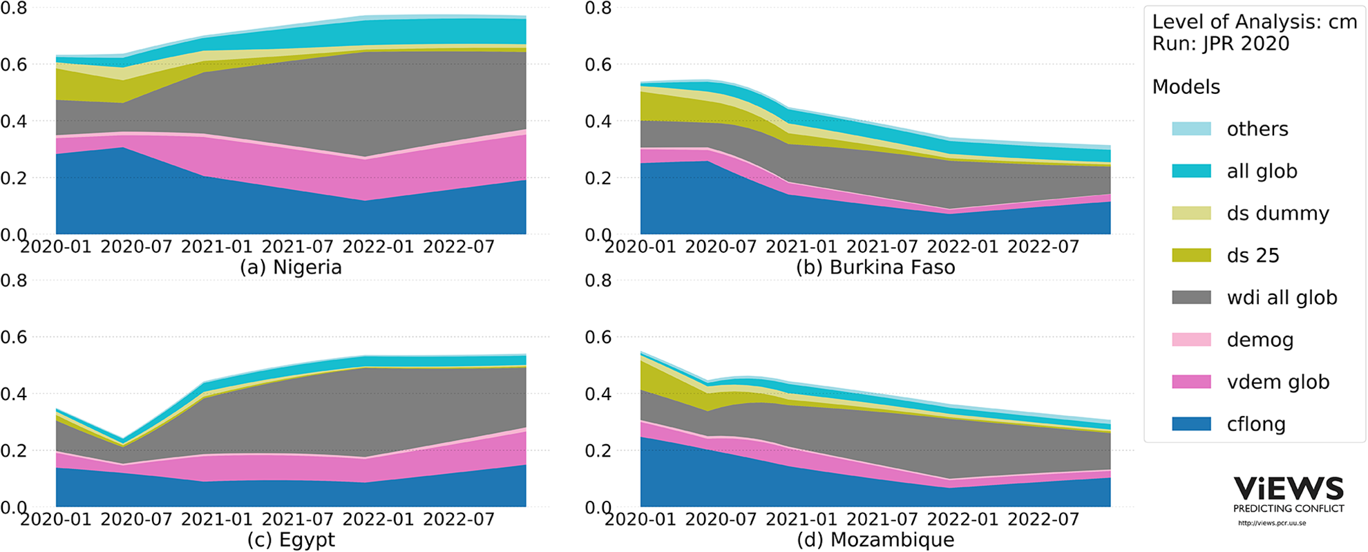
models (these are collected at the bottom of the stacks), of which cflong (blue) is the most important. Other main contributors are structural models (middle of the stack) such as vdem_glob (darker pink) and wdi_all_glob (gray). This is in line with what we find in terms of evaluation and predictive performance of broader compared to thematic models.

Figure 9a shows the risk profile for Nigeria. Much of the forecast is driven by conflict history, but as the forecasting horizon is extended, socio-economic and institutional factors become more important. The increasing probability in Egypt (9c) is mostly driven by socio-economic factors. The predicted decline in conflict probability in Burkina Faso (9b) relative to Nigeria is partly due to less high-risk political institutions, whereas the decline in Mozambique (9d) is attributed to a less intense conflict history.

Conclusion

The recent innovations in ViEWS summarized here improve the pilot and provide guidance for other conflict forecasting efforts. The new infrastructure for evaluating and weighting models makes better use of available data. This facilitates breaking the forecasting problem up into smaller pieces, which again helps us achieve some important objectives: it allows us to train and weight different models for the immediate and far-ahead future, and, for each time horizon, models representing different theoretical and methodological approaches to conflict forecasting. The current structure of constituent models that together form ensembles helps interpretability and allows for incremental improvement of the system.

We have shown that the new framework has improved overall performance, in particular with respect to effectively separating between high- and low-risk cases. New ‘structural’ models perform well with respect to new conflicts at the cm level, in particular for one to three years into the future. We have also documented the accuracy of the forecasts we have published every month based on Hegre et al. (2019), and demonstrated that the out-of-sample evaluation we conduct gives a precise indication of expected performance.

The new framework also opens up several avenues for future development. Ensembles of models are most effective and interpretable when constituent models are distinct from each other, while still performing well on their own. We will explore how to reduce correlation between models while retaining predictive performance. How to handle the distinctiveness/performance trade-off is an intriguing research question for which the conflict forecasting literature provides little guidance. For instance, broad models with large sets of features are important due to their ability to pick up interactive relationships between variables. However, they are obviously correlated with more distinct models that focus on a more narrow set of variables. Given the correlation, including both types of models means that the weight-based interpretation shown in Figure 9 becomes less useful. The optimal solution may be to identify breakdowns into smaller components of broad models (such as those based on WDI and V-Dem) that jointly maximize distinctiveness and overall performance.

Conversely, several constituent models such as protest and climate models are highly interesting from a substantial point of view. However, their poor performance tends to render them irrelevant or risk dragging down the performance of the ensemble. More work is required to specify such models carefully so that they better represent the underlying conflict dynamics associated with protest or climate change impacts, to tune them to maximize predictive performance for the relevant subset of conflict events.

Both of these model development approaches suggest we should strive to specify models that represent insights identified in the general conflict research literature published in this journal and elsewhere. We believe this is largely consistent with maximizing predictive performance, obviously a key criterion when developing a prediction ensemble. At the same time, this approach helps in understanding why armed conflict occurs, and how it can be prevented.

Footnotes

Replication data

Replication data and datasets with detailed predictions are available at https://views.pcr.uu.se/download/datasets/views_replication_jpr2020.zip, along with six Online appendices detailing our infrastructure (A), models at the cm (B) and pgm (C) levels, evaluation (D), our published forecasts (E), and the new predictions (F). Full source code is available at . All analyses were conducted using scikit-learn and R.

Acknowledgements

The authors would like to thank the editor and the anonymous reviewers for very helpful input, and Maikel Komen, Bruno Della Sala, Naa Adukwei Allotey, Micaela Wannefors, and Liana Lopes for assistance. For more information on the project, see .

Funding

ViEWS receives funding from the European Research Council (ERC) under the European Union’s Horizon 2020 research and innovation programme (grant agreement no. 694640) as well as from Uppsala University. Computations are performed on resources provided by the Swedish National Infrastructure for Computing (SNIC) at Uppsala Multidisciplinary Center for Advanced Computational Science (UPPMAX).

ORCID iD

Håvard Hegre

Mihai Croicu

Remco Jansen

Maxine Ria Leis

Angelica Lindqvist-McGowan

David Randahl

Paola Vesco

Notes

References

Armstrong

J Scott

(2001) Combining forecasts. In: Scott Armstrong

(ed.) Principles of Forecasting. New York: Springer, 417–439.

Belkin

Aaron

Schofer

Evan

(2003) Toward a structural understanding of coup risk. Journal of Conflict Resolution 47(5): 594–620.

Bell

Curtis

(2016) The Rulers, Elections, and Irregular Governance Dataset (REIGN) . Broomfield, CO: OEF Research (oefresearch.org).

Birch

Sarah

Daxecker

Ursula

Höglund

Kristine

(2020) Electoral violence: An introduction. Journal of Peace Research 57(1): 3–14.

Breiman

Leo

(2001) Random forests. Machine Learning 45(1): 5–32.

Cederman

Lars-Erik

Hug

Simon

Krebs

Lutz F

(2010) Democratization and civil war: Empirical evidence. Journal of Peace Research 47(4): 377–394.

Chen

Tianqi

Guestrin

Carlos

(2016) Xgboost: A scalable tree boosting system. Proceedings of the 22nd ACM SIGKDD International Conference on Knowledge Discovery and Data Mining, 785–794.

Colaresi

Michael

Mahmood

Zuhaib

(2017) Do the robot: Lessons from machine learning to improve conflict forecasting. Journal of Peace Research 54(2): 193–214.

Coppedge

Michael

Gerring

John

Lindberg

Staffan I

Skaaning

Svend-Erik

Teorell

Jan

Altman

David

Bernhard

Michael

Fish

Steven M

Glynn

Adam

Hicken

Allen

Knutsen

Carl Henrik

Krusell

Joshua

Lührmann

Anna

Marquardt

Kyle L

McMann

Kelly

Mechkova

Valeriya

Olin

Moa

Paxton

Pamela

Pemstein

Daniel

Pernes

Josefine

Petrarca

Constanza Sanhueza

Römer

Johannes von

Saxer

Laura

Seim

Brigitte

Sigman

Rachel

Staton

Jeffrey

Stepanova

Natalia

Wilson

Steven

(2017) V-Dem Country-Year Dataset v7.1. Varieties of Democracy (V-Dem) Project.

10.

Gleditsch

Kristian Skrede

(2002) All International Politics is Local: The Diffusion of Conflict, Integration, and Democratization. Ann Arbor, MI: University of Michigan Press.

11.

Greenhill

Brian

Ward

Michael D

Sacks

Audrey

(2011) The separation plot: A new visual method for evaluating the fit of binary models. American Journal of Political Science 55(4): 990–1002.

12.

Hegre

Håvard

(2018) Civil conflict and development. In: Walle

Nicholas van de

Lancaster

Carol

(eds) Oxford Handbook on the Politics of Development. Oxford: Oxford University Press, 177–199.

13.

Hegre

Håvard

Allansson

Marie

Basedau

Matthias

Colaresi

Mike

Croicu

Mihai

Fjelde

Hanne

Hoyles

Frederick

Hultman

Lisa

Högbladh

Stina

Jansen

Remco

Mouhleb

Naima

Muhammad

Sayeed Auwn

Nilsson

Desirée

Nygård

Håvard Mokleiv

Olafsdottir

Gudlaug

Petrova

Kristina

Randahl

David

Rød

Espen Geelmuyden

Schneider

Gerald

Uexkull

Nina von

Vestby

Jonas

(2019) ViEWS: A political Violence Early Warning System. Journal of Peace Research 56(2): 155–174.

14.

Hegre

Håvard

Croicu

Mihai

Eck

Kristine

Högbladh

Stina

(2020) Introducing the UCDP Candidate Events Dataset. Research and Politics 7(3). Available at: https://doi.org/10.1177/2053168020935257.

15.

Hegre

Håvard

Ellingsen

Tanja

Gates

Scott

Gleditsch

Nils Petter

(2001) Toward a democratic civil peace? Democracy, political change, and civil war, 1816–1992. American Political Science Review 95(1): 33–48.

16.

Montgomery

Jacob M

Hollenbach

Florian M

Ward

Michael D

(2012) Improving predictions using ensemble Bayesian model averaging. Political Analysis 20(3): 271–291.

17.

Pedregosa

Varoquaux

Gramfort

Michel

Thirion

Grisel

Blondel

Prettenhofer

Weiss

Dubourg

Vanderplas

Passos

Cournapeau

Brucher

Perrot

Duchesnay

(2011) Scikit-learn: Machine learning in Python. Journal of Machine Learning Research 12: 2825–2830.

18.

Pettersson

Therése

Högbladh

Stina

Öberg

Magnus

(2019) Organized violence, 1989–2018 and peace agreements. Journal of Peace Research 56(4): 589–603.

19.

Raleigh

Clionadh

Hegre

Håvard

Karlsen

Joakim

Linke

Andrew

(2010) Introducing ACLED: An Armed Conflict Location and Event Dataset. Journal of Peace Research 47(5): 651–660.

20.

Russell

Stuart J

Norvig

Peter

(2016) Artificial Intelligence: A Modern Approach. London: Pearson Education.

21.

Tollefsen

Andreas Forø

Strand

Håvard

Buhaug

Halvard

(2012) PRIO-GRID: A unified spatial data structure. Journal of Peace Research 49(2): 363–374.

22.

Vicente-Serrano

Sergio M

Beguería

Santiago

López-Moreno

Juan I

(2010) A multiscalar drought index sensitive to global warming: The Standardized Precipitation Evapotranspiration Index. Journal of Climate 23(7): 1696–1718.

23.

von Uexkull

Nina

Croicu

Mihai

Fjelde

Hanne

Buhaug

Halvard

(2016) Civil conflict sensitivity to growing-season drought. Proceedings of the National Academy of Sciences 113(44): 12391–12396.

24.

World Bank (2019) World Development Indicators. Washington DC: World Bank.

ViEWS 2020 : Revising and evaluating the ViEWS political Violence Early-Warning System

Abstract

Keywords

Overview

Revising the ViEWS pilot

Changes to how we handle data for model evaluation and averaging

Changes to dependent variables

Ensembles

New set of constituent models

New models and data at cm level

New models at pgm level

Evaluation

Constituent models

Comparison with the 2019 model cm ensembles

Comparing previous published forecasts with actual events

How have our forecasts changed over time?

Forecasts January 2020–December 2022

Conclusion

Footnotes

Replication data

Acknowledgements

Funding

ORCID iD

Notes

References