ViEWS: A political violence early-warning system

Abstract

This article presents ViEWS – a political violence early-warning system that seeks to be maximally transparent, publicly available, and have uniform coverage, and sketches the methodological innovations required to achieve these objectives. ViEWS produces monthly forecasts at the country and subnational level for 36 months into the future and all three UCDP types of organized violence: state-based conflict, non-state conflict, and one-sided violence in Africa. The article presents the methodology and data behind these forecasts, evaluates their predictive performance, provides selected forecasts for October 2018 through October 2021, and indicates future extensions. ViEWS is built as an ensemble of constituent models designed to optimize its predictions. Each of these represents a theme that the conflict research literature suggests is relevant, or implements a specific statistical/machine-learning approach. Current forecasts indicate a persistence of conflict in regions in Africa with a recent history of political violence but also alert to new conflicts such as in Southern Cameroon and Northern Mozambique. The subsequent evaluation additionally shows that ViEWS is able to accurately capture the long-term behavior of established political violence, as well as diffusion processes such as the spread of violence in Cameroon. The performance demonstrated here indicates that ViEWS can be a useful complement to non-public conflict-warning systems, and also serves as a reference against which future improvements can be evaluated.

Keywords

Africa armed conflict forecasting

ViEWS: Guiding principles

Large-scale political violence kills thousands every month across the globe and forces many more to relocate within countries and across borders. Armed conflicts have disastrous economic consequences, undermine the functioning of political systems, prevent countries from escaping dire poverty, and hinder humanitarian assistance where most needed.

The challenges of preventing, mitigating, and adapting to large-scale political violence are particularly daunting when it escalates in locations and at times where it is not expected. Policymakers and first responders would benefit greatly from a system that systematically monitors all locations at risk of conflict and assesses the probability of conflict onset, escalation, continuation, and geographic diffusion. This article presents ViEWS – a political violence early-warning system — which seeks to address this need. We outline the methodological framework and evaluate the predictive performance of the system as of 1 October 2018.

The forecasting task ViEWS has set out is multidimensional. ViEWS provides forecasts 36 months into the future for three types of political violence: armed conflict involving states and rebel groups, armed conflict between non-state actors, and violence against civilians (Pettersson & Eck, 2018). The probability that political violence occurs in a given month is forecasted for both countries and subnational geographical units. This means that ViEWS provides forecasts for continued conflict as well as new conflicts. To be useful as an early-warning system, ViEWS has since June 2018 published monthly updated forecasts for Africa at http://views.pcr.uu.se/.¹ This is made possible by the monthly release of candidate events from the Uppsala Conflict Data Program (UCDP; see Hegre et al., 2018).

The ViEWS forecasts build on a number of constituent models drawing on insights from decades of quantitative peace and conflict research. Some of the models are thematic, concentrating on topics such as conflict history, the economy, political institutions, and geography. Others are more general, combining multiple themes or using information at the country and the subnational level to generate forecasts. We subsequently combine the forecasts from these individual models to ensembles. Our evaluation shows that the ViEWS ensembles improve forecasting of political violence at both the country and the subnational level compared to multiple tough baseline models.

The forecasts from October 2018 indicate that conflict will persist up to and beyond 2021 in several countries that have a recent history of political violence, such as Burundi, Nigeria, and DR Congo. The system also alerts to new conflicts in Southern Cameroon and Northern Mozambique.

The aims of ViEWS are maximal transparency, uniform coverage, and public availability. Transparency requires that the risk assessments can be traced back to a fully specified argument and accessible information, allowing readers and potential users to evaluate what lies behind the forecasts. ViEWS is therefore exclusively based on publicly available data. Moreover, its results, input data, and procedures are available to researchers and the international community. Uniform coverage of the regions at risk helps to alert observers to locations that receive insufficient attention. In principle, ViEWS seeks to be able to issue a warning with equal probability for any location independent of its geo-strategic importance, past conflict history, or current humanitarian situation. Public availability of the results is useful for domestic actors and small international NGOs, and essential to ensure transparency regarding decisions they might make based on these results.

In the following, we first briefly review the literature that has informed ViEWS. Second, we outline the methodological framework. Third, we evaluate the performance of the system and present the ViEWS forecasts from October 2018 to October 2021. Finally, we discuss future extensions of the system and conclude.

Literature review

Prediction has long been considered a core task for peace research (Singer, 1973), and a comprehensive literature review is beyond the scope of this article (rather, see Schneider, Gleditsch & Carey, 2010; Hegre et al., 2017). Conflict forecasting has taken a number of methodological approaches, for example game theory (Bueno de Mesquita, 2010), machine-learning tools such as neural networks (Schrodt, 1991), and algorithms for automatic coding of event data (Schrodt, Davis & Weddle, 1994). Ward, Greenhill & Bakke (2010) arguably represents a turning point, bringing prediction into the mainstream of peace research.

ViEWS builds on innovations in the academic early-warning systems for conflict that have been proposed since the 1970s (Andriole & Young, 1977). The State Failure/Political Instability Task Force (PITF) aimed to forecast political crises two years in advance (Esty et al., 1995; Gurr et al., 1999; Goldstone et al., 2010). A key insight from PITF is that simplistic models with a few powerful variables performed as well as complex models, at least at the country-year level. The Integrated Crisis Early Warning System (ICEWS) focused on a range of domestic and international crises (O’Brien, 2010). Valuable insights from ICEWS include separate modelling of conflict phases (onset, continuation, termination) and the utility of a multimethod approach to forecasting.

As the literature has matured, real-time forecasts have become increasingly common (Brandt, Freeman & Schrodt, 2011; Ward & Beger, 2017). Some of these are publicly available. For instance, the US Holocaust Memorial Museum has a regular updated early-warning system for mass atrocities (https://www.ushmm.org/confront-genocide/how-to-prevent-genocide/early-warning-project), and One Earth Future publishes monthly forecasts for military coups (CoupCast; http://oefresearch.org/activities/coup-cast).

Some contributions have been particularly important for ViEWS. We build on the pioneering work of Michael Ward and his team (Montgomery, Hollenbach & Ward, 2012; Ward & Beger, 2017) using ensemble methods to combine forecasts from unique thematic models. We also adapt efforts to integrate structural factors with temporally and spatially disaggregated event data that change more swiftly (Weidmann & Ward, 2010; Chiba & Gleditsch, 2017). Our evaluation builds on the introduction of ROC curves to peace research (Ward, Greenhill & Bakke, 2010), PR curves (O’Brien, 2002), Brier scores (Brandt, Schrodt & Freeman, 2014), and separation plots (Greenhill, Ward & Sacks, 2011; Colaresi & Mahmood, 2017). We also use the random forest algorithm (Breiman, 2001) which has been shown to be effective in our domain (Colaresi & Mahmood, 2017).

Finally, ViEWS would not have been possible without the extensive substantive research on armed conflict (see Buhaug, Levy & Urdal, 2014; Gleditsch, Metternich & Ruggeri, 2014; Hegre & Sambanis, 2006, for reviews). ViEWS has greatly benefited from civil war studies conducted at the country level (e.g. Muller & Weede, 1990; Fearon & Laitin, 2003), but also from the geographically disaggregated studies initiated in the early 2000s (Buhaug & Gates, 2002; Buhaug, Cederman & Red, 2008; Cederman & Gleditsch, 2009), made possible by the geo-coded events data (Raleigh et al., 2010; Sundberg & Melander, 2013).

Methodology

To address its forecasting task, ViEWS is organized into smaller subtasks following a ‘divide and conquer’ strategy detailed in this section. We describe how we analyze three outcomes separately at two levels of analysis, and eventually combine all models using ensembles to produce the ViEWS forecast. The workflow for each monthly update is sketched in Figure 1. All steps in this process are automatized as a set of SQL and Python 3.x scripts. Data are handled on a dedicated server, whereas most model training and simulation is run on a high-performance computing cluster. Further methodological details and additional results are in an Online appendix, the sections of which are referred to as ‘Appendix [no.]’.

Levels of analysis

ViEWS generates forecasts at two levels of analysis: country-months (Gleditsch & Ward, 1999, abbreviated cm), and subnational geographical location months (pgm). The cm level is useful for predictions of new conflicts where no known actors exist, and to model processes at the government level. The set of countries is defined as in Gleditsch & Ward (1999), and the geographical extent of countries by CShapes (Weidmann, Kuse & Gleditsch, 2010). For the subnational forecasts, ViEWS relies on the PRIO-GRID (version 2.0; Tollefsen, Strand & Buhaug, 2012), a standardized structure consisting of quadratic grid cells that cover all areas of the world at a resolution of 0.5 x 0.5 decimal degrees. More details on the levels of analysis are in Appendix B.1.

The outcomes we predict: Conflict data

ViEWS generates predictions for the three forms of organized violence coded by the UCDP (Melander, Pettersson & Themnér, 2016): state-based conflict (sb), one-sided violence against civilians (os), and non-state conflict (ns).² We are convinced that an early-warning system benefits from distinguishing between these forms of violence. They are related, but also distinct: democracies see less armed conflict (Hegre et al., 2001), but rebel groups fighting democratic governments are more likely to target civilians than those fighting autocrats (Eck & Hultman, 2007). Non-state conflicts are much more responsive to climatic factors than state-based conflicts (Fjelde & von Uexkull, 2012). As ViEWS improves its thematic models, these distinctions are important to maintain.

We focus primarily on state-based conflicts here to simplify presentation. sb conflicts are more numerous than os and ns, and have been studied more extensively. A large share of os and ns events are also outcomes of state-based conflicts: much of the violence against civilians is perpetrated by governments and rebel groups to weaken opponents, and much non-state conflict is in-fighting between rebel groups that also are in conflict with the government.

Conflict data are obtained from UCDP-GED and take the form of events (Sundberg & Melander, 2013). Historical data covering 1989–2017 are extracted from the UCDP GED version 18.1 (Croicu & Sundberg, 2013; Allansson, Melander & Themnér, 2017;

Figure 1.

The ViEWS system and monthly process flow in six steps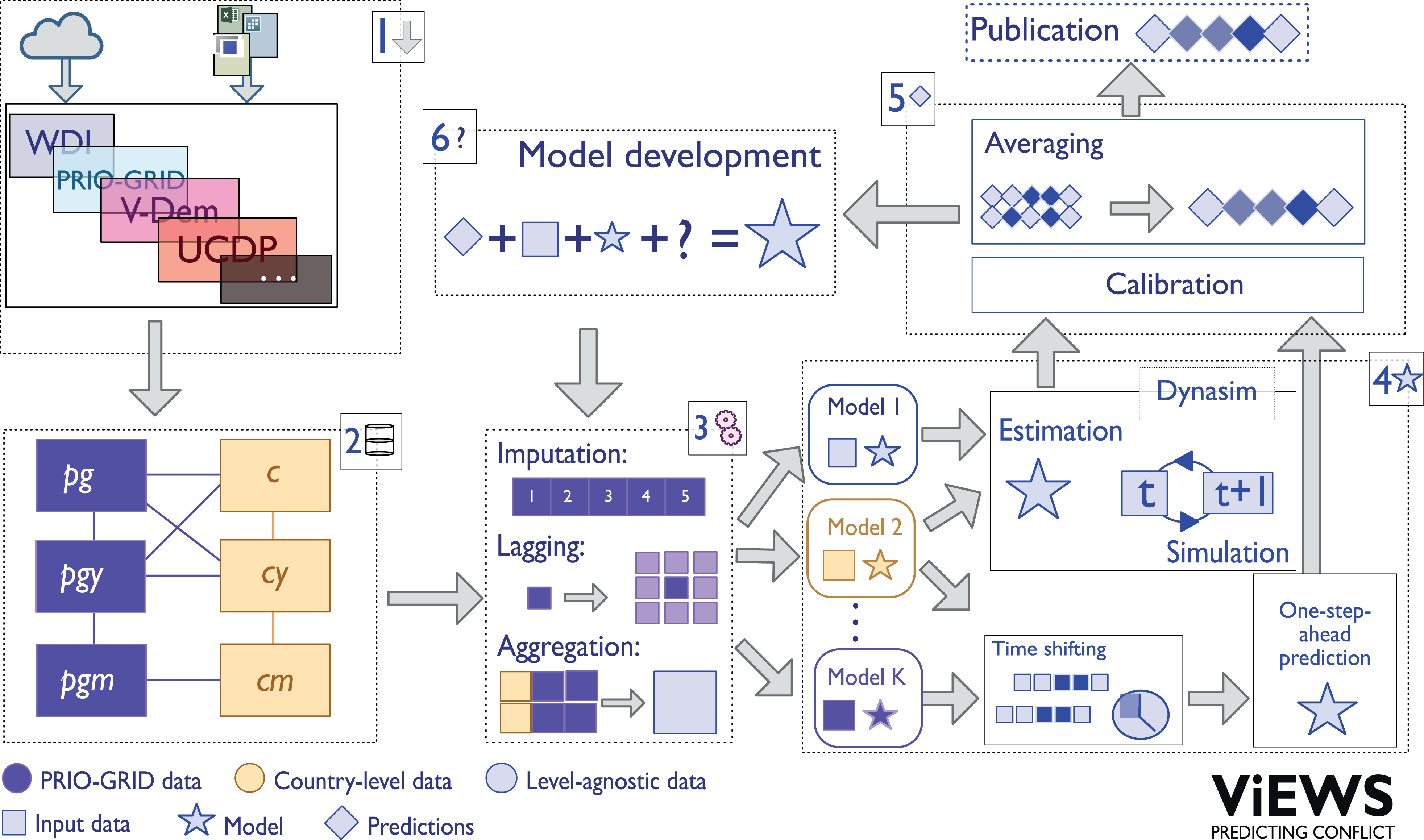

Pettersson & Eck, 2018).³ Newer data are provided by the new UCDP-Candidate dataset which is updated monthly (see Hegre et al., 2018, and Appendix B.2 for details regarding definitions and aggregation). These updates enable using data on conflict up to one month before the forecasting window. Here, we use data including August 2018. The UCDP-Candidate data are in the form of ‘candidate events’. Many UCDP definitions (see Gleditsch et al., 2002) are applicable only on a per calendar-year basis, and the final UCDP-GED dataset can only be compiled after the end of the year. The UCDP-Candidate events dataset consequently relaxes the UCDP requirement of 25 battle-related deaths in a calendar year for a conflict to be recorded, as well as the requirement of a ‘stated goal of incompatibility’. The very strict requirements in terms of known and clear parties to the conflict are also relaxed as long as there are sufficiently strong indications that events have a high likelihood of inclusion in the final UCDP datasets. UCDP and ViEWS have developed a coding procedure with a goal of making the monthly candidate events as close in content to the final dataset as possible.

The statistical models constituting ViEWS

The models in ViEWS (summarized in Table I) are designed to complement each other. As of October 2018, ViEWS has specified two extensive and six thematic core models at the cm level. At the pgm level there are ten core models – five thematic, two combined themes, and three with country-level predictors. We use three different estimation strategies for each of these core models. We combine these models in ensembles to produce the ViEWS forecasts – 24 models in the cm ensembles, and 30 in pgm. We estimate the same ensembles of models for each of the three outcomes (sb, ns, and os).

Table II lists the models at the cm level. Detailed descriptions of the predictors can be found in Appendix A, and estimation results are available in Jansen et al. (2018). Figure 2 shows maps of the predicted probabilities for a subset of the models. These refer to at least one event in a country month for sb conflict, October 2018.

Table I.

Overview of models, and abbreviations, used in the ViEWS ensemble

Model group definition	Group	Notes
Levels of analysis	cm	Country-month level
Levels of analysis	pgm	PRIO-GRID-month level
Outcomes	sb	State-based conflict
	os	One-sided violence
	ns	Non-state conflict
Predictor aggregation	Thematic, no cross-level representation	6 themes at cm and 4 at pgm levels. See Tables II and III
	All themes, no cross-level representation	One variant with protests, one without pgm level only
	All themes and cross-level representation
Handling of dynamics and estimation strategy	Dynamic simulation	See section ‘Dynamic simulation’
	One-step ahead logit
	One-step ahead random forest

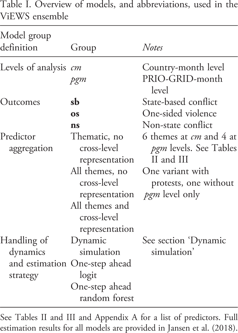
See Tables II and III and Appendix A for a list of predictors. Full estimation results for all models are provided in Jansen et al. (2018).

Countries with red color have predicted probabilities close to 1, whereas blue and purple countries have probabilities at less than 0.01. Orange means a predicted probability of 0.5.

The baseline model (not mapped) uses the average proportion of months with conflict in a country over the 1990–2014 period as a single predictor. The conflict history theme represents the more recent record of conflict events. As is shown in Figure 2a, the predictions for this model reflect recent violence in for instance Nigeria, DRC, and Mali. The demography, economy, institutional, and protest themes capture elements from the peace research literature. Figure 3 shows that the demography model yields somewhat heightened predicted probabilities for populous countries and countries with low education rates (Raleigh & Hegre, 2009; Thyne, 2006). The economics model (2c) suggests more conflict in poor or oil-producing countries with low economic growth (Collier, Hoeffler & Söderbom, 2004; Fearon & Laitin, 2003). The institutional model (2d) assigns high risk to countries that are non-democratic, exclude large minorities from political power, and with recent regime changes (Hegre et al., 2001; Cederman, Hug & Krebs, 2010;

Table II.

cm (country-level) models

Baseline

Proportion of months in training period with conflict

Conflict history theme

Lagged conflict (sb, ns, os)

Decay functions (

2^{- m / 12}

where m is the number of months without conflict and 12 months the half-life parameter; sb, ns, os)

Demography theme

Population size

Proportion of population between 15 and 24 with at least lower secondary education

Proportion of population living in urban areas

Economy theme

GDP per capita, oil rents only

GDP per capita, excluding oil rents

Growth in GDP per capita, oil rents only

Growth in GDP per capita, excluding oil rents

Institutions theme

Democracy

Semi-democracy

Time since pre-independence war

Time since regime change

Proportion of population excluded from power

Time since independence

Protest theme

Lagged protest

Decay functions (

2^{- m / 12}

where m is the number of months without protest and 12 months the half-life parameter)

All themes

Baseline + Conflict history +

Demography + Economy + Institutions

All themes + protest

Baseline + Conflict history +

Demography + Economy + Institutions + Protests

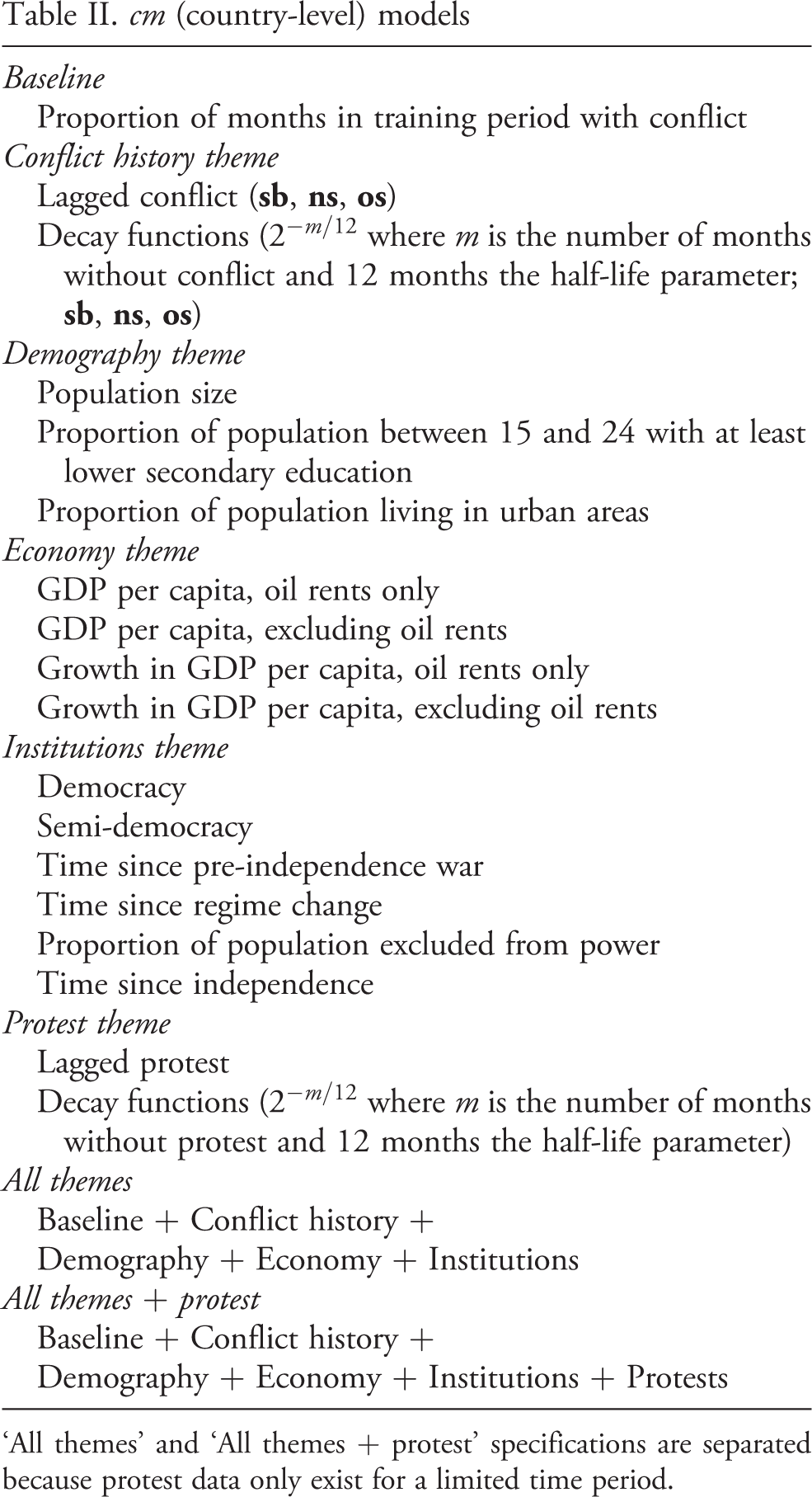
‘All themes’ and ‘All themes + protest’ specifications are separated because protest data only exist for a limited time period.

Cederman, Wimmer & Min, 2010). The protest model (2e) captures that protest can be a precursor to armed conflict, as it was in Syria in 2011 and Burundi in 2015. Escalation can be especially likely when the government responds with violence (Tilly, 1978). The map shows that the protest theme overall assigns relatively high probability of conflict throughout Africa, but lower in a handful of peaceful countries, among them Zambia and Botswana. However, the protest theme also assigns low probabilities to conflict-prone countries such as the Central African Republic and Chad. The final dimension of model variation relates to estimation strategy and handling of dynamics (cf. Table I and sections ‘Model estimation’ and ‘Handling forecasting dynamics’ below). Figure 2f shows predictions from the demography model

Figure 2.

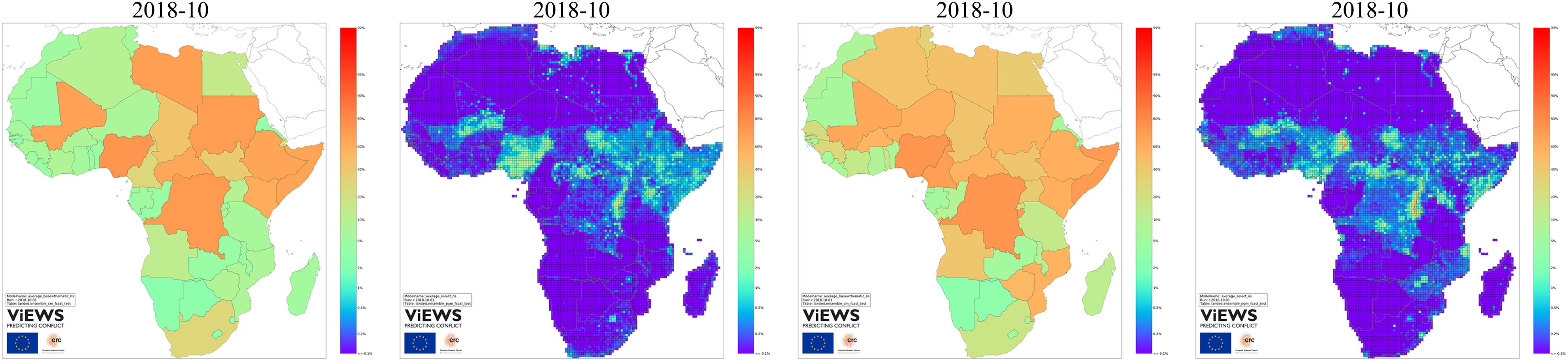
Country-level sb forecasts for October 2018, selected constituent models

produced when estimating a one-step-ahead random forest model. Comparing 2b and 2f we see a much stronger discrimination between high and low risk countries in 2f, even though the same predictors enter both models. For all models, the one-step-ahead random forests tend to give sharper predictions compared to dynamic simulation and one-step-ahead logits.

Table III summarizes the ViEWS models at the pgm level, and their prediction maps are shown in Figure 3. As for the cm level, the baseline uses the proportion of months with conflict for each PRIO-GRID cell as a predictor. The conflict history theme captures recent events in a cell and its neighbors. As shown in Figure 3a, conflict history yields specific and sharp predicted locations of conflict in October 2018.

We have defined two themes with relatively static geographical predictors, one for natural features and one for social ones. Figure 3b shows that the natural geography model indicates an elevated risk of conflict in areas that are attractive for human habitation, and areas such as those in Angola, Namibia, and Botswana that are close to diamond and oil extraction sites (Le Billon, 2001; Lujala, Gleditsch & Gilmore, 2005). The prediction from the social geography theme in 3c highlights the risk in highly populated or low-income areas, as well as locations with politically excluded ethnic groups, close to borders, or far from capitals (Raleigh & Hegre, 2009; Buhaug, Gates & Lujala, 2009; Wucherpfennig et al., 2011). Figure 3d shows the predictions from the protest theme. The theme assigns higher probabilities to countries such as Tunisia, Burundi, Rwanda, and a number of countries in Western Africa.

We have also specified a number of large models that include all the thematic predictors. Figure 3e shows the predictions from a model including history, natural geography, and social geography as well as cm level predictors. This large model pulls up the predicted probabilities for locations in countries that the cm models indicate are relatively high risk (e.g. Angola and Zimbabwe), and pulls down probabilities for countries like Namibia and Botswana.

Finally, Figure 3f shows a model containing the same predictors as 3e but modelled using one-step-ahead random forests instead of dynamic simulation. When

Figure 3.

PRIO-GRID level 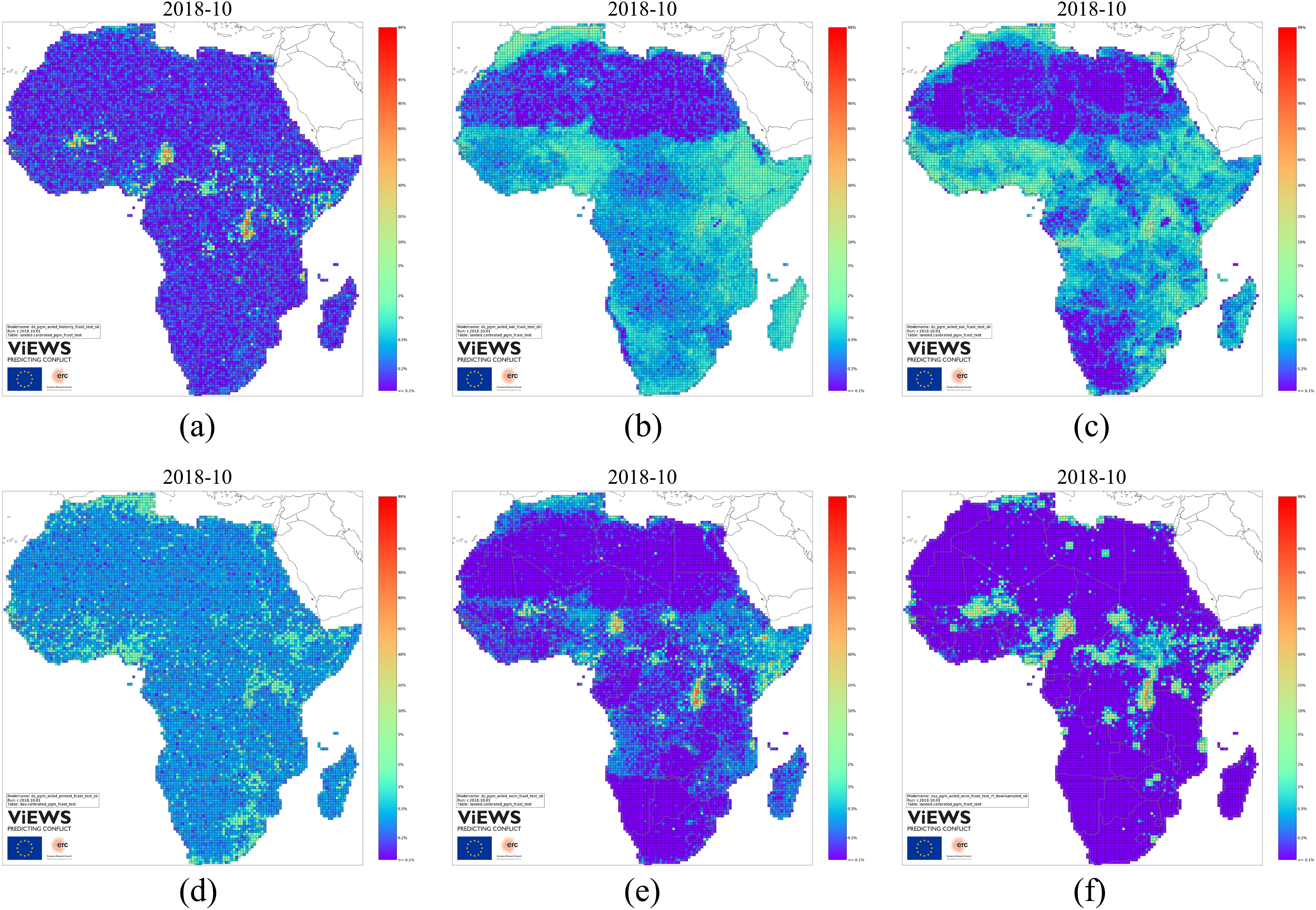sb forecasts for October 2018, selected constituent models

comparing 3e and 3f, we see that the random forest model provides smaller areas with high predicted probability of conflict than the dynamic simulation model.

Data sources for predictors

Complete references to the data sources are in Appendix A. The most important sources are PRIO-GRID (Tollefsen, Strand & Buhaug, 2012), the World Development Indicators (World Bank, 2015), data on politically excluded ethnic groups (Cederman, Wimmer & Min, 2010), demographic factors (Lutz et al., 2007), protests from ACLED (Raleigh et al., 2010), and data on institutions from V-Dem (Coppedge et al., 2011).

Model estimation

ViEWS relies on logistic regression and random forest models. The logit model is a generalized linear model (GLM) that performs well compared to many machine-learning techniques (Géron, 2017). The random forest model (Breiman, 2001; Muchlinski et al., 2016) is a machine-learning technique based on a combination of classification and regression trees (CART), bootstrap-aggregating (bagging), and random feature selection. Because random forest models are computationally intensive, we estimate them using a ‘downsampled’ dataset which includes all conflict events and a random sample of non-events. See Appendixes C.1 and D.1 for more details.

Handling forecasting dynamics

ViEWS employs two alternative strategies to compute forecasts for each of $s \in (1, .., 36)$ months into the future. We call these dynamic simulation (ds) and one-step-ahead (osa).

Dynamic simulation

The dynamic simulation (Dynasim) procedure builds on Hegre et al. (2013) and Hegre et al. (2016), and is discussed at length there.⁴ The

Table III.

pgm (PRIO-GRID level) models

Baseline

Proportion of months in training period with conflict

Conflict history theme

Lagged conflict event (sb, ns, os)

Months since last conflict (decay function

2^{- m / 12}

; sb, ns, os)

Spatial lag of lagged conflict event (sb, ns, os)

Natural geography theme

Distance to nearest secondary diamonds resource

Distance to nearest petroleum resource

Proportion of mountainous terrain

Agricultural area

Barren area

Forest area

Shrublands

Pasture land

Urban areas

Social geography theme

Distance to neighboring country

Travel time to nearest city

Distance to capital city

Population size

Gross cell product

Infant mortality rate

Number of excluded groups

Country-level (cm) theme

Democracy

Semi-democracy

Time since independence

Time since pre-independence war

Time since regime change

Proportion of population excluded

GDP per capita, oil rents only

GDP per capita, excluding oil rents

Growth in GDP per capita, oil rents only

Growth in GDP per capita, excluding oil rents

Population size

Proportion of population between 15 and 24 with at least lower secondary education

Proportion of population living in urban areas

Protest theme

Lagged protest

Months since last protest (decay function

2^{- m / 12}

)

Spatial lag of protest

All themes, without cm

Baseline + Conflict history +

Natural geography + Social geography

All themes, with cm

In this model, predictions are either generated by (1) adding the ‘cm theme’ variables to the ‘All themes, without cm’ model; or (2) multiplying predictions from the ‘All themes, without cm’ model predictions obtained from estimation at the pgm level with predictions from the ‘All themes’ model estimated at the cm level. For details on (2), see section on cross-level representation.

All themes, without cm + protest

Baseline + Conflict history +

Natural geography + Social geography + Protest

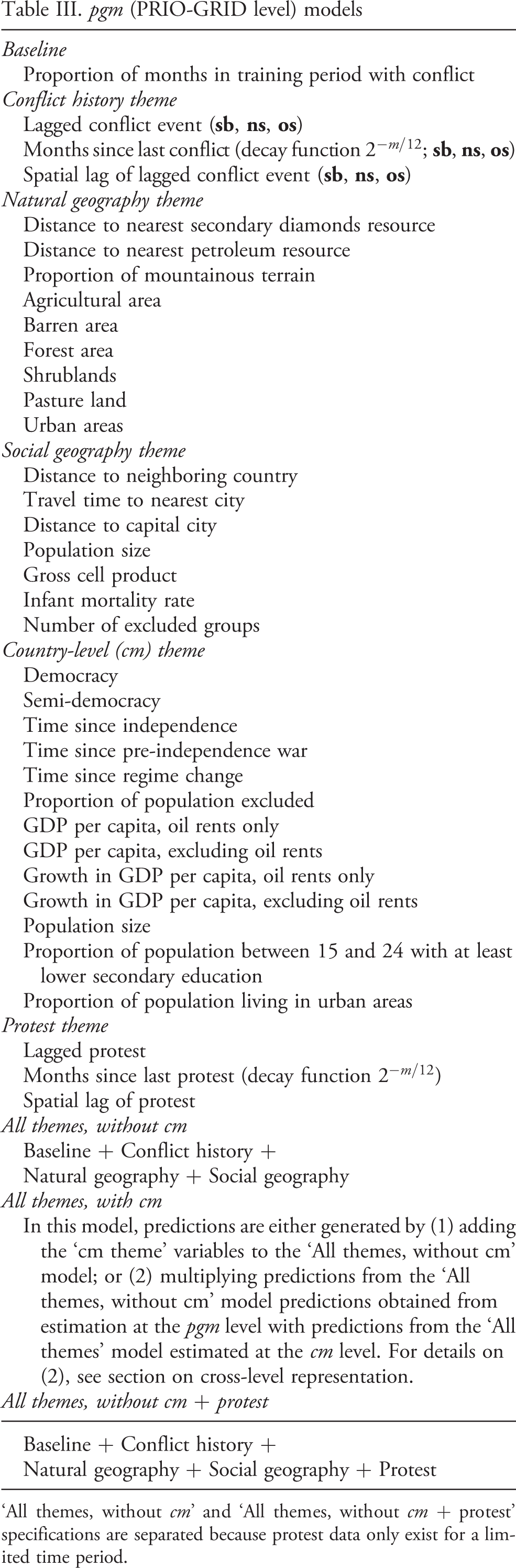
‘All themes, without cm’ and ‘All themes, without cm + protest’ specifications are separated because protest data only exist for a limited time period.

procedure involves simulating model parameters based on the estimated coefficients and the variance-covariance matrix from a model. In addition, we compute predicted probabilities for the outcomes for the first month t, draw outcomes, and recalculate the history variables so that the input predictor matrix

X_{t + 1}

at t + 1 reflects that draw. This is repeated for each month s in the forecasting window, and for each simulated set of parameters.

If we are interested in forecasting two months into the forecasting period, we first train the constituent models, estimate the weights, and produce our ensemble one-month-ahead forecast. To produce forecasts for the next month, we need the input predictor matrices $X_{t + 1}^{(k)} .$ For many constituent models, these input predictors will themselves be functions of actual conflict (e.g. lagged conflict indicators, time since last conflict, spatial distance to nearest conflict). Since these do not exist for the next month (after the training window), we use the prediction as the probability of an unobserved predictor, for example for conflict at time t + 1, when forecasting conflict at t + 2. A simulated value is drawn from this probability, and recorded within a new simulated set of predictors ${\tilde{X}}_{t + 1}^{(k)}$ .

The predictions for the three outcomes are obtained simultaneously within each time step. For each of these, we compute the predicted probability at t + 1 as a function of information available at t, including the status for the other two outcomes. This procedure repeats for every month to the end of the forecasting window.

‘One-step-ahead’ modeling

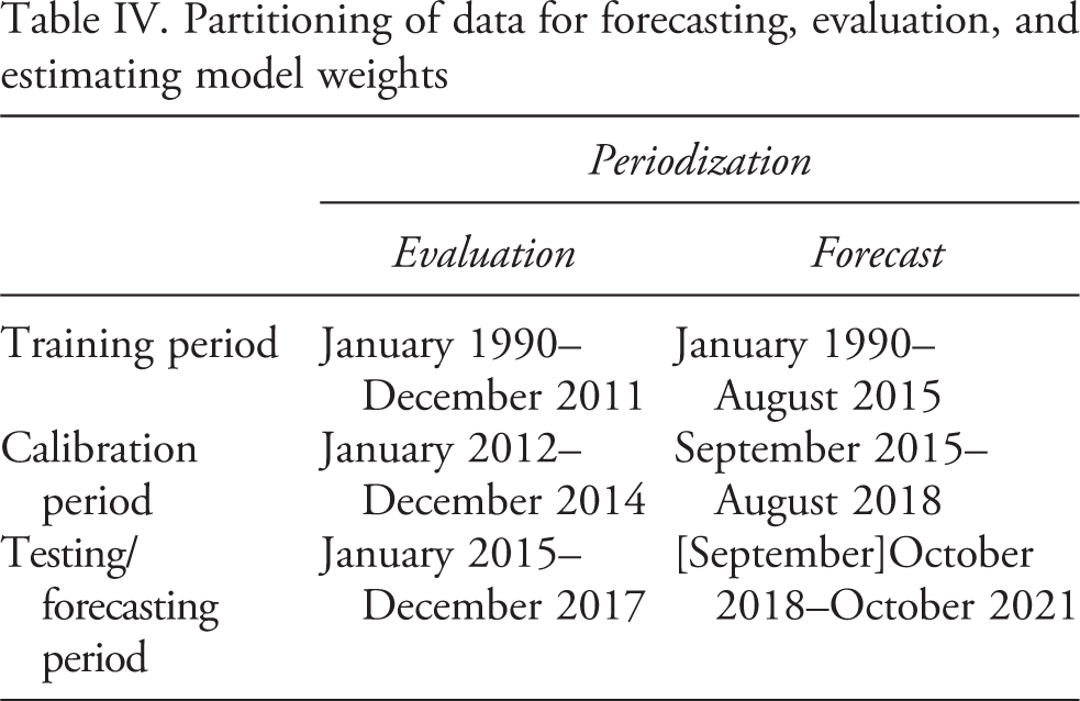
In the one-step-ahead modeling, we predict each step into the future (t + 1, (…), t + 12, (…) t + 36) independently, as opposed to dynamic simulation which moves forward sequentially. We do this by estimating a set of models of the form $f_{s} (X_{t - s})$ where s denotes the number of months into the future to forecast. In regression notation these take the form $y_{t + s} = X_{t} β_{t}, f o r s \in (1, 36)$ . The one-step-ahead mode does this by time-shifting the right-hand side variables with respect to the outcome before models are trained, making the model a link function between the future ( $y_{t + s}$ ) and the present ( $X_{t}$ ).

Table IV.

Partitioning of data for forecasting, evaluation, and estimating model weights

	Periodization
	Evaluation	Forecast
Training period	January 1990– December 2011	January 1990– August 2015
Calibration period	January 2012– December 2014	September 2015– August 2018
Testing/forecasting period	January 2015– December 2017	[September]October 2018–October 2021

Data partitioning and calibration

Table IV summarizes how we partition the data in ViEWS. When evaluating our models, we need a held-out test set for which we have observed conflict. We call this the ‘evaluation periodization’. We use the three most recent years for which we have final UCDP-GED data as the test period – currently, 2015–17. When forecasting, the future is the test set. In this case, we use all of our available data to train and calibrate the forecasting models. We call this the ‘forecasting periodization’.⁵ For each of these two periodizations, we partition our data into three periods: one for estimating or training statistical models, one for calibrating predicted probabilities from the models, and one for testing and forecasting.

All our models are initially estimated on the training period. Based on this estimation, we generate predictions for each of the constituent models for the calibration period. We use these to calibrate predicted probabilities, and compute thresholds for cost-function based metrics.⁶ Calibration of predicted probabilities is especially useful as input to the ensembles we describe in the next section. This entails obtaining parameters that rescale predicted probabilities so that the mean of predicted probability is similar to the relative frequency of conflict in the data. The details of the calibration procedure are described in Appendix E.2.

With these hyper-parameters in hand, we retrain the models using both the training and calibration periods and generate predictions for the test period.⁷ These predictions are calibrated using the scaling parameters obtained in the previous step.

Ensembles

The ViEWS forecasts are combinations of the constituent models in Tables II and III. Model combinations are commonly referred to as ensembles, and have recently been successfully applied to conflict forecasting (Montgomery, Hollenbach & Ward, 2012; Ward & Beger, 2017). Importantly, by drawing on the ‘wisdom of the crowds’ of multiple models, they consistently produce more robust forecasts than individual models. In addition, ensembles often improve overall predictive performance by incorporating more information in forecasts (Armstrong, 2001), and pooling indicators in thematic models improves interpretability.

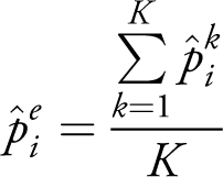
In ViEWS, the ensemble forecast probability ${\hat{p}}_{i}^{e}$ for observation i is currently the unweighted average prediction from all K models:⁸

{\hat{p}}_{i}^{e} = \frac{\sum_{k = 1}^{K} {\hat{p}}_{i}^{k}}{K}

The cm ensemble consists of the 8x3 models listed in Table II (8 models estimated using dynamic simulation, one-step-ahead logits, and random forests). Moreover, the pgm ensemble includes the 10x3 models listed in Table III, again estimated in three different ways. The full list of models and evaluation of each model included in the ensembles is shown in Appendix sections G, H, and I.

Cross-level representation: Combining two levels of analysis

The risk of conflict in a given location is influenced by local factors as well as country-level factors. ViEWS aims to make the two levels of analysis inform each other. Our pgm model ensemble currently combines three approaches. The first approach is to ignore cm factors. The second is to add core cm variables to the pgm model specification. This approach may be suboptimal, however, since it tends to spread the country-level risk evenly out across the country’s territory. This may lead the model to over-predict in low-risk locations even when our pgm models are able to differentiate between the local risk levels. To counter this, we also include as a third approach some models that are based on the product of the predicted probabilities at the cm and pgm levels.

Handling of missing or incomplete data

Dependent variables

In about 15% of the cases, UCDP-GED is unable to precisely identify the location of conflict. ViEWS has developed a method for multiple imputation of imprecise conflict locations that considerably improves the predictive performance of the system. The method employs the locations of precisely known events within the same conflict and within close temporal proximity to determine a spatial probability distribution of latent conflict propensity for each uncertain event. See Croicu & Hegre (2018) and Appendix F.1 for details.

Predictor variables

The methods in ViEWS require that the input data used for the simulations and predictions are complete. Dropping observations with missing values would make it impossible to make predictions for those observations. If the data cannot be assumed to be missing completely at random, dropping them creates bias in parameter estimates and standard errors of the models (Allison, 2009), and presumably also in forecasts. To counter this issue, we perform multiple imputation to replace the missing data using the Amelia II package in R (Honaker, King & Blackwell, 2011). We provide more details in Appendix F.2.

Projections

To generate forecasts for the future, the system requires that the input predictor matrix $X_{t}^{(k)}$ is defined for all the timesteps t over the forecast window. ViEWS will make use of three strategies to project these input predictors.

The first is to use our dynamic forecasting system (see the ‘Dynamic simulation’ section). The forecasts we generate for state-based conflict or any other endogenous variable at t are used as projected inputs in each relevant equation at t + 1. A similar approach can be used for other events. For instance, dynamic simulations of ACLED protest events (Raleigh et al., 2010) are used as projections in models that include protest variables. The second is to use information from external sources. This is often straightforward: most countries, for instance, have scheduled dates for elections over the next few years. We will also search for projections for other predictors such as droughts in a given location, or expected growth rates for a given country. The third is to make very simple assumptions, for example that a predictor is unchanged over the forecasting window. This approach is the one we use for most predictors in the system.

How well do we predict? Evaluation of models

To evaluate the out-of-sample predictive performance of the ViEWS forecasting system, we use the ‘evaluation periodization’ (Table IV). We evaluate by comparing predictions based on data from the training and calibration periods with what the UCDP observed in the testing period.⁹

Principles and metrics for model evaluation

We evaluate our models using four metrics: area under the curve of the receiver operating characteristic (AUROC), area under the precision-recall curve (AUPR), Brier score, and accuracy. The AUROC and AUPR metrics range from 0 to 1, with high values signifying good predictive performance. AUROC is based on the ROC curve, which plots the true positive rate¹⁰ ( $T P R = \frac{T P}{T P + F N}$ ) over the true negative rate ( $T N R = \frac{T N}{F P + T N}$ ) for each possible threshold.¹¹ AUROC scores are high for models that correctly recall a large fraction of the positives for any given level of false alarms. AUPR is based on the PR plot, which plots precision ( $P r = \frac{T P}{T P + F P}$ ) over recall ( $R = \frac{T P}{T P + F N}$ ).¹² AUPR scores are high for models that are correct in a large fraction of the positive predictions for any given level of recall or true positive rate. The Brier score is defined as

B S = \frac{1}{N} \sum_{i = 1}^{N} {({\hat{p}}_{i} - A_{i})}^{2}

where

{\hat{p}}_{i}

is the prediction for observation i and

A_{i}

what actually occurred. Brier scores range from 0 to 1, and lower scores correspond to better performance. Accuracy (A) is the proportion of cases that are correctly classified:

Table V.

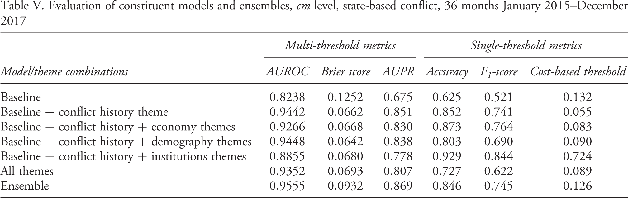
Evaluation of constituent models and ensembles, cm level, state-based conflict, 36 months January 2015–December 2017

Model/theme combinations	Multi-threshold metrics			Single-threshold metrics
Model/theme combinations	AUROC	Brier score	AUPR	Accuracy	F₁-score	Cost-based threshold
Baseline	0.8238	0.1252	0.675	0.625	0.521	0.132
Baseline + conflict history theme	0.9442	0.0662	0.851	0.852	0.741	0.055
Baseline + conflict history + economy themes	0.9266	0.0668	0.830	0.873	0.764	0.083
Baseline + conflict history + demography themes	0.9448	0.0642	0.838	0.803	0.690	0.090
Baseline + conflict history + institutions themes	0.8855	0.0680	0.778	0.929	0.844	0.724
All themes	0.9352	0.0693	0.807	0.727	0.622	0.089
Ensemble	0.9555	0.0932	0.869	0.846	0.745	0.126

A = \frac{T N + T P}{T N + F P + F N + T P}

. The accuracy metric differs from the other three in that it is defined for only a single threshold. We select the threshold that minimizes the misclassification costs in the calibration period of the models we evaluate (see Appendix G for details).

We use multiple performance metrics because model performance is multidimensional. In many model comparisons, one model outperforms others in terms of all measures, so we can safely conclude on the best. In other situations, the picture is less consistent and multiple metrics reflect this. In particular, while the Brier score favors sharp, accurate probabilistic predictions (near 0 or 1), the relative ordering of the forecasts are used for AUROC and AUPR. Moreover, since the AUROC captures the trade-off between producing a large number of true positives versus the expense of many false alarms, the metric favors models that are good at correctly predicting no-conflict cases. The AUPR, on the other hand, focuses on the positive cases, since it captures the trade-off between maximizing the proportion of positive predictions that are correct versus identifying as many of the actual conflicts as possible. Consequently, the AUPR does not reward models that only excel at predicting non-conflict cases. Since we are more interested in predicting instances of political violence than the absence of such, we give priority to the AUPR over the AUROC, as the former rewards models more for accurately predicting conflict rather than non-conflict.

Overall performance

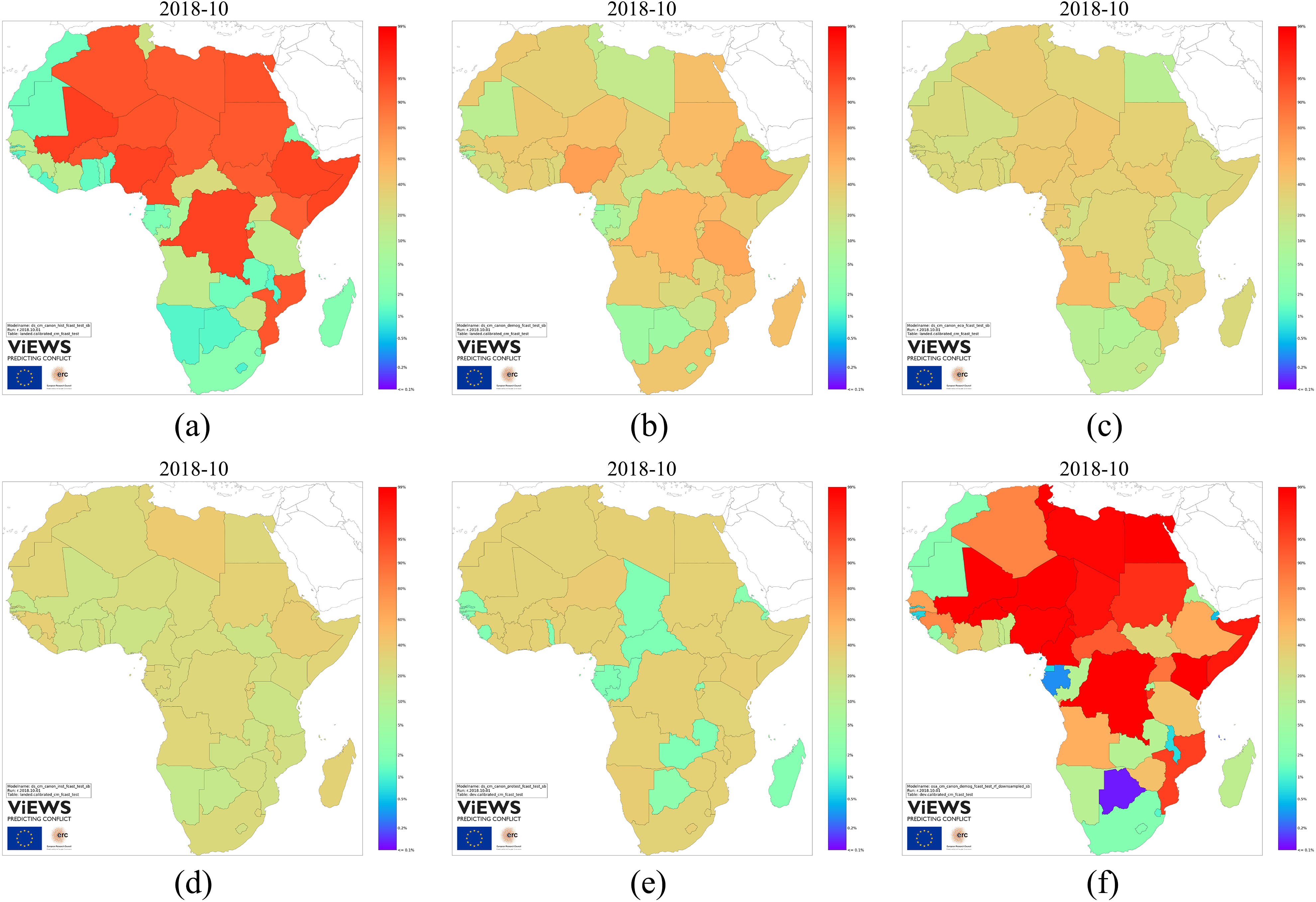
Table V shows summary statistics of the predictive performance of the ViEWS forecasts for state-based conflict at the cm level aggregated over the test period (2015–17).¹³ Since the metrics introduced above depend on the data they are applied to, they are most informative when compared to a baseline prediction for the same forecasting problem. The top line reports our metrics for the baseline model defined above (Table II). The following lines report the same for a set of reference models that include an increasing number of themes from Table II. Note that our final ensemble does not include all these models – they are only used here to demonstrate the relative importance of the themes.¹⁴

The second line in Table V combines the baseline and the conflict history theme predictors. Adding conflict history to the baseline model increases AUROC from 0.824 to 0.944, AUPR from 0.675 to 0.851, and reduces the Brier score from 0.125 to 0.066. Accuracy and F₁ score given the optimal threshold also increases. The three middle lines in the table show the relative contribution of the three main cm-level themes: economics, demography, and institutions. In isolation, they have ambiguous contributions to the baseline + conflict history model: the precision-recall curve deteriorates for all models, and the other metrics improve only for the demography model.

Finally, we turn to the evaluation of the cm ensemble, displayed in the final row in Table V. The metrics show that the ensemble increases the predictive performance considerably in comparison to the baseline models. Compared to the model including the demography theme, there is an increase in AUROC from .9448 to .9555 and in AUPR from .838 to .869. The Brier score, on the other hand, worsens from 0.0642 to 0.0932. This may be because the ensemble model yields more high-probability predictions than the simpler models, and these are punished excessively by the Brier score.

Table VI.

Evaluation of constituent models and ensembles, pgm level, state-based conflict, 36 months January 2015–December 2017

Model/theme combinations	Multi-threshold metrics			Single-threshold metrics
Model/theme combinations	AUROC	Brier score	AUPR	Accuracy	F₁-score	Cost-based threshold
Baseline	0.6324	0.00657	0.049	0.994	0.159	0.017
Baseline + conflict history theme	0.8920	0.00718	0.225	0.988	0.262	0.066
Baseline + conflict history + social and natural geography themes	0.9225	0.00676	0.227	0.992	0.278	0.141
All themes	0.9125	0.00650	0.245	0.990	0.254	0.110
Ensemble	0.9484	0.00623	0.277	0.991	0.289	0.064

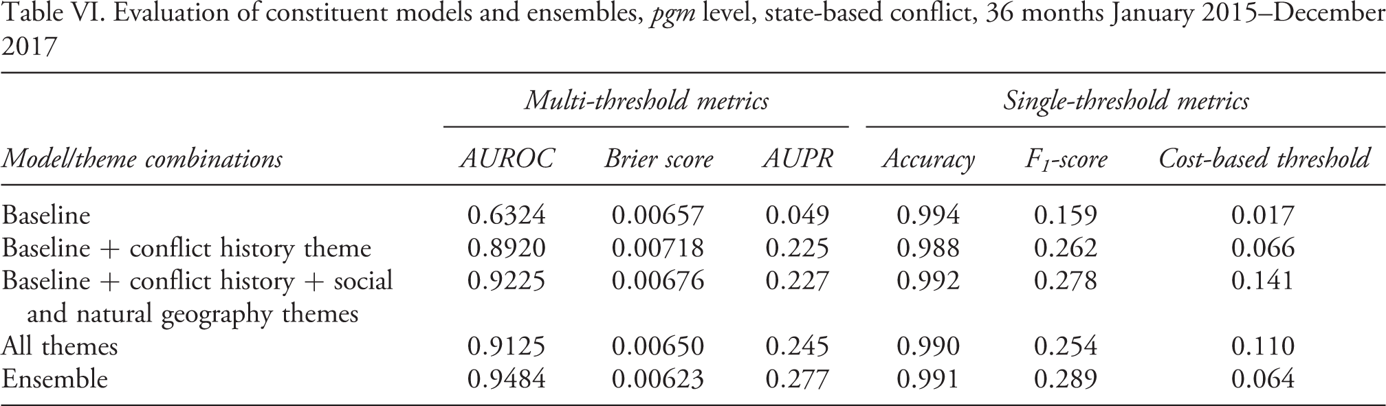
The evaluation for the pgm level is summarized in Table VI. Adding the conflict history theme to the baseline model represents a huge improvement in terms of both AUROC and AUPR, but not so in terms of Brier scores. Adding the two geographical themes improves performance in terms of all metrics. When we add the cm predictors to the models, the AUROC deteriorates whereas the other two improve. This indicates that cm-level predictors are important also at the fine-grained geographical level, but involves a certain ‘smearing’ cost – this model simply lifts the pgm-level probabilities up uniformly within high-risk countries, partly ignoring the local information in the simpler models.

The ensemble, again, performs much better than the constituent parts across all metrics. Compared to the conflict history model, the ensemble improves AUROC from 0.892 to 0.948, AUPR from 0.225 to 0.277, and Brier score from 0.00718 to 0.00623. These improvements are considerable. The ensemble successfully sorts observations into higher and lower probability and thus improves AUROC and AUPR. At the same time, the modest improvement in the Brier score shows that the value of the ensemble predicted probabilities for true positives is still quite far from 1. In other words, compared to the baseline models, the ensemble is not making sharper predictions that clearly separate the classes.

Overall, however, these evaluations show that the current system does well relative to the baseline models. As ViEWS moves forward, the metrics reported here for the ensemble models will constitute the baselines for future comparisons. These numbers also constitute a new frame of reference for other research aiming to gauge the performance of similar conflict early-warning systems.

Performance over time

The results above implicitly assume that the uncertainty of the forecasts for 2021 is similar to those for 2018, which may be unreasonable. Figure 4 shows how the predictive performance of the ViEWS forecasts change depending on how far into the future we move. As before, forecasts for, say, January 2016 are compared with actual outcomes in January 2016, but here we look at the metrics computed for individual months. These evaluations enable us to gauge the feasibility of forecasting up to 36 months into the future. The top row shows performance for the conflict outcomes at the cm level, the bottom row the same for pgm. In the plots in the left column, the y axis shows AUROC for each month and the right column AUPR. Since the predictive performance differs between the models, the y axis varies from plot to plot. The x axis shows the month of the forecast, moving from one to 36 months into the future. The lines are smoothed using a loess function.¹⁵

At the cm level, both AUROC and AUPR decline over time. As we move further into the future, it becomes increasingly difficult to predict accurately. The deterioration is substantial, especially for AUPR. In the top left figure, AUROC decreases from about 0.98 in the first six months to around 0.95 in the second and third years. Top right, we also see a decrease in AUPR. In the first six months, AUPR is well over 0.90. In the second and third years, it is closer to 0.80 on average. More strikingly, AUROC and AUPR at the pgm change much less over time. In the third year of the forecasting window, the system still retains an AUPR at about 0.25. This is probably because of the quite static conflict picture across Africa. In Appendix B.3 we show how persistent the patterns have been throughout the later training and calibration periods and up to today. The results

Figure 4.

Performance for model ensembles over time, cm (top) and pgm (bottom)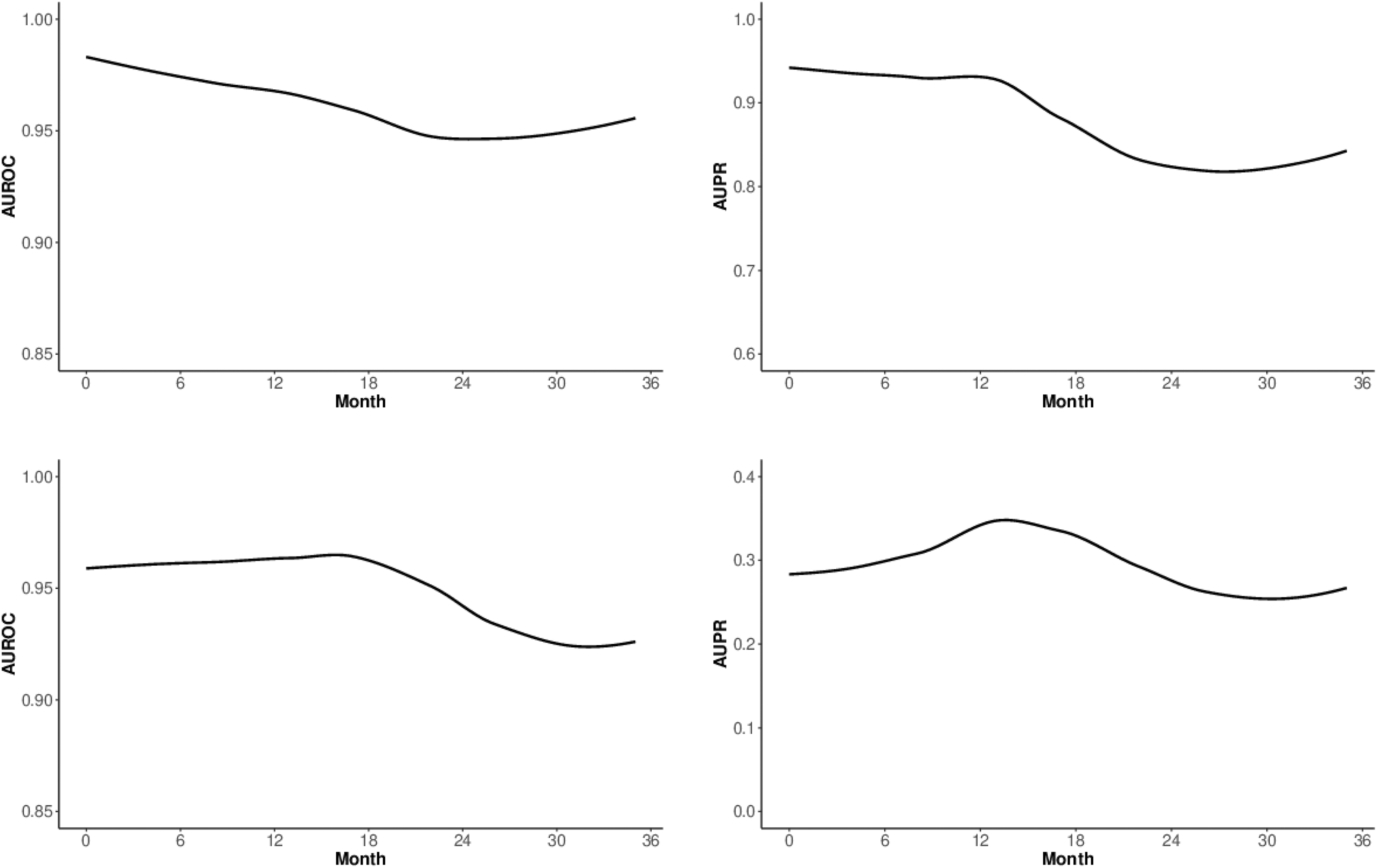

consolidate our expectation that the ViEWS forecasts perform better in the near than the distant future, but that forecasting over a three-year horizon is fully within reach. This evaluation also sets the standard against which ViEWS will improve performance.

Current forecasts

Here, we present the ViEWS forecasts as of 1 October 2018. These are the first set of results using the model setup described in the previous sections. Since June 2018, we have published updated forecasts for the coming 36 months at http://views.pcr.uu.se/ and are continuously updating.¹⁶

State-based conflict sb

Figure 5 shows the current ensemble forecasts for sb conflict – based on our cm-level (left) and pgm-level ensembles (right). They show the forecasts for the immediate future – what will happen in October 2018? Since our ensembles aggregate the constituent models, they closely reflect the insights drawn above from Figures 2 and 3. At the cm level (left figure), our results are in line with mainstream studies. For instance, we forecast a high probability of sb conflict in countries with large populations (Fearon & Laitin, 2003; Raleigh & Hegre, 2009), in non-democracies and countries with recent regime change (Hegre et al., 2001; Cederman, Hug & Krebs, 2010), with low or negative growth rates (Collier & Hoeffler, 2004), and with low education levels (Thyne, 2006) or other indicators of low socio-economic development.

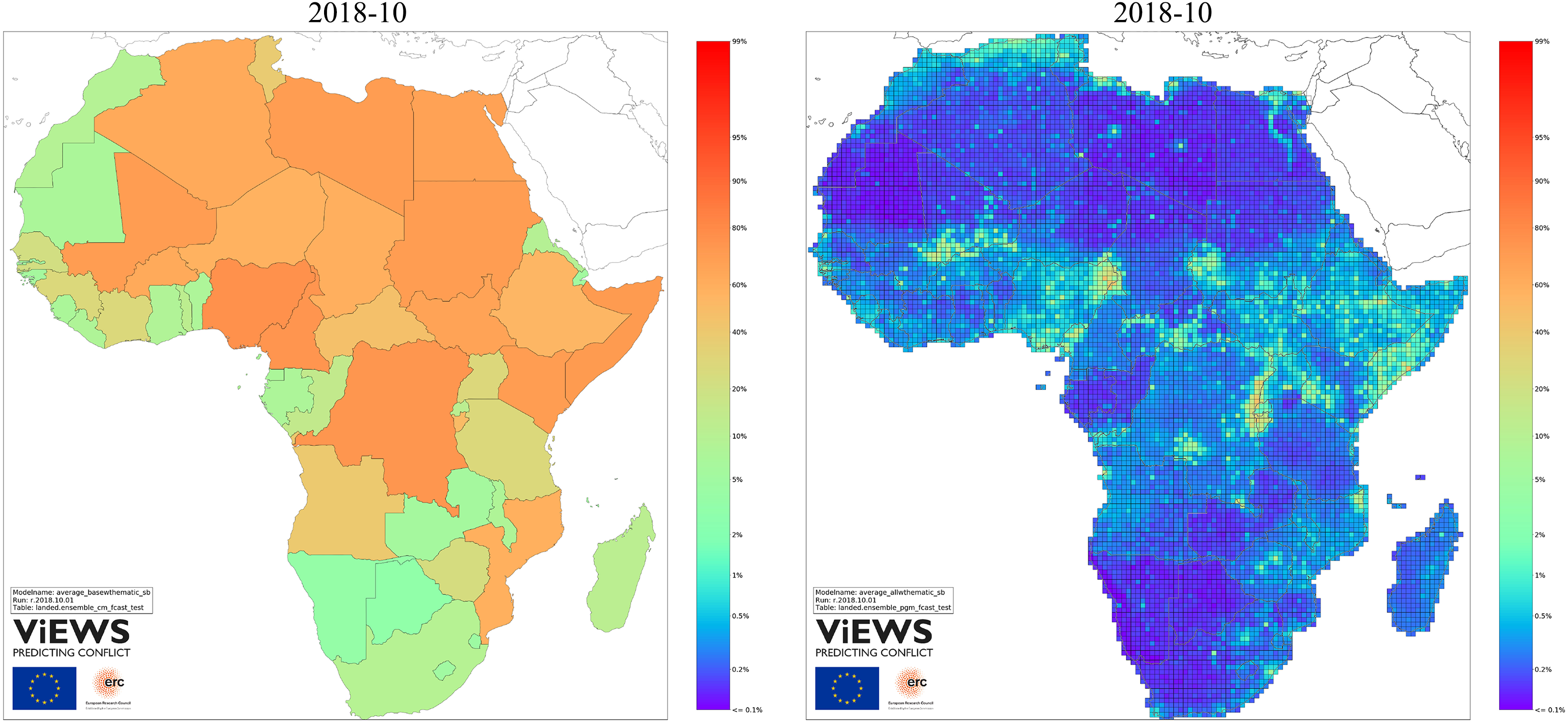
Comparing Figure 5 with the observed conflict history reproduced in Appendix B.2, it is clear how a recent history of conflict translates into a high probability of conflict. In Mali, Nigeria, and DR Congo conflict is almost certain. We also forecast a high probability of state-based conflict (sb) in south-west Cameroon, driven by recent events. Tensions and violence have escalated since separatists symbolically declared independence of ‘Ambazonia’ in October 2017. The separatist violence, involving several groups, continued in 2018 (Crisis Watch, 2018a). There have also been clashes between government forces and IS/Boko Haram in the northern part of the country.¹⁷

Figure 5.

ViEWS forecasts for state-based conflict, October 2018

The rightmost map in Figure 5 shows ViEWS forecasts for statebased conflict at the pgm level. The color mapping is the same as for the cm forecasts. The densest risk clusters for state-based conflict are in northern Nigeria, the Kivu provinces in DRC, Somalia, and Darfur. All of these regions have been ravaged with violence for years. These maps reflect that countries’ recent conflict history is the strongest predictor of future violence. The 2017 re-activation of armed conflict between the government and Renamo de-escalated markedly as talks moved forward during the spring and summer of 2018 (Crisis Watch, 2018b). At the same time, we also see a surge in conflict in the north east where government forces clashed with suspected Islamist militants during the summer of 2018. The militants also increased their attacks against civilians during the summer (allAfrica, 2018).

Beyond history, our natural and social geography features are also important. The low population concentration in Sahara translates into a low risk of conflict, and conflicts are more likely in border regions than close to countries’ capitals. The maps also show how country-level risk assessments influence the geographical forecasts. Zambia, Botswana, and Tanzania, for instance, have markedly lower probability of future conflict than neighboring countries.

All forecasts shown so far have been for October 2018, the second month after the most recent data available. Figure 6 indicates how the forecasts change over time. The color mapping is roughly the same as above, but here corresponds to the forecasted proportion of PRIO-GRID cells in sb conflict for each country. In Burundi, for instance, we expect about 18% of the cells to have conflict in each month. In Ethiopia, the forecast is 1.2%.

Our models reflect that forecasted violence in these clusters change little over time – most countries have the same color throughout the period.¹⁸ This reflects that our projections for the exogenous variables change little, which may artificially inflate the impression of constant future conflict. But the predicted persistence is also reflecting patterns that are very real. The ViEWS models contain information about conflict events many years into the past, and the underlying estimates indicate that African conflicts in general are very persistent (see Appendix B.3). Consequently, most of the variation in Figure 6 is between countries, not across time, and there is only a very slight tendency of a ‘regression to the mean’.

There are a couple of exceptions to this static picture. For example, compared to our forecasts a few months ago, we now predict a lower danger of conflict in Togo as the impact of violent events in 2017 recedes (Zodzi, 2017). On the other hand, there is an increasing danger of conflict in DRC and Burundi spilling over into Rwanda. The forecasted proportion of pgms with conflict in Rwanda increases from 0.063 in October 2018 to 0.112 in late 2021.¹⁹

Figure 6.

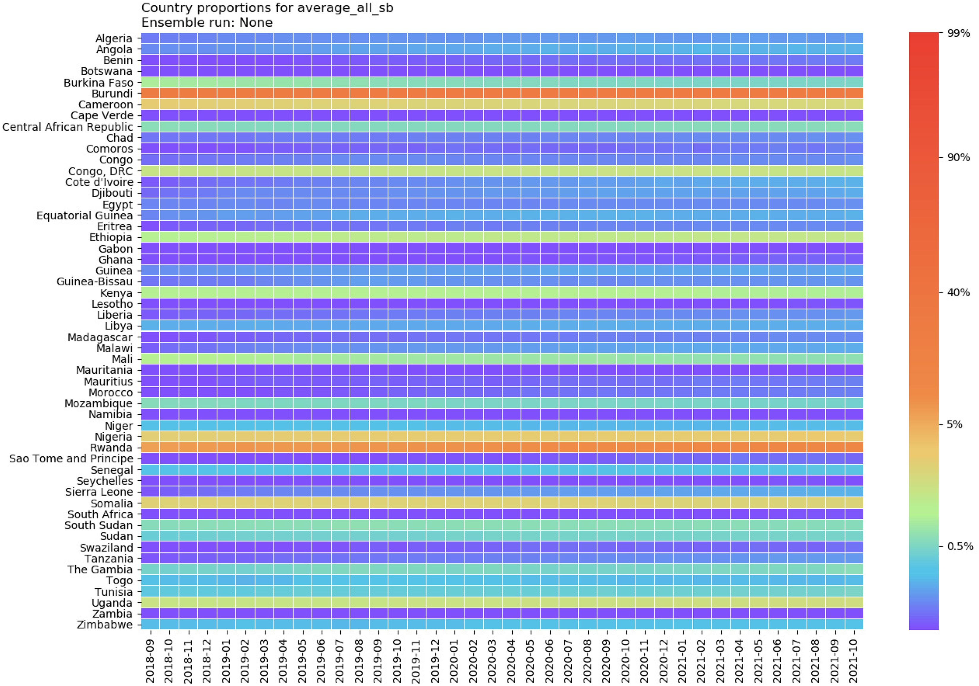
Forecasted proportion of pgm cells with conflict events, by country, September/October 2018–October 2021

Figure 7.

ViEWS forecasts, non-state conflict (left) and one-sided violence (right)

The other two types of outcomes

Figure 7 shows the forecast maps for non-state conflict (ns) and one-sided violence (os). These follow partly the same patterns as sb. Our forecast for ns depends on the same factors as for sb, but seems less suppressed by democratic institutions and socio-economic development than sb events. More importantly, the patterns of past events differ across conflict types (see figures in Appendix B.2). Cameroon and Egypt, for instance, have not had much ns conflict, whereas Libya has seen a lot. We forecast a high probability also of ns in Kenya due to recent confrontations between cattle rustlers and herders.

The forecasts for os respond to about the same factors, but are less clearly related to protests and regime change. They also occur more frequently in newly independent countries. Kenya, again, will see continued one-sided violence, most likely perpetrated by the Al-Shabaab.²⁰ At the geographical level, the forecasts for non-state conflict and one-sided violence depend on the same factors although with somewhat different implications. For ns, we forecast main clusters in central Nigeria, Central African Republic, North Kivu, Darfur, and the Kenyan Rift Valley. For os, northern Nigeria, Darfur, North Kivu, and Burundi are the primary hotspots.

Conclusions

This article has presented initial results from the ViEWS forecasting system and summarized the methodology behind these forecasts. We have accounted for the evaluation procedures of ViEWS and established a frame of reference and a baseline that we can compare future extensions to. The evaluation indicates that the system generates very accurate forecasts for conflict-prone regions in Africa.

ViEWS is being developed according to four guiding principles: public availability, uniform coverage, transparency, and methodological innovation. Public availability is ensured by the complete release of all data and procedures on the ViEWS website. This means that ViEWS is restricted to using data that are publicly available, even if predictive performance could be improved by the inclusion of other data. ViEWS safeguards uniform coverage by relying on the UCDP suite of datasets, which consistently applies a clearly articulated definition and procedures that minimize the risk of overseeing conflict.

Transparency and replicability are essential objectives for ViEWS. They are also challenging given the complexity of the system. The system is primarily documented in this article and the accompanying Online appendix. Interested readers can find additional details and updates to the system in auxiliary documentation available on our website. The ViEWS source code is available at https://github.com/UppsalaConflictDataProgram/OpenViEWS. The ViEWS team welcomes any interested party to use the replication material and compare it to their own forecasts.

As we continue to develop ViEWS, we will follow the guidelines of Colaresi & Mahmood (2017), iteratively evaluate the current system, and use this to inform the next generation. We will work to strengthen the ‘early-warning’ component by defining a useful definition of ‘onset’ and partially optimize the system for forecasting such onsets, add assessments of the likely severity of the violence, introduce actors as units of analysis, solicit qualititative input from country experts, and add more predictors that we find can strengthen the forecasting performance.²¹ To document this, we are making change logs avaliable at https://github.com/UppsalaConflictDataProgram/OpenViEWS/blob/master/CHANGELOG.md.

How useful is the current system? Currently, the main strength of ViEWS is not its ability to forecast entirely new conflicts. Still, the system models geographical diffusion quite well. Because of its vicinity to the various conflicts in Nigeria, the recent tensions in Cameroon are reflected as a high predicted probability of further violence. Moreover, the models show how persistent organized violence is in Africa. Our results indicate that the major conflict clusters in Africa will continue to be very violent over the coming three-year period.

Many governments have their own intelligence systems upon which they act in response to threats of organized violence. Such intelligence is never publicly available. If an open-source early-warning system such as ViEWS can be made sufficiently accurate, critical voices may in some cases use this to challenge the assessments government actions are based on. Moreover, outside observers that lack such inside information may use high-quality forecasts to closely monitor a situation, engage in public debate around the risks involved, and possibly take action. NGOs can apply pressure on conflict actors or prepare for humanitarian assistance. Large organizations such as the UN may use the forecasts when they decide on whether to deploy peacekeeping operations (Hegre, Hultman & Nygård, 2019).

Can the system be misused? A government that sees our risk assessment for a location inside the territory it governs might conceivably be led to violently pre-empt the conflict. We do not believe this is a great danger. Local governments have much better information about what is going on than any system based on open-source data can deliver.

ViEWS is currently restricted to Africa, and all models have been trained on Africa-only data. We believe the system can easily be scaled up to global coverage. Most of the results for the country-level thematic models are consistent with previous research done with global data. Some of the geographical features, on the other hand (e.g. distance to diamond deposits), are more specific to Africa. Our intuition is that most of the models specified here translate well outside Africa, but such an extension would probably accentuate the need for more context-sensitive models (e.g. random-slope models). We have, for instance, noted the very persistent and localized conflict patterns in Africa. Other regions may display other patterns, and a global ViEWS would probably benefit from modeling them as conditional either on the regions they take place in or some predictor that affects the dynamics (e.g. general income levels).

We see ViEWS as a step towards a future where high-resolution forecasts of conflict at practically useful spatial and temporal scales are publicly available. While any such system for violence will necessarily be less precise than those for physical systems, the goal is to improve outcomes relative to a world where these forecasts do not exist. Even an imperfect future system has the potential to inform the placement of peacekeepers, the deployment of NGO resources, and even the decisions of private citizens. Making it more difficult to hide behind a cover of ignorance may potentially save lives. Attaining this goal will take a community of researchers collaborating across domain specialties to identify mistakes, suggest innovations, and incorporate successful new ideas into a computational infrastructure. We believe ViEWS is a start towards bringing this vision to fruition.

Footnotes

Replication data and source code

Replication data, the Online appendix, and datasets with detailed predictions are available at http://views.pcr.uu.se/downloads/. Full source code is available at .

Acknowledgements

The authors would like to thank the anonymous reviewers, Allan Dafoe, Nils Metternich, Nils Weidmann, and numerous participants in several seminars where this work has been presented. For more information on the project see .

Funding

ViEWS receives funding from the European Research Council (ERC) under the European Union’s Horizon 2020 research and innovation programme (grant agreement no. 694640) as well as from Uppsala University. ViEWS computations are performed on resources provided by the Swedish National Infrastructure for Computing (SNIC) at Uppsala Multidisciplinary Center for Advanced Computational Science (UPPMAX).

ORCID iD

Håvard Hegre

Hanne Fjelde

Desirée Nilsson

Notes

References

allAfrica (2018) Togo: One person killed as Togolese opposition resume protests amidst another crackdown (https://allafrica.com/stories/201804250679.html).

Allansson

Marie

Melander

Erik

Themnér

Lotta

(2017) Organized violence, 1989–2016. Journal of Peace Research 54(4): 574–587.

Allison

Paul D

(2009) Missing data. In: Millsap

Roger E

Maydeu-Olivares

Alberto

(eds) The SAGE Handbook of Quantitative Methods in Psychology. London: Sage, 72–90.

Andriole

Stephen J

Young

Robert A

(1977) Toward the development of an integrated crisis warning system. International Studies Quarterly 21(1): 107–150.

Armstrong

J Scott

(2001) Combining forecasts. In: Scott Armstrong

(ed.) Principles of Forecasting. Springer, 417–439.

Brandt

Patrick T

Freeman

John R

Schrodt

Philip A

(2011) Real time, time series forecasting of inter- and intra-state political conflict. Conflict Management and Peace Science 28(1): 41–64.

Brandt

Patrick

Schrodt

Philip

Freeman

John

(2014) Evaluating forecasts of political conflict dynamics. International Journal of Forecasting 30(4): 944–962.

Breiman

Leo

(2001) Random forests. Machine Learning 45(1): 5–32.

Bueno de Mesquita

Bruce

(2010) The Predictioneer’s Game: Using the Logic of Brazen Self-Interest to See and Shape the Future. New York: Random House.

10.

Buhaug

Halvard

Gates

Scott

(2002) The geography of civil war. Journal of Peace Research 39(4): 417–433.

11.

Buhaug

Halvard

Cederman

Lars-Erik

Rød

Jan Ketil

(2008) Disaggregating ethno-nationalist civil wars: A dyadic test of exclusion theory. International Organization 62(3): 531–551.

12.

Buhaug

Halvard

Gates

Scott

Lujala

Päivi

(2009) Geography, rebel capability, and the duration of civil conflict. Journal of Conflict Resolution 53(4): 544–569.

13.

Buhaug

Halvard

Levy

Jack S

Urdal

Henrik

(2014) 50 years of peace research: An introduction to the Journal of Peace Research anniversary special issue. Journal of Peace Research 51(2): 139–144.

14.

Cederman

Lars-Erik

Gleditsch

Kristian Skrede

(2009) Introduction to special issue on disaggregating civil war. Journal of Conflict Resolution 53(4): 487–495.

15.

Cederman

Lars-Erik

Hug

Simon

Krebs

Lutz F

(2010) Democratization and civil war: Empirical evidence. Journal of Peace Research 47(4): 377–394.

16.

Cederman

Lars-Erik

Wimmer

Andreas

Min

Brian

(2010) Why do ethnic groups rebel? New data and analysis. World Politics 62(1): 87–119.

17.

Chiba

Daina

Gleditsch

Kristian Skrede

(2017) The shape of things to come? Expanding the inequality and grievance model for civil war forecasts with event data. Journal of Peace Research 54(2): 275–297.

18.

Colaresi

Michael

Mahmood

Zuhaib

(2017) Do the robot: Lessons from machine learning to improve conflict forecasting. Journal of Peace Research 54(2): 193–214.

19.

Collier

Paul

Hoeffler

Anke

(2004) Greed and grievance in civil war. Oxford Economic Papers 56(4): 563–595.

20.

Collier

Paul

Hoeffler

Anke

Söderbom

Måns

(2004) On the duration of civil war. Journal of Peace Research 41(3): 253–273.

21.

Coppedge

Michael

Gerring

John

Altman

David

Bernhard

Michael

Fish

Steven

Hicken

Allen

Kroenig

Matthew

Lindberg

Staffan I

McMann

Kelly

Paxton

Pamela

Semetko

Holli A

Skaaning

Svend-Erik

Staton

Jeffrey

Teorell

Jan

(2011) Conceptualizing and measuring democracy: A new approach. Perspectives on Politics 9(2): 247–267.

22.

Crisis Watch (2018a) Crisis watch: Cameroon (https://www.crisisgroup.org/crisiswatch/september-2018#cameroon).

23.

Crisis Watch (2018b) Crisis watch: Mozambique (https://www.crisisgroup.org/africa/southern-africa).

24.

Croicu

Mihai

Hegre

Håvard

(2018) A fast spatial multiple imputation procedure for imprecise armed conflict events. Working paper (https://www.pcr.uu.se/digitalAssets/717/c_717328-l_1-k_croicuhegrekgi.pdf).

25.

Croicu

Mihai

Sundberg

Ralph

(2013) UCDP georeferenced event dataset codebook version 4.0 (http://www.pcr.uu.se/research/ucdp/datasets/ucdp_ged/).

26.

Eck

Kristine

Hultman

Lisa

(2007) One-sided violence against civilians in war: Insights from new fatality data. Journal of Peace Research 44(2): 233–246.

27.

Esty

Daniel C

Goldstone

Jack A

Gurr

Ted Robert

Surko

Pamela T

Unger

Alan N

(1995) Working papers: State failure task force report. McLean, VA: Science Applications International Corporation.

28.

Fearon

James D

Laitin

David D

(2003) Ethnicity, insurgency, and civil war. American Political Science Review 97(1): 75–90.

29.

Fjelde

Hanne

Uexkull

Nina von

(2012) Climate triggers: Rainfall anomalies, vulnerability and communal conflict in sub-Saharan Africa. Political Geography 31(7): 444–453.

30.

Géron

Aurélien

(2017) Hands-on Machine Learning with Scikit-Learn and TensorFlow: Concepts, Tools, and Techniques to Build Intelligent Systems. Sebastopol, CA: O’Reilly Media.

31.

Gleditsch

Kristian Skrede

Ward

Michael D

(1999) A revised list of independent states since the congress of Vienna. International Interactions 25(4): 393–413.

32.

Gleditsch

Kristian Skrede

Metternich

Nils W

Ruggeri

Andrea

(2014) Data and progress in peace and conflict research. Journal of Peace Research 51(2): 301–314.

33.

Gleditsch

Nils Petter

Wallensteen

Peter

Eriksson

Mikael

Sollenberg

Margareta

Strand

Håvard

(2002) Armed conflict 1946–2001: A new dataset. Journal of Peace Research 39(5): 615–637.

34.

Goldstone

Jack A

Bates

Robert H

Epstein

David L

Gurr

Ted Robert

Lustik

Michael B

Marshall

Monty G

Ulfelder

Jay

Woodward

Mark

(2010) A global model for forecasting political instability. American Journal of Political Science 54(1): 190–208.

35.

Greenhill

Brian

Ward

Michael D

Sacks

Audrey

(2011) The separation plot: A new visual method for evaluating the fit of binary models. American Journal of Political Science 55(4): 990–1002.

36.

Gurr

Ted Robert

Harff

Barbara

Levy

Marc

Dabelko

Geoffrey D

Surko

Pamela T

Unger

Alan N

(1999) State failure task force report: Phase II findings. Environmental Change & Security Project Report (5) (https://pdfs.semanticscholar.org/c343/feeda994f0355b64c8b6a3e21f6024719249.pdf).

37.

Hegre

Håvard

Sambanis

Nicholas

(2006) Sensitivity analysis of empirical results on civil war onset. Journal of Conflict Resolution 50(4): 508–535.

38.

Hegre

Håvard

Buhaug

Halvard

Calvin

Katherine V

Nordkvelle

Jonas

Waldhoff

Stephanie T

Gilmore

Elisabeth

(2016) Forecasting civil conflict along the shared socioeconomic pathways. Environmental Research Letters 11(5): 054002.

39.

Hegre

Håvard

Croicu

Mihai

Eck

Kristine

Högbladh

Stina

(2018) UCDP-monthly. Monthly updated organized violence data in event and aggregated forms (https://www.pcr.uu.se/digitalAssets/653/c_653796-l_1-k_ucdp_candidate_views_outcomes.pdf).

40.

Hegre

Håvard

Ellingsen

Tanja

Gates

Scott

Gleditsch

Nils Petter

(2001) Toward a democratic civil peace? Democracy, political change, and civil war, 1816–1992. American Political Science Review 95(1): 33–48.

41.

Hegre

Håvard

Hultman

Lisa

Nygård

Håvard Mokleiv

(2019) Evaluating the conflict-reducing effect of UN peacekeeping operations. Journal of Politics 81(1): 215–232.

42.

Hegre

Håvard

Karlsen

Joakim

Nygård

Håvard Mokleiv

Strand

Håvard

Urdal

Henrik

(2013) Predicting armed conflict 2010–2050. International Studies Quarterly 55(2): 250–270.

43.

Hegre

Håvard

Metternich

Nils W

Nygård

Håvard Mokleiv

Wucherpfennig

Julian

(2017) Introduction: Forecasting in peace research. Journal of Peace Research 54(2): 113–124.

44.

Honaker

James

King

Gary

Blackwell

Matthew

(2011) Amelia II: A program for missing data. Journal of Statistical Software 45(7): 1–47.

45.

Jansen

Remco

Croicu

Mihai

Hegre

Håvard

Hoyles

Frederick

Olafsdottir

Gudlaug

Randahl

David

Rød

Espen Geelmuyden

(2018) ViEWS monthly estimates tables, October 2018 (http://files.webb.uu.se/uploader/1576/MonthlyEstimateTables-10.pdf).

46.

Le Billon

Philippe

(2001) The political ecology of war: Natural resources and armed conflicts. Political Geography 20(5): 561–584.

47.

Lujala

Päivi

Gleditsch

Nils Petter

Gilmore

Elisabeth

(2005) A diamond curse? Civil war and a lootable resource. Journal of Conflict Resolution 49(4): 538–562.

48.

Lutz

Wolfgang

Goujon

Anne

Samir

Sanderson

Warren

(2007) Reconstruction of population by age, sex and level of educational attainment for 120 countries 1970–2000. Vienna Yearbook of Population Research 5: 193–235.

49.

Melander

Erik

Pettersson

Therése

Themnér

Lotta

(2016) Organized violence, 1989–2015. Journal of Peace Research 53(5): 727–742.

50.

Montgomery

Jacob M

Hollenbach

Florian M

Ward

Michael D

(2012) Improving predictions using ensemble Bayesian model averaging. Political Analysis 20(3): 271–291.

51.

Muchlinski

David

Siroky

David

Jingrui

Kocher

Matthew

(2016) Comparing random forest with logistic regression for predicting class-imbalanced civil war onset data. Political Analysis 24(1): 87–103.

52.

Muller

Edward N

Weede

Erich

(1990) Cross-national variations in political violence: A rational action approach. Journal of Conflict Resolution 34(4): 624–651.

53.

O’Brien

Sean P

(2002) Anticipating the good, the bad, and the ugly: An early warning approach to conflict and instability analysis. Journal of Conflict Resolution 46(6): 791–811.

54.

O’Brien

Sean P

(2010) Crisis early warning and decision support: Contemporary approaches and thoughts on future research. International Studies Review 12(1): 87–105.

55.

Pettersson

Therése

Eck

Kristine

(2018) Organized violence, 1989–2017. Journal of Peace Research 55(4): 535–547.

56.

Raleigh

Clionadh

Hegre

Håvard

(2009) Population size, concentration, and civil war: A geographically disaggregated analysis. Political Geography 28(4): 224–238.

57.

Raleigh

Clionadh

Hegre

Håvard

Karlsen

Joakim

Linke

Andrew

(2010) Introducing ACLED: An armed conflict location and event dataset. Journal of Peace Research 47(5): 651–660.

58.

Schneider

Gerald

Gleditsch

Nils Petter

Carey

Sabine

(2010) Exploring the past, anticipating the future: A symposium. International Studies Review 12(1): 1–7.

59.

Schrodt

Philip A

(1991) Prediction of interstate conflict outcomes using a neural network. Social Science Computer Review 9(3): 359–380.

60.

Schrodt

Philip A

Davis

Shannon G

Weddle

Judith L

(1994) Political science: KEDS – a program for the machine coding of event data. Social Science Computer Review 12(4): 561–587.

61.

Singer

David J

(1973) The peace researcher and foreign policy prediction. Papers of the Peace Science Society (International) 21: 1–13.

62.

Sundberg

Ralph

Melander

Erik

(2013) Introducing the UCDP georeferenced event dataset. Journal of Peace Research 50(4): 523–532.

63.

Thyne

Clayton

(2006) ABCs, 123s, and the golden rule: The pacifying effect of education on civil war, 1980–1999. International Studies Quarterly 50(4): 733–754.

64.

Tilly

Charles

(1978) From Mobilization to Revolution. Reading, MA: Addison-Wesley.

65.

Tollefsen

Andreas Forø

Strand

Håvard

Buhaug

Halvard

(2012) PRIO-grid: A unified spatial data structure. Journal of Peace Research 49(2): 363–374.

66.

Ward

Michael D

Beger

Andreas

(2017) Lessons from near real-time forecasting of irregular leadership changes. Journal of Peace Research 54(2): 141–156.

67.

Ward

Michael D

Greenhill

Brian D

Bakke

Kristin M

(2010) The perils of policy by p-value: Predicting civil conflicts. Journal of Peace Research 47(4): 363–375.

68.

Weidmann

Nils B

Ward

Michael D

(2010) Predicting conflict in space and time. Journal of Conflict Resolution 54(6): 883–901.

69.

Weidmann

Nils B

Kuse

Doreen

Gleditsch

Kristian Skrede

(2010) The geography of the international system: The CShapes dataset. International Interactions 36(1): 86–106.

70.

World Bank (2015) World development indicators (http://data.worldbank.org/products/wdi).

71.

Wucherpfennig

Julian

Weidmann

Nils B

Girardin

Luc

Cederman

Lars-Erik

Wimmer

Andreas

(2011) Politically relevant ethnic groups across space and time: Introducing the GeoEPR dataset. Conflict Management and Peace Science 28(5): 423–437.

72.

Zodzi

John

(2017) Four killed in Togo as protesters clash with security forces (https://af.reuters.com/article/idAFKBN1CO0Q7-OZATP).