
Abstract
The ubiquitous presence of endogenous regressors presents a significant challenge when drawing causal inferences using observational data. The classical econometric method used to handle regressor endogeneity requires instrumental variables (IVs) that must satisfy the stringent condition of exclusion restriction, rendering it unfeasible in many settings. Herein, the authors propose a new IV-free method that uses copulas to address the endogeneity problem. Existing copula correction methods require nonnormal endogenous regressors: Normally or nearly normally distributed endogenous regressors cause model nonidentification or significant finite-sample bias. Furthermore, existing copula control function methods presume the independence of exogenous regressors and endogenous regressors. The authors’ generalized two-stage copula endogeneity-correction (2sCOPE) method simultaneously relaxes the two key identification requirements while maintaining the Gaussian copula regressor–error dependence structure. They prove that under the Gaussian copula dependence structure, 2sCOPE yields consistent causal-effect estimates with correlated endogenous and exogenous regressors as well as normally distributed endogenous regressors. In addition to relaxing the identification requirements, 2sCOPE has superior finite-sample performance and addresses the significant finite-sample bias problem due to insufficient regressor nonnormality. Moreover, 2sCOPE employs generated regressors derived from existing regressors to control for endogeneity, and can thus considerably increase the ease and broaden the applicability of IV-free methods for handling regressor endogeneity. The authors further demonstrate 2sCOPE's performance using simulation studies and illustrate its use in an empirical application.
Causal inference is central to many problems that both academics and practitioners face. It has become increasingly important as rapidly available observational data in the current digital era promise to offer real-world evidence on cause-and-effect relationships for better decision-making. However, empirical researchers attempting to draw valid causal inferences from these data often encounter the presence of endogenous regressors correlated with the structural error in the population regression model representing the causal relationship of interest. Notably, omitted variables, such as unobserved demand shocks (e.g., product attributes, taste changes), may cause price endogeneity in observational scanner data. Ignoring this endogeneity can yield severely biased estimates of pricing effects on consumer demand (Villas-Boas and Winer 1999).
Instrumental variables (IVs) have traditionally been used to address the endogeneity issue. The ideal IV must satisfy two requirements: First, it must be correlated with the endogenous regressor via an explainable and validated relationship (i.e., relevance restriction), and, second, it must be uncorrelated with the structural error and must not directly affect the outcome (i.e., exclusion restriction). Although the theory of IVs is well-developed, researchers often struggle to find good IVs that meet both criteria. Potential IVs are often deficient by virtue of either weak relevance or challenging justification for exclusion restriction, hindering their use for addressing underlying endogeneity concerns (Rossi 2014).
The development and application of IV-free endogeneity-correction methods to address the lack of suitable IVs have gained traction in recent decades (Ebbes, Wedel, and Böckenholt 2009). Park and Gupta (2012) propose an IV-free method that uses the copula model (Christopoulos, McAdam, and Tzavalis 2021; Danaher 2007; Danaher and Smith 2011) to directly model the regressor–error dependence. 1 In addition to requiring no IVs, the copula approach is straightforward to use: One can simply add the latent copula data for the endogenous regressors as control variables to correct for endogeneity. These features considerably enhance the feasibility of endogeneity correction, as evidenced by the prolific use of the copula correction method (see examples of recent applications noted in the literature review in the next section). Like other IV-free methods, however, the copula correction methods also require distinctiveness between the distributions of the endogenous regressor and the structural error. Assuming Gaussian copula regressor–error dependence, the endogenous regressor is required to have a nonnormal distribution for model identification with the commonly assumed normal structural error distribution (Becker, Proksch, and Ringle 2021; Eckert and Hohberger 2023; Haschka 2022; Papies, Ebbes, and Van Heerde 2017; Park and Gupta 2012; Qian, Koschmann, and Xie 2024; Qian, Xie, and Koschmann 2022). Furthermore, we demonstrate that the existing copula control function correction methods implicitly assume that all exogenous regressors be uncorrelated with the linear combination of copula transformations of endogenous regressors (hereinafter referred to as copula transformed terms, CTT, used in these methods to control for endogeneity) and may yield significant bias when noticeable correlations are present between the endogenous and exogenous regressors.
In practical applications, the requirements of sufficient regressor nonnormality and absence of correlations between endogenous and exogenous regressors can be excessive and pose significant challenges to the application of the copula correction method. We often encounter endogenous regressors or include transformations of endogenous variables as regressors that have close-to-normal distributions. Examples of such regressors in economics and marketing management studies include stock market returns (Sorescu, Warren, and Ertekin 2017), corporate social responsibility (Eckert and Hohberger 2023), the organizational intelligence quotient (Mendelson 2000), and the logarithm of price (see the “Empirical Application” section). Theoretically, the endogenous regressor and the structural error can contain a common set of unobservables that collectively have a normal distribution, which can lead to a close-to-normal distribution of the endogenous regressor. In such scenarios, even if the model is identified asymptotically, the close-to-normality of endogenous regressors can cause estimation bias even in moderate sample sizes and require large sample sizes to mitigate the finite-sample bias (Becker, Proksch, and Ringle 2021). Correlations between the endogenous and exogenous regressors are also common in practical applications, particularly when the exogenous regressors are included to control for potential confounders. Examples of such exogenous control variables abound in marketing and management studies, including customer-specific variables (e.g., location, age, household size, income, past purchase behaviors) when estimating the returns of consumer targeting strategies on product sales (Papies, Ebbes, and Van Heerde 2017) and firms’ similarity when estimating the effect of competition on innovation (Aghion et al. 2005).
The purpose of this article is to provide a generalized copula control function procedure that relaxes the stringent requirements of both sufficient regressor nonnormality and the absence of correlations between endogenous and exogenous regressors. Like the existing copula methods, our proposed two-stage copula endogeneity-correction (2sCOPE) method requires neither IVs nor the assumption of exclusion restriction while assuming the Gaussian copula dependence structure. The 2sCOPE method corrects for endogeneity by adding residuals, obtained by regressing latent copula data for each endogenous regressor on the latent copula data for exogenous regressors, as generated regressors in the structural model. Unlike the original copula method (Becker, Proksch, and Ringle 2021; Eckert and Hohberger 2023; Park and Gupta 2012; hereinafter CopulaOrigin), 2sCOPE can account for the dependence between endogenous and exogenous regressors. CopulaOrigin thus constitutes a special case of 2sCOPE. Assuming that a Gaussian copula correlation model captures dependence among the endogenous regressors, correlated exogenous regressors, and the structural error, we prove that 2sCOPE can identify causal effects under weaker assumptions than CopulaOrigin and overcome the two key limitations mentioned previously.
The remainder of this article begins with a review of relevant literature on methods for causal inference with endogenous regressors and an overview of this work's contributions. We then propose 2sCOPE and prove its consistency with normally distributed and correlated regressors. Next, we evaluate 2sCOPE's performance using simulation studies under different scenarios and provide a flowchart to guide its use in practical applications. We further apply 2sCOPE to estimate price elasticity using store purchase databases.
Literature Review and Contributions
Marketing, economics, and statistics research has developed a rich array of methods for drawing causal inferences. Randomized experiments, such as controlled lab experiments and field experiments (Anderson and Simester 2004; Godes and Mayzlin 2009; Johnson, Lewis, and Nubbemeyer 2017), have long been the gold standard for estimating causal effects. When controlled experiments are not feasible, quasi-experimental designs, such as regression discontinuity, difference-in-difference, and synthetic control, are used to mimic randomized experiments and enable the identification of causal effects with observational data (Athey and Imbens 2006; Hartmann, Nair, and Narayanan 2011; Kim, Lee, and Gupta 2020; Narayanan and Kalyanam 2015; Shi et al. 2017). However, these quasi-experimental designs have special data and design requirements, and are not designed to cope with the general issue of endogenous regressors when estimating causal effects using observational data.
There exists a large literature on various approaches to addressing endogenous regressors when inferring causal effects. Papies, Ebbes, and Van Heerde (2017), Rutz and Watson (2019), and Park and Gupta (2012) provide overviews of approaches to addressing endogeneity in marketing. Among the three broad classes of solutions that they discuss, the most widely employed is the IV approach (Aghion et al. 2005; Ataman, Van Heerde, and Mela 2010; Li and Ansari 2014; Novak and Stern 2009; Qian 2008; Van Heerde et al. 2013). Rossi (2014) surveys a decade of publications in Marketing Science and Quantitative Marketing and Economics and reveals that the most commonly used IVs are lagged variables, costs, fixed effects, and Hausman-style variables from other markets. However, the survey findings show that the IVs’ strengths are rarely measured/reported, despite the necessity of doing so to detect weak IVs. Moreover, the exclusion restriction condition cannot generally be tested to verify the IVs’ validity. The survey findings also show that most articles lack a discussion of why the IVs used are valid. In short, although IVs have a sound theoretical grounding, good ones are difficult to find, making the IV approach difficult to implement in practice.
The second class of solutions for mitigating endogeneity involves specifying the economic structure that generates the observed data on endogenous regressors (e.g., a supply-side model for marketing-mix variables) (Chintagunta et al. 2006; Dotson and Allenby 2010; Otter, Gilbride, and Allenby 2011; Sudhir 2001; Sun 2005; Yang, Chen, and Allenby 2003). A key concern with this approach is that incorrect assumptions or insufficient information on the supply side may generate biased estimates (Chintagunta et al. 2006).
The third class of solutions to endogeneity correction involves IV-free methods, a more recent methodological development. Ebbes, Wedel, and Böckenholt (2009) discuss three extant IV-free approaches: the higher moments approach (Lewbel 1997), the identification through heteroskedasticity estimator (Rigobon 2003), and the latent IV method (Ebbes et al. 2005). Wang and Blei (2019) propose a deconfounder approach that has some flavor of the latent IV approach. All these methods decompose an endogenous regressor into an exogenous part and an endogenous part. The assumption that the endogenous regressor contains an exogenous component that does not directly affect the outcome is akin to the stringent condition of exclusion restriction for observed IVs and thus can be difficult to justify. Park and Gupta (2012) introduce another IV-free method that does not require the stringent condition of exclusion restriction but assumes a Gaussian copula dependence between the structural error and the endogenous regressor. Researchers have enthusiastically adopted the copula method owing to its feasibility without the need for instruments (Atefi et al. 2018; Becker, Proksch, and Ringle 2021; Datta, Foubert, and Van Heerde 2015; Eckert and Hohberger 2023; Elshiewy and Boztug 2018; Haschka 2022; Heitmann et al. 2020). The 2sCOPE contributes to the field by overcoming significant limitations of existing copula correction methods and by virtue of its broader applicability (Table 1).
A Comparison of Copula Correction Methods.
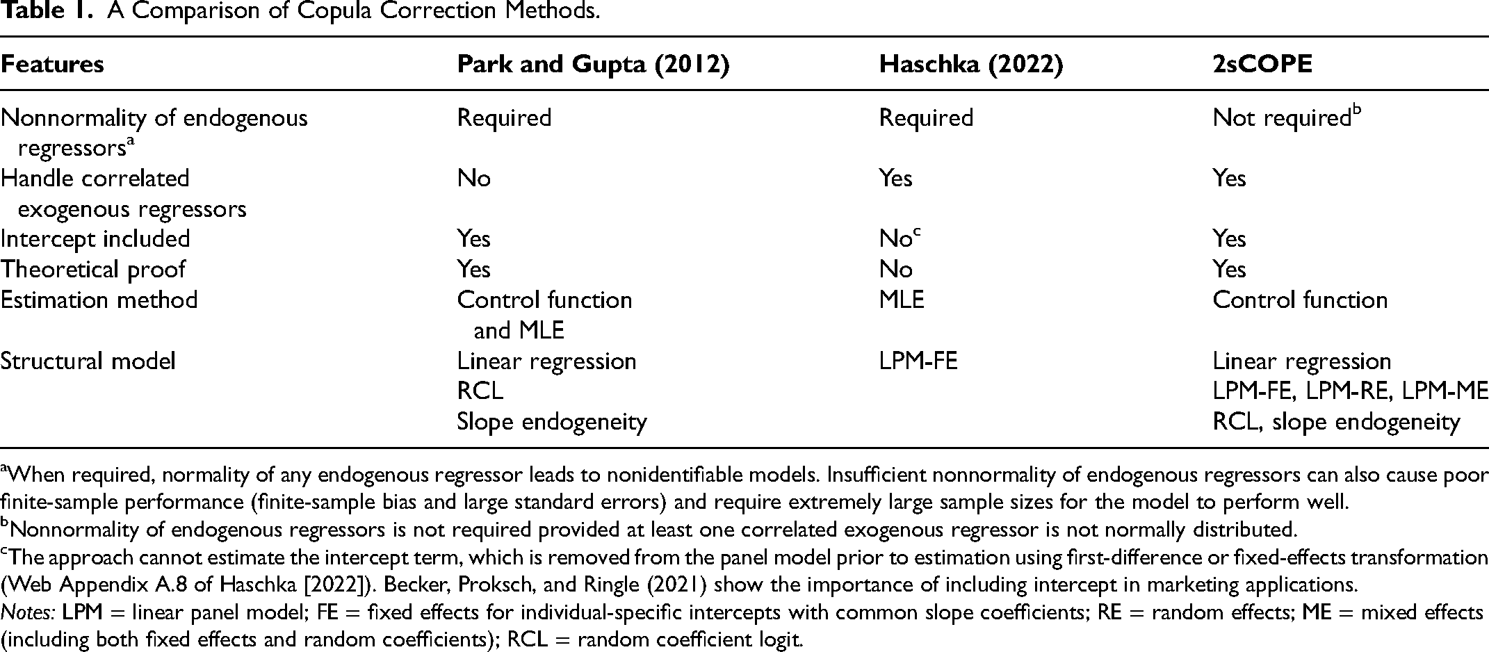
When required, normality of any endogenous regressor leads to nonidentifiable models. Insufficient nonnormality of endogenous regressors can also cause poor finite-sample performance (finite-sample bias and large standard errors) and require extremely large sample sizes for the model to perform well.
Nonnormality of endogenous regressors is not required provided at least one correlated exogenous regressor is not normally distributed.
The approach cannot estimate the intercept term, which is removed from the panel model prior to estimation using first-difference or fixed-effects transformation (Web Appendix A.8 of Haschka [2022]). Becker, Proksch, and Ringle (2021) show the importance of including intercept in marketing applications.
Notes: LPM = linear panel model; FE = fixed effects for individual-specific intercepts with common slope coefficients; RE = random effects; ME = mixed effects (including both fixed effects and random coefficients); RCL = random coefficient logit.
The contributions of 2sCOPE are threefold. First, to our knowledge, this work is novel in providing formal proofs for copula correction methods’ theoretical properties. These theoretical results are necessary given that model identifiability is central to addressing the endogeneity issue. Recent work notes the lack of rigorous proofs of required model identification conditions and estimation properties (consistency and efficiency) for copula correction as a major area requiring further research (Becker, Proksch, and Ringle 2021; Haschka 2022). 2 The theoretical results presented herein help bridge this gap and facilitate a better understanding of the properties of the copula correction methods and their optimal use.
A useful theoretical outcome is that the existence of the correlations between endogenous and exogenous regressors alone does not automatically introduce bias into CopulaOrigin. Rather, we demonstrate that the implicit assumption for CopulaOrigin is the exogenous regressors’ uncorrelatedness with the CTT, the linear combination of copula transformations of endogenous regressors used to control for endogeneity. The difference between the implicit assumption and the condition of zero pairwise correlations between endogenous and exogenous regressors can be substantial, particularly with multiple endogenous regressors. 3 We prove that the proposed 2sCOPE yields consistent causal effect estimates when the preceding implicit assumption is violated, which can cause biased causal effect estimates for CopulaOrigin. Our other novel finding is that although the exogenous regressors that are correlated with the CTT require special handling for consistent causal effect estimation, they can be leveraged efficiently by 2sCOPE to substantially improve the identification and finite-sample performance of copula correction. Significantly, we prove that the structural model with normally distributed endogenous regressors can be identified using 2sCOPE, provided that one of the exogenous regressors correlated with endogenous ones is nonnormal, which is considerably more feasible in many practical applications.
Second, the proposed 2sCOPE method is the first copula correction method that simultaneously relaxes the nonnormality assumption of endogenous regressors and handles correlated endogenous and exogenous regressors (Table 1). Existing copula correction methods do not account for correlated endogenous and exogenous regressors. An exception is that of Haschka (2022), who generalizes Park and Gupta (2012) to fixed-effects linear panel models with correlated regressors by jointly modeling the structural error and endogenous and exogenous regressors using copulas and maximum likelihood estimation (MLE). However, Haschka's approach still requires the nonnormality of endogenous regressors. Thus, all existing copula correction methods require assumption of sufficient nonnormality of endogenous regressors for model identification and acceptable finite sample performance (Becker, Proksch, and Ringle 2021; Eckert and Hohberger 2023; Haschka 2022). Becker, Proksch, and Ringle (2021) suggest a minimum absolute skewness of 2 for an endogenous regressor to ensure good performance of Gaussian copula correction methods in a sample under 1,000 (Figure 8 in Becker, Proksch, and Ringle 2021). These requirements can significantly limit the practical deployment of copula correction methods.
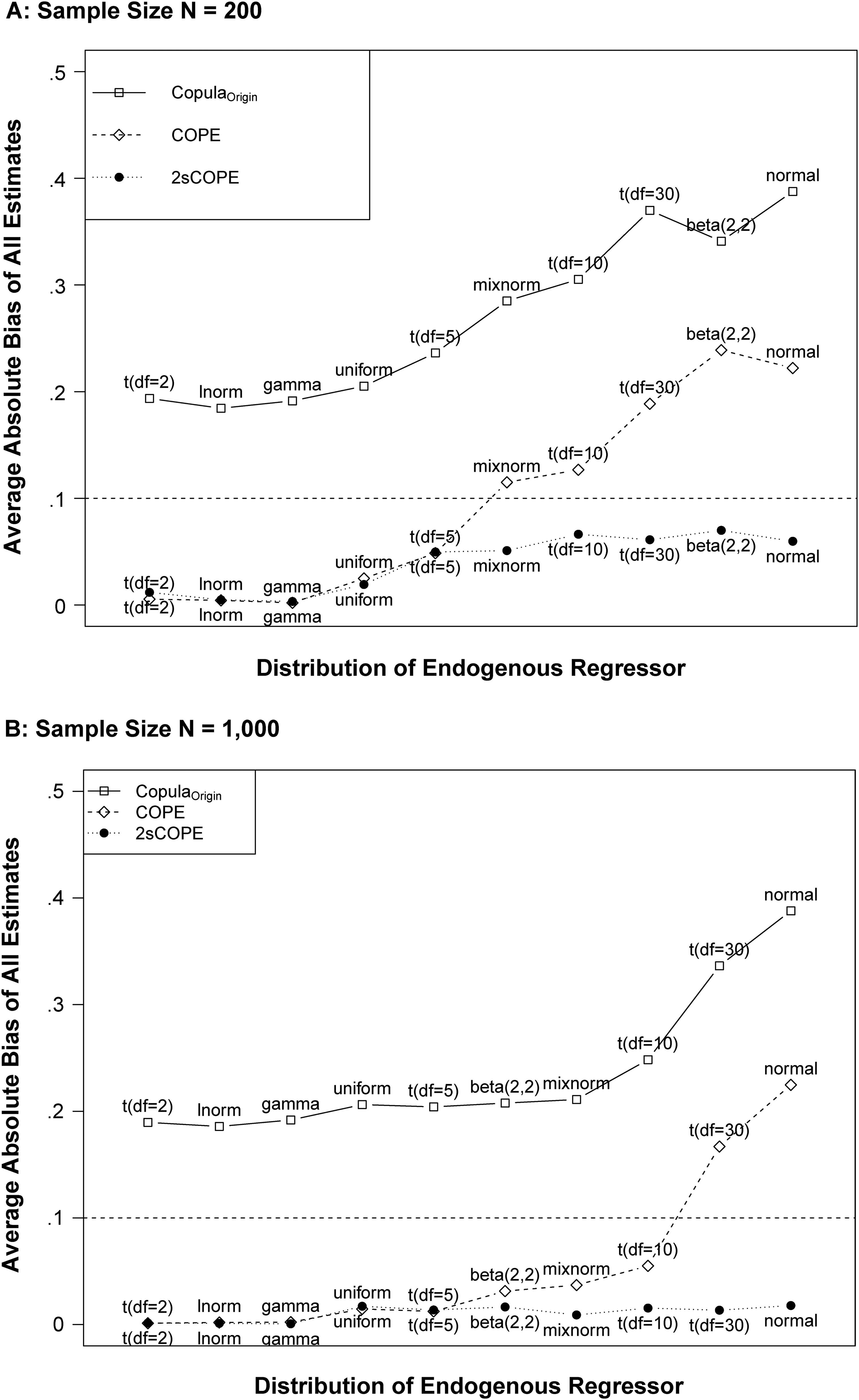
Our proposed 2sCOPE method overcomes these important restrictions of existing copula correction methods. Consistent with our theoretical results, the evaluation in Cases 2 and 3 of the simulation demonstrates the superior finite-sample performance of 2sCOPE and shows that 2sCOPE eliminates or substantially reduces the significant problem of finite-sample bias associated with insufficient regressor nonnormality raised in Becker, Proksch, and Ringle (2021) and Eckert and Hohberger (2023). Even when the endogenous regressor is normal or close-to-normal with a skewness of 0, the estimation bias of 2sCOPE remains negligible for a sample size as small as 200 (Figure 1). We further conduct systematic simulation studies and provide an actionable guideline for using 2sCOPE (Figure 2), establishing sufficient conditions regarding exogenous regressors that are verifiable using tests of nonnormality and relevance to endogenous regressors, to effectively handle endogenous regressors with insufficient nonnormality using data at hand. Overall, 2sCOPE can substantially broaden IV-free methods’ practical applicability for handling endogeneity issues.
Average Absolute Estimation Bias of All Regression Parameters (μ, α, β) in the Structural Model for Different Endogenous Regressor Distributions.
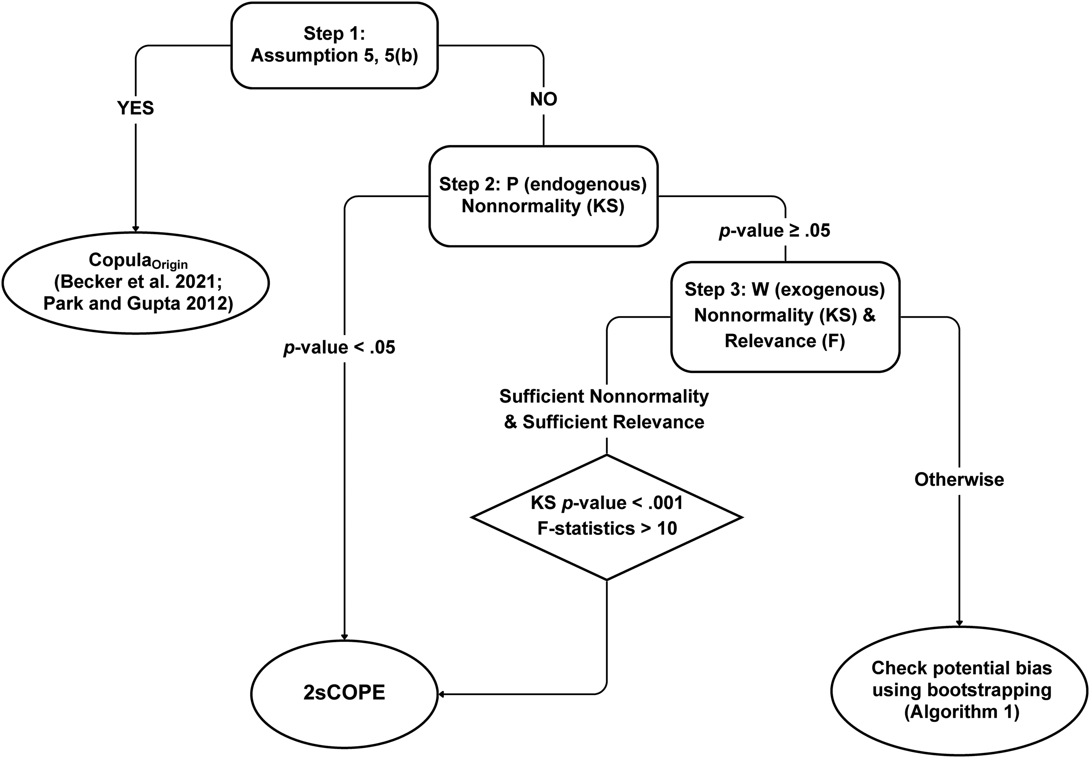
Decision Tree for Using 2sCOPE.
Third, the proposed 2sCOPE provides a versatile and feasible copula control function method for handling regressor endogeneity. Although the vast majority of applications using the copula correction method have employed the generated-regressor approach (Becker, Proksch, and Ringle 2021; Eckert and Hohberger 2023), no existing copula control function method can handle endogenous regressors that have insufficient nonnormality or are correlated with exogenous regressors. The 2sCOPE method addresses this need and enjoys several benefits associated with the control function versus the alternative MLE approach. These include—but are not limited to—little extra computational and modeling burdens to be integrated with complex outcome models commonly used in marketing studies (Table 1), broader applicability with weaker assumptions, and increased robustness to model misspecifications. 4
In many such models, the MLE approach becomes considerably more difficult or computationally infeasible while 2sCOPE is straightforward. Footnote 8 offers an example demonstrating that extension of Haschka's (2022) MLE approach to random coefficient linear panel models with correlated endogenous and exogenous regressors requires the numerical evaluation of potentially high-dimensional integrals of complicated functions containing the product of copula density functions, evaluated at repeated measurement occasions. However, 2sCOPE involves none of these integrals and can be implemented using standard software programs for random coefficient linear panel models, assuming all regressors are exogenous. Furthermore, although 2sCOPE assumes a normal error distribution, we show its robustness to symmetric nonnormal error distributions (see the Web Appendix), in contrast to existing methods’ sensitivity to such error misspecifications (Becker, Proksch, and Ringle 2021). Thus, the 2sCOPE control function approach leveraging correlated exogenous regressors can enhance robustness to model misspecifications.
Methods
In this section, we develop a copula-based IV-free method for handling endogenous regressors with insufficient nonnormality or correlated with exogenous regressors. We first review CopulaOrigin and demonstrate that it implicitly assumes no correlations between exogenous regressors and the CTT as well as the bias in the structural model parameter estimates that may arise from the violation of this assumption. We then propose a new approach to the problem and the detailed estimation procedure. We also demonstrate how exogenous regressors correlated with endogenous regressors can sharpen structural model parameter estimates and enable the identification of the structural model containing normally distributed endogenous regressors, which are known to cause model nonidentifiability for CopulaOrigin.
Assumptions of the Existing Copula Endogeneity-Correction Method (CopulaOrigin)
Consider the following linear structural regression model:
5

The key idea of CopulaOrigin (Park and Gupta 2012) is to use a copula to jointly model the correlation between the endogenous regressor Pt and the error term ξt. This method has the advantage that marginals are not restricted by the joint distribution. Thus, the copula model allows researchers to construct a flexible multivariate joint distribution that captures the correlation among these variables.
Let F(P, ξ) be the joint cumulative distribution function (CDF) of the endogenous regressor Pt and the structural error ξt with marginal CDFs H(P) and G(ξ), respectively. For notational simplicity, we may omit the index t in Pt and ξt subsequently when appropriate. According to Sklar's theorem (Sklar 1959), there exists a copula function C(·,·) such that
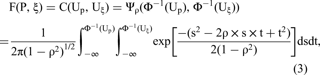
Let 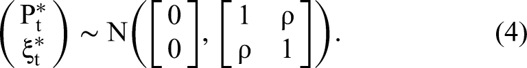


Next, we demonstrate that an implicit assumption for the previously generated regressor approach to yield consistent model estimates is the uncorrelatedness between
See the Web Appendix.
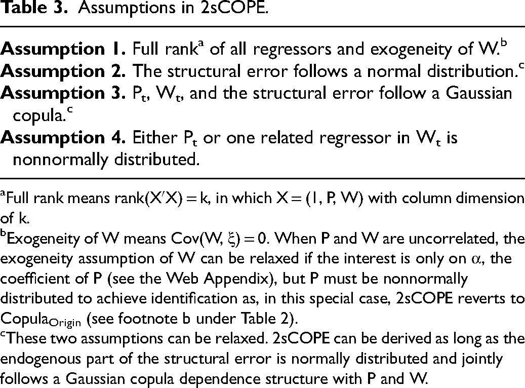
To summarize, CopulaOrigin based on Equation 6 makes the set of assumptions listed in Table 2. Assumption 5 has been discovered by Haschka (2022). However, as detailed in the Web Appendix, Assumption 5 should be replaced with the more general Assumption 5(b) for multiple endogenous regressors. 6 Assumptions 5 and 5(b) are verifiable and provide users with criteria to determine whether CopulaOrigin will provide consistent estimation when exogenous regressors exist. With only one endogenous regressor, one can simply check the correlations between the copula transformation of this endogenous regressor and each exogenous regressor. For multiple endogenous regressors, one should check the correlations between the CTT (i.e., the linear combination of copula transformations of these endogenous regressors used to control for endogeneity) in CopulaOrigin and each exogenous regressor, using Fisher's Z test, as described in the Web Appendix. Where Wt contains at least one exogenous regressor that fails Assumption 5 or 5(b), CopulaOrigin yields biased estimates, and our proposed 2sCOPE can be used, as derived in the next subsection.
Assumptions in CopulaOrigin.
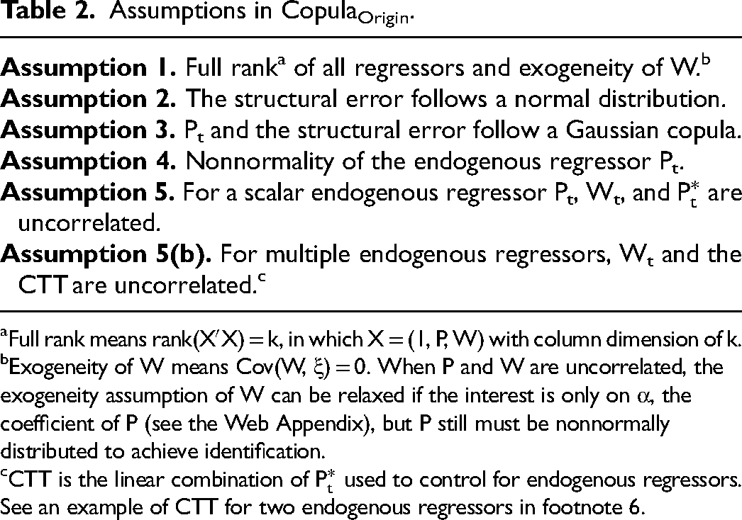
Full rank means rank(X′X) = k, in which X = (1, P, W) with column dimension of k.
Exogeneity of W means Cov(W, ξ) = 0. When P and W are uncorrelated, the exogeneity assumption of W can be relaxed if the interest is only on α, the coefficient of P (see the Web Appendix), but P still must be nonnormally distributed to achieve identification.
CTT is the linear combination of
The full rank of all regressors and exogeneity of Wt (Assumption 1 of Table 2) are assumptions that are made in several other commonly used econometric methods, including OLS and IV methods, to ensure estimation consistency. For Assumptions 2 to 4, Park and Gupta (2012) demonstrate their copula method's reasonable robustness to nonnormal distributions of the structural error (Assumption 2) and alternative forms of copula functions (Assumption 3), although it is not surprising to observe CopulaOrigin's sensitivity to gross violations of these assumptions, such as highly skewed error distributions (Becker, Proksch, and Ringle 2021; Eckert and Hohberger 2023). By contrast, the assumption that the endogenous regressor Pt follows a nonnormal distribution (Assumption 4) is critical. An endogenous regressor following a normal distribution violates the full-rank condition in Equation 6 and causes model unidentification regardless of the sample size; a nearly normally distributed endogenous regressor may require a very large sample size for the method to perform well and may cause the method to perform poorly for a finite sample size. Both Assumptions 4 and 5 (or 5(b)) can be too strong and substantially limit the copula method's applicability.
Proposed Two-Stage Copula Endogeneity-Correction Method
Here, we propose our 2sCOPE method and demonstrate its ability to relax both the uncorrelatedness assumption between CTT and the exogenous regressors (Assumption 5(b)) and the key identification assumption of nonnormal endogenous regressors (Assumption 4). The 2sCOPE method jointly models the endogenous regressor, Pt, the correlated exogenous variable, Wt, and the structural error term, ξt, using the Gaussian copula model, which implies that 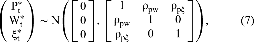
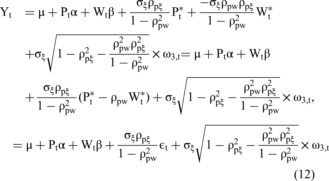
Under the Gaussian copula model in Equation 7, one may develop a direct extension of CopulaOrigin that adds the generated regressors
Under the Gaussian copula model in Equation 7, we have the following system of equations:

The main idea of 2sCOPE is to make use of the fact that, by conditioning on εt, the structural error ξt becomes independent of both Pt and Wt. That is, by conditioning on the component of Pt that causes its endogeneity (here, εt), the structural error is not correlated with either Pt or Wt, thereby ensuring the consistency of standard estimation methods. In this sense, εt serves as a (scaled) control function to address the endogeneity bias. To demonstrate this point, we rewrite the Gaussian copula model in Equation 7 as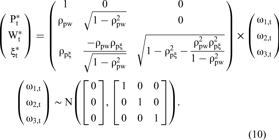

See the Web Appendix.
According to Theorem 2, the proposed method 2sCOPE can yield consistent estimates when assumptions are met. Specifically, Assumptions 5 and 5(b) are relaxed because 2sCOPE can handle the case in which the model includes exogenous regressors correlated with the CTT. Theorem 3 further demonstrates that 2sCOPE relaxes Assumption 4 (the nonnormality assumption on endogenous regressors), a critical model identification condition required in all other copula correction methods.
See the Web Appendix.
Theorem 3 shows that as long as one exogenous regressor correlated with the endogenous regressor Pt is nonnormally distributed, 2sCOPE can correct for endogeneity for a normal regressor Pt while COPE cannot. Intuitively, when Pt (or Wt) is normal,
Table 3 summarizes the assumptions used in the proof of the properties of 2sCOPE. Among these assumptions, Assumption 4 and the full rank of the regressor matrix in Assumption 1 are required and verifiable. We highlight the remaining assumptions that may be difficult to verify given that they involve the unobserved error term. W's exogeneity is required when P and W are correlated, and this assumption should be evaluated based on institutional knowledge or economic theory. Although Assumptions 2 and 3 are used in the proof, they are not strictly needed. Our simulation study demonstrates that 2sCOPE is robust to a range of nonnormal error distributions and reasonable departures from the Gaussian copula dependence model (see the Web Appendix). Furthermore, it is often reasonable to assume that the error term ξ may be expressed as ξ = U + V, where the normally distributed U stands for the joint effect of confounders (a linear combination of confounders) and V represents an independent disturbance term. When U and regressors jointly follow the Gaussian copula model, 2sCOPE corrects endogeneity bias. The assumption that U and regressors follow a Gaussian copula dependence model appears plausible given that the Gaussian copula is a widely used dependence model and is deemed sufficiently flexible to adequately capture multivariate dependence in many practical applications (Danaher and Smith 2011; Eckert and Hohberger 2023). Meanwhile, we emphasize that the Gaussian copula assumption warrants attention from those who employ copula methods.
Assumptions in 2sCOPE.
Full rank means rank(X′X) = k, in which X = (1, P, W) with column dimension of k.
Exogeneity of W means Cov(W, ξ) = 0. When P and W are uncorrelated, the exogeneity assumption of W can be relaxed if the interest is only on α, the coefficient of P (see the Web Appendix), but P must be nonnormally distributed to achieve identification as, in this special case, 2sCOPE reverts to CopulaOrigin (see footnote b under Table 2).
These two assumptions can be relaxed. 2sCOPE can be derived as long as the endogenous part of the structural error is normally distributed and jointly follows a Gaussian copula dependence structure with P and W.
In sum, we have demonstrated the consistency of 2sCOPE (Theorem 2). Theorem 3 and Proposition 1 (see the Web Appendix) further establish that 2sCOPE outperforms COPE, the extended CopulaOrigin, with respect to estimation efficiency and relaxation of the nonnormality assumption on endogenous regressors in CopulaOrigin by satisfying a looser condition.
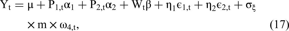
Multiple Endogenous Regressors
Herein, we extend 2sCOPE to the general case of multiple endogenous regressors. Consider the following structural linear regression model with two endogenous regressors (P1,t and P2,t) that are potentially correlated with the exogenous regressor Wt:


The Web Appendix presents the proof for the estimation consistency, relaxation of the regressor-nonnormality assumption, and estimation efficiency gain for 2sCOPE with multiple endogenous regressors under the related Theorems 2 and 3 and Proposition 1. Table 4 summarizes the estimation procedure of 2sCOPE.
Estimation Procedure for 2sCOPE.
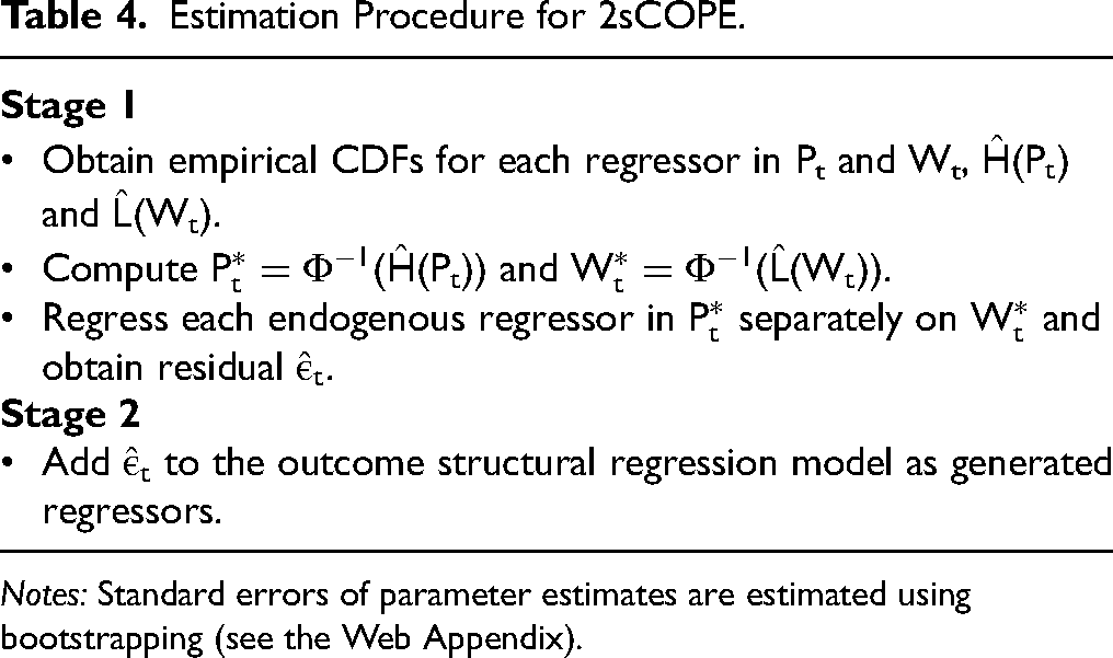
Notes: Standard errors of parameter estimates are estimated using bootstrapping (see the Web Appendix).
2sCOPE for Random Coefficient Linear Panel Models
We consider the following random coefficient model for linear panel data:
The linear panel data model as specified in Equation 18 is general and includes the linear panel model with only the individual-specific intercepts considered by Haschka (2022) as a special case. Specifically, Haschka fixes (αi, βi) to be the same value (α, β) across all units, assuming that all cross-sectional units have the same slope coefficients. By contrast, the model in Equation 18 relaxes this strong assumption and can generate unit-specific slope parameters that may be used for targeting purposes.
A random coefficient model typically assumes that (μi, αi, βi) follows a multivariate normal distribution. When all regressors are exogenous, estimation algorithms for such random coefficient models are well established and computationally feasible, even for a high-dimensional vector of random effects (μi, αi, βi). With the normal conditional distribution for Yit | (μi, αi, βi) in Equation 18 and the multivariate normal prior distribution for random effects (μi, αi, βi), Yit marginally follows a normal distribution with a closed-form expression that contains no integrals with respect to random effects (μi, αi, βi), leading to an easy-to-evaluate likelihood function (Wooldridge 2010). Alternatively, one may assume a mixed-effect model where μi is a fixed-effect parameter and can be correlated with the regressors Pit and Wit. In this case, the first-difference or fixed-effects transformation is typically used to eliminate the incidental intercept parameters as follows:
It is straightforward to apply 2sCOPE to address regressor endogeneity in the general random coefficient model for linear panel data in Equation 18 and the transformed model without intercepts in Equation 19.
7
The 2sCOPE procedure adds the residuals obtained from regressing
2sCOPE for Slope Endogeneity and Random Coefficient Logit Model
In the Web Appendix, we derive 2sCOPE to tackle slope endogeneity and address endogeneity bias in random coefficient logit models with correlated and normally distributed regressors. Unlike the MLE approach, 2sCOPE can be implemented using standard estimation methods through the addition of generated regressors to control for endogeneity.
Simulation Study
Here, we conduct Monte Carlo studies to assess (1) the proposed method's performance for correlated regressors, (2) the proposed method's performance under regressor normality and near normality, (3) the proposed method's performance under various types of structural models, and (4) the proposed method's robustness to violations of model assumptions. We measure the estimation bias using tbias calculated as the ratio of the absolute difference between the mean of the sampling distribution and the true parameter value to the standard error of the parameter estimate (Park and Gupta 2012). Thus, tbias represents the size of bias relative to the sampling error.
Case 1: Nonnormal Regressors
In the first case, P and W are correlated. The data-generating process (DGP) is summarized as follows: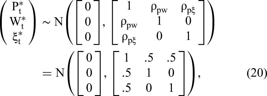

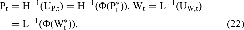
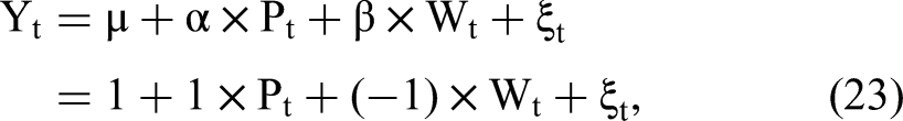
Table 5 reports estimation results. As expected, OLS estimates of both α and β are biased (tbias = 15.75 and 8.24) due to the regressor endogeneity. CopulaOrigin reduces the bias, but still shows significant bias for the coefficient estimates of Pt and Wt. The bias of CopulaOrigin depends on the strength of the correlation between W and P. Stronger correlations between P* and W* may cause the CopulaOrigin estimates to show a larger bias. For example, when the correlation between W* and P* increases from .5 to .7, the mean α estimate changes from 1.055 to 1.260 (see the CopulaOrigin column in Table 5), and, consequently, the bias of estimated α increases by around five times (from .055 to .260). The bias confirms our derivation in the model section, demonstrating that using the existing copula method may not wholly resolve the endogeneity problem with correlated regressors.
Results of Simulation Study Case 1: Nonnormal Regressors.
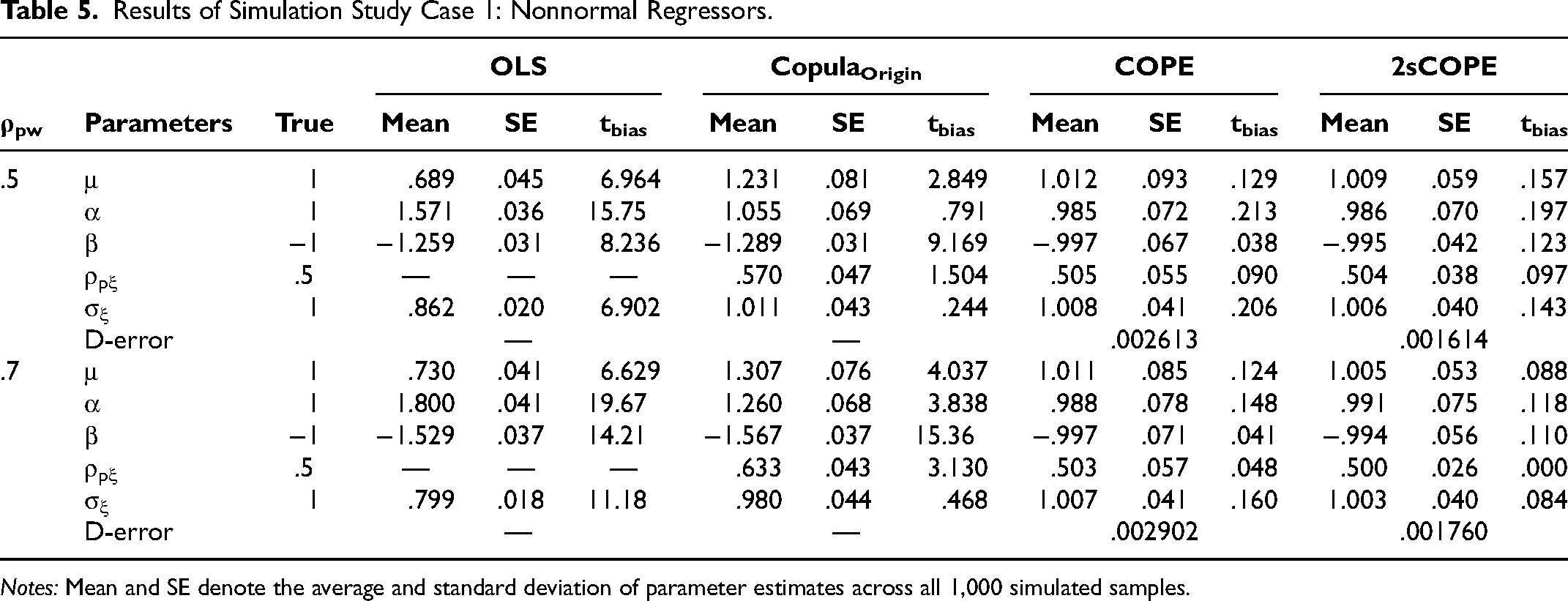
Notes: Mean and SE denote the average and standard deviation of parameter estimates across all 1,000 simulated samples.
The proposed 2sCOPE method provides consistent estimates without using instruments. The average estimate of ρpξ is close to the true value of .5 and differs significantly from 0, implying regressor endogeneity detected correctly using 2sCOPE. Moreover, 2sCOPE shows greater estimation efficiency. The standard error of α (β) in 2sCOPE is .070 (.042), which is 2.78% (37.31%) smaller than the corresponding standard errors using COPE. We further calculate COPE's and 2sCOPE's estimation precision using the D-error measure |Σ|1/K (Arora and Huber 2001; Qian and Xie 2022), where Σ is the covariance matrix of the regression coefficient estimates and K is the number of explanatory variables in the structural model. A smaller D-error indicates greater estimation efficiency and improved estimation precision. When ρpw = .5, the D-error measure is .002613 for COPE and .001614 for 2sCOPE (Table 5). Thus, 2sCOPE increases estimation precision by 38.2%, meaning that for 2sCOPE to achieve the same precision as COPE, the sample size can be reduced by 38.2%. A 39.3% efficiency gain for 2sCOPE is observed for ρpw = .7 (Table 5).
We perform a further simulation study for a small sample size using the same DGP as that described previously but with sample size T = 200. The results presented in Web Appendix Table W1 demonstrate that OLS estimates have endogeneity bias and CopulaOrigin reduces the endogeneity bias, but significant bias remains nonetheless. The proposed 2sCOPE performs well, yielding unbiased estimates for the small sample size T = 200. The efficiency gain of 2sCOPE relative to COPE appears to be greater for a smaller sample size. For example, when the correlation between P* and W* is .5, the D-error measures are .0166 and .0091 for COPE and 2sCOPE (Web Appendix Table W1), respectively, meaning that 2sCOPE increases estimation precision by 1 − .0091/.0166 = 46% compared with COPE. Thus, sample size can be reduced by almost half (∼50%) for 2sCOPE to achieve the same estimation precision as that achieved by COPE.
Case 2: Normal Regressors
Next, we examine a case in which the endogenous regressor and/or the correlated exogenous regressor are normally distributed. This case is of particular interest given that normality is not allowed for endogenous regressors in Park and Gupta (2012). We use the same DGP as that described in Equations 20 to 23, with the exception that the marginal CDFs for regressors, H(·) and L(·), are selected based on the distributions listed in the first two columns of Table 6, which summarizes the estimation results. As expected, the OLS estimates are biased. CopulaOrigin produces biased estimates whenever the endogenous regressor P follows a normal distribution. Its estimates are also biased when P follows a gamma distribution (first row of Table 6) for a different reason: P and W are correlated. Similar to CopulaOrigin, the COPE estimators in all three scenarios are biased when either Pt or Wt is normal. When Wt is normal, β is .323 away from the true value −1; when Pt is normally distributed, α is .684 away from the true value; when both Pt and Wt are normal, α is .663 away from the true value 1 and β is .324 away from the true value −1. This is expected because COPE adds
Results of Simulation Study Case 2: Normal Regressors.
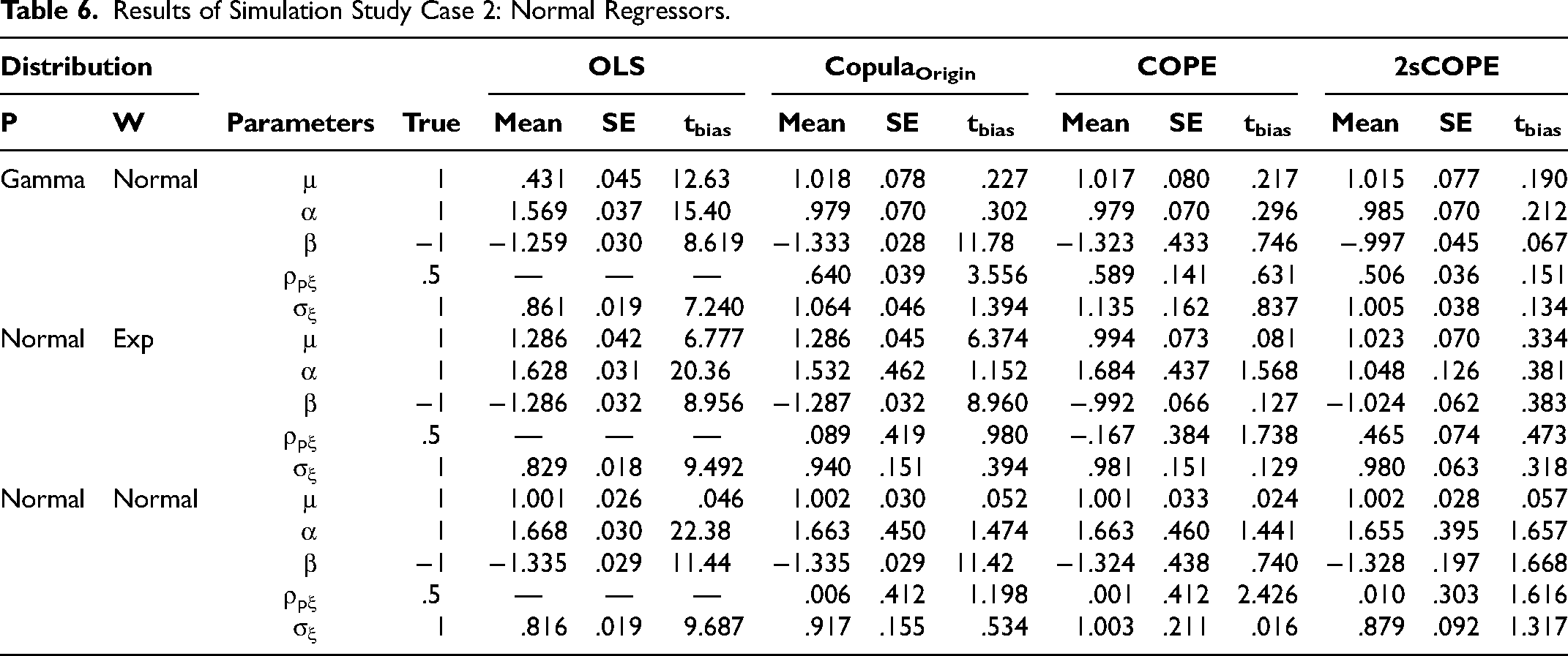
By contrast, the proposed 2sCOPE method provides consistent estimates as long as Pt and Wt are not both normally distributed. Both α and β are tightly distributed near the true value whenever Pt or Wt is nonnormally distributed. Unlike CopulaOrigin and COPE, 2sCOPE adds the residual term obtained from regressing
Case 3: Insufficient Nonnormality of Endogenous Regressors
The preceding case illustrates the proposed 2sCOPE's capability to deal with normal endogenous regressors while CopulaOrigin and COPE cannot. Here, we examine the more frequent scenario of close-to-normal regressors. Although models are identified asymptotically (i.e., infinite sample size), appreciable finite-sample bias may occur with the realistic sample sizes commonly seen in marketing studies, if the endogenous regressor is too close to a normal distribution (Becker, Proksch, and Ringle 2021; Eckert and Hohberger 2023; Haschka 2022). Becker, Proksch, and Ringle (2021) suggest a minimum absolute skewness of 2 for an endogenous regressor for CopulaOrigin to have good performance in sample sizes less than 1,000. This requirement can significantly limit the use of copula correction methods in practical applications. Given that 2sCOPE can handle normal endogenous regressors, we expect that 2sCOPE will be better able to handle the finite-sample bias caused by insufficient regressor nonnormality than the existing copula correction methods. We use the DGP described in Equations 20 to 23 to generate data, with the exception that the marginal CDF for the endogenous regressor (H(·)) varies across some common distributions with varying closeness to normality. Specifically, we consider uniform, lognormal, t, mixture normal, gamma, beta, and normal distributions, and use the average absolute estimation bias of all the regression parameters (μ, α, β) in the structural model to measure the performance.
Figure 1 plots the estimation bias with different distributions of the endogenous regressor P. The results reveal that the CopulaOrigin estimates are biased with correlated endogenous and exogenous regressors, consistent with our theoretical proof (Theorem 1). COPE performs well when P has sufficient nonnormality (t(2), lognormal, gamma) and exhibits no bias even for a sample size as small as 200. However, COPE cannot handle a normal endogenous regressor and yields a large estimation bias that remains unchanged as the sample size increases, consistent with our theoretical proof in Theorem 3 (see the Web Appendix) and the simulation result in Case 2. Furthermore, COPE suffers from finite-sample bias when the endogenous regressor P has distributions with insufficient nonnormality (e.g., beta(2,2), t(df = 30)). Moreover, COPE's estimation bias is larger when the sample size is smaller or the distribution of the endogenous regressor P is closer to normal. For instance, t distribution with 30 degrees of freedom is closer to normal than the t distribution with 10, 5, and 2 degrees of freedom, yielding a larger estimation bias. For t(df = 30), which is very close to normal, increasing the sample size from T = 200 to 1,000 scarcely changes the size of the estimation bias. By contrast, our proposed 2sCOPE method yields consistent estimates for all normal and close-to-normal regressor distributions and has negligible finite-sample bias even for a sample size as small as 200 (bias < 5% of parameter values).
Case 4: Random Coefficient Linear Panel Model
We investigate the performance of 2sCOPE in the random coefficient linear panel model. We use the copula function and marginal distributions of [Pit, Wit, ξit] as specified in Case 1 (Equations 20–22). We assign ρpw = .7 as an example. We then generate the outcome Yit using the following standard random coefficient linear panel model: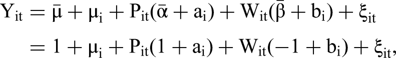
Results of Simulation Study Case 4: Random Coefficient Linear Panel Model.
Notes: σμ, σα, and σβ are standard deviations of μi, ai, and bi.
Additional Simulation Results and Robustness Checks
The Web Appendix provides additional simulation results on a small sample size; model estimation with multiple endogenous regressors; estimation with multiple exogenous control covariates including binary and close-to-normal control covariates; 2sCOPE's robustness to misspecifications of the structural error distribution and to misspecifications of the copula dependence structure; a test of Assumption 5(b); experimental studies to obtain practical recommendations for using 2sCOPE; the performance of 2sCOPE with one “strongly nonnormal” exogenous regressor versus multiple “weakly nonnormal” exogenous regressors for handling an endogenous regressor with insufficient nonnormality; the random coefficient logit model using 2sCOPE; 2sCOPE's performance when W is endogenous; and 2sCOPE's ability to leverage the empirical correlation between P and W. Overall, these results verify that 2sCOPE is robust to small sample sizes and reasonable violations of normal error and Gaussian copula assumptions, show that it is flexible to leverage control covariates and handle nonlinear models for choice outcomes, and provide guidance for 2sCOPE's use to obtain good performance, as summarized in the next section. Interestingly, the results reported in the Web Appendix indicate that a “strongly nonnormal” W is considerably more effective than multiple “weakly nonnormal” Ws in helping the identification of the causal effect for an endogenous regressor with insufficient nonnormality.
Guidelines for Using 2sCOPE
To summarize, we have established theoretical results that guarantee 2sCOPE's desirable large sample properties where correlated exogenous regressors exist (Theorem 2) and endogenous regressors have nonnormal distributions (Theorem 3). As expected, simulation studies demonstrate that 2sCOPE performs well when the sample size is sufficiently large. Meanwhile, simulation studies also reveal that, for 2sCOPE to perform well in finite samples, it may require sufficient regressor nonnormality and relevance between P and W (e.g., Figure 1, Panel A). To provide actionable guidelines for 2sCOPE's application to the data at hand, we conduct systematic simulation studies to establish the boundary conditions for using 2sCOPE. Specifically, the studies employ a factorial experimental design, which systematically varies the distributions of P and W, sample sizes, the level of endogeneity, and the strength of correlation between P and W. We evaluate 2sCOPE's performance using structural model parameter estimates’ relative bias. The Web Appendix provides details of the experimental design and results.
Figure 2 presents the decision tree for 2sCOPE's use based on the findings of the simulation studies. The decision tree comprises three steps. In Step 1, we test Assumption 5 (or 5(b) for multiple endogenous regressors) to choose between 2sCOPE and CopulaOrigin. When Assumption 5 (or 5(b)) is satisfied, CopulaOrigin is preferred over 2sCOPE because, although both methods provide consistent estimates, CopulaOrigin is more efficient (see the Web Appendix). Becker, Proksch, and Ringle (2021) provide a flowchart for the use of CopulaOrigin. Violation of Assumption 5 (or 5(b)) suggests the presence of relevant exogenous regressors that 2sCOPE may leverage to better handle endogeneity. In Step 2, we test the nonnormality of the endogenous regressor P using the Kolmogorov–Smirnov (KS) test (see the Web Appendix for the rationale of using the test of normality). If the KS test rejects the null at the .05 level, 9 P possesses sufficient nonnormality, and 2sCOPE has a high probability of success in correcting endogeneity bias based on the results detailed in the Web Appendix. Otherwise, P has a close-to-normal distribution, which requires related exogenous regressors with sufficient nonnormality and relevance to help identification. Thus, in Step 3, we check W's nonnormality and relevance to P. Results in the Web Appendix show that if the p-value of the KS test of an exogenous regressor W is smaller than .001 (i.e., sufficient nonnormality of W) and the relevance is sufficient (F-statistic for the effect of W* on P* > 10 in the first-stage regression), 2sCOPE will have a high probability of success.
We have provided sufficient conditions of endogenous and exogenous regressors in Steps 2 and 3 for 2sCOPE to have good finite-sample performance. These conditions are not necessary but are conservative. In particular, we consider extreme cases in which either the exogenous regressor in Step 2 or the endogenous regressor in Step 3 follows the normal distribution. In practice, regressors are more likely to have close-to-normal than exact normal distributions. The failure of W's sufficient condition tests does not necessarily preclude the use of 2sCOPE. For example, the estimation result of Scenario 1 in Web Appendix Table W12 (P and W are close-to-normal and weakly nonnormal, respectively) demonstrates that 2sCOPE may still show acceptable finite-sample performance when the preceding (conservative) sufficient conditions are not satisfied. In this scenario (the rightmost branch in Figure 2), one can employ our proposed bootstrap resampling Algorithm 1 to evaluate 2sCOPE's finite-sample performance on a case-by-case basis.
Simulate
Obtain
Obtain
Obtain the 2sCOPE estimate
Calculate potential bias of the 2sCOPE estimator:
Bootstrap simulations can be used to evaluate the bias size in parameter estimates when sample size is small to moderate (Efron and Tibshirani 1994, chap. 10; Hooker and Mentch 2018), 10 even if the estimation performs well for large samples. Specifically, Algorithm 1 randomly draws the same number of observations from the underlying copula model and the structural model estimated using the original sample, 11 and then performs the 2sCOPE estimation on the bootstrap sample as in the original sample. We repeat this simulation B times and obtain a distribution for each model coefficient estimate. We then compare the mean of each coefficient estimate's distribution with the corresponding coefficient estimate using the original data, which is the true parameter value in our model-based bootstrap resampling. The small-sample bias of a coefficient estimate is the difference between the average coefficient estimate from bootstrap samples and the original sample's coefficient estimate.
Empirical Application
In this section, we illustrate the proposed method to address the price endogeneity issue using store-level toothpaste category sales data for Chicago over 373 weeks from 1989 to 1997.
12
To control for product size, we select the most common weight, which is 6.4 oz. Specifically, we estimate the following sales model:
The correlation between log retail price and bonus promotion in Store 1 (Store 2) is −.31 (−.17), and the correlation between log retail price and price reduction promotion in Store 1 (Store 2) is −.22 (−.31). The appreciable correlations between price and promotion variables provide a suitable context for testing our method with correlated endogenous and exogenous regressors. The moderate sample size (T = 373) also allows us to evaluate 2sCOPE's finite-sample performance in the presence of potentially insufficient regressor nonnormality in real data. Table 8 reports summary statistics of the key variables.
Summary Statistics.
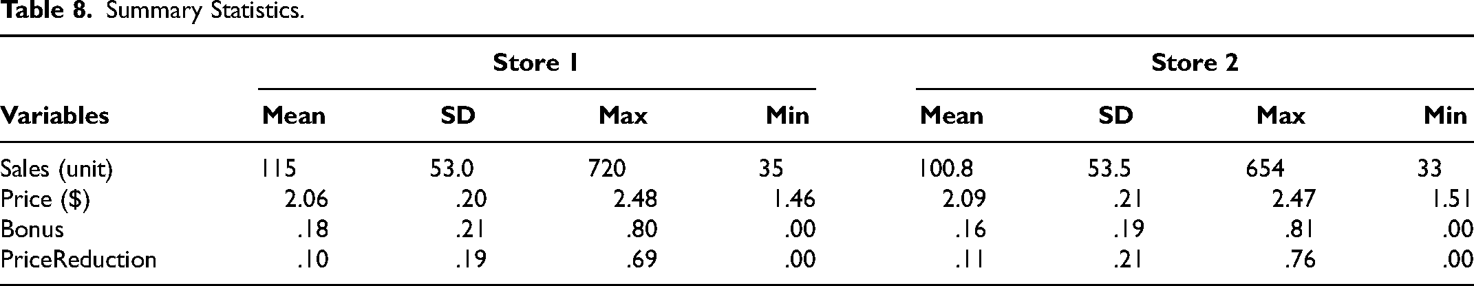
Figure 3 plots the log sales and log retail prices of toothpaste at Store 1 over time (Store 2 is very similar). To control for the possible time trend of retail price, we use detrended log retail prices (and detrended log values for IVs as well) for estimation. Figure 4 shows the histograms of detrended log retail prices and the two promotion variables. All three are continuous variables.
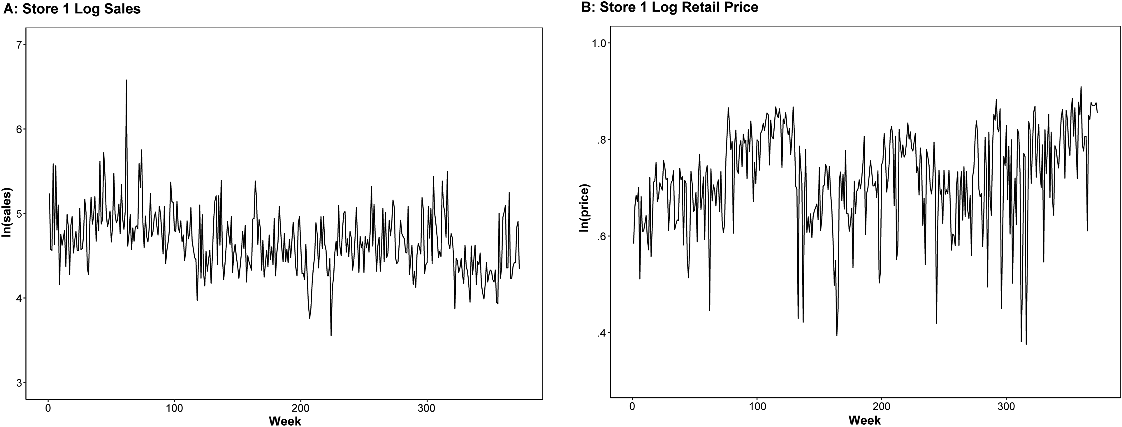
Log Sales and Log Retail Price of Toothpaste in Store 1.
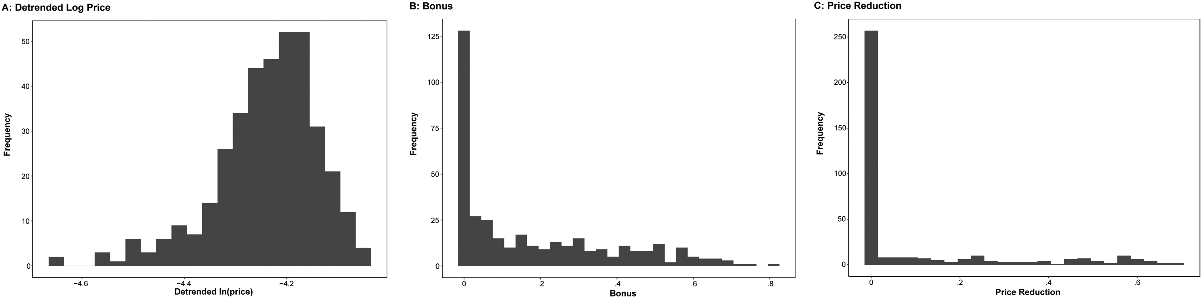
Histograms of Log Retail Price, Bonus, and Price Reduction in Store 1.
The flowchart in Figure 2 guides our use of 2sCOPE. In Store 1, the correlations between logP* and the exogenous regressors are −.44 for bonus promotion and −.27 for price reduction promotion, both of which differ substantially from zero with p-value < 2.2 × e−16 and 7.542 × e−08 respectively, indicating a violation of Assumption 5, which CopulaOrigin requires to yield consistent estimates. Next, we check the endogenous regressor's sufficient nonnormality. The KS test of the endogenous price yields a p-value of .063 > .05, indicating insufficient nonnormality of the endogenous price that CopulaOrigin (or COPE) cannot handle. We then proceed to check the exogenous regressors’ nonnormality and their relevance with the endogenous regressor. The bonus variable is strongly nonnormal (p-value of KS test = 3.159 × e−12) and sufficiently relevant (F-statistic = 89.5 > 10). Price reduction is also strongly nonnormal (p-value of KS test < 2.2 × e−16) and is sufficiently relevant (F-statistic = 27.3 > 10). Thus, according to Figure 2, the Store 1 dataset is appropriate for using 2sCOPE to correct endogeneity, and 2sCOPE is expected to have a high probability to achieve good finite-sample performance.
We next go through the flowchart for Store 2. First, the correlations between logP* and the exogenous regressors are −.32 for bonus promotion and −.39 for price reduction promotion, both of which are substantially different from zero with p-value 1.47 × e−10 and 5.32 × e−15 respectively, indicating a violation of Assumption 5 required for CopulaOrigin to yield consistent estimates. Next, we check the nonnormality of the endogenous regressor. The KS test of the endogenous price yields a p-value of .0053 < .05, indicating sufficient nonnormality of the endogenous price. Thus, according to the decision tree in Figure 2, the Store 2 dataset is also appropriate for using 2sCOPE to correct endogeneity. 14
We use the IV-based two-stage least squares (TSLS) estimator to cross-validate 2sCOPE's performance and the IV used. We use retail price at the other store as an instrument for price, which is commonly used in the literature (Park and Gupta 2012; Rossi 2014). This variable can be a valid instrument as it satisfies the two key requirements. First, retail prices across stores in a market can be highly correlated because wholesale prices are typically the same (or very similar). The Pearson correlation between the detrended log retail prices in Stores 1 and 2 is .76, providing strong explanatory power on the endogenous price. The correlation is comparable to that in Park and Gupta (2012). Second, unmeasured product characteristics such as shelf-space allocation, shelf location, and category location are determined by retailers and are usually not systematically related to wholesale prices (exclusion restriction). Meanwhile, unobserved national advertisement is not expected to affect production cost and wholesale price on a weekly basis and is thus expected to exert only a small effect on the variance of weekly wholesale price. Given that national advertisement occurs only in a few instances in any given planning time horizon (e.g., a quarter or a year), one would expect these demand shocks to be highly correlated and have a small variance over time at the weekly frequency (Rossi 2014). These considerations suggest that the exclusion restriction condition is reasonably satisfied in the presence of unobserved national advertisement. However, like other IVs, the validity claim cannot be fully verified, and is debatable. We therefore perform both 2sCOPE and TSLS so they can cross-validate each other. Congruent results from the two methods increase our confidence in endogeneity correction. Like TSLS, 2sCOPE includes (and uses) the existing exogenous regressors in the first-stage regression; however, unlike TSLS, 2sCOPE neither includes nor needs IVs. We first regress
Table 9 reports the estimation results. The OLS estimates in Store 1 differ significantly from TSLS estimates, suggesting the price endogeneity issue. Instrumenting for retail price changes the price coefficient estimate from −.767 to −1.797, implying a positive correlation between unobserved product characteristics and price. The 2sCOPE estimate of ρ, representing the correlation between the endogenous regressor Pt and the error term, is .297 (t-value = 3.34) and significantly positive, further confirming our conclusion and consistent with previous empirical findings (e.g., Chintagunta, Dubé, and Goh 2005; Villas-Boas and Winer 1999).
Estimation Results: Toothpaste Sales.
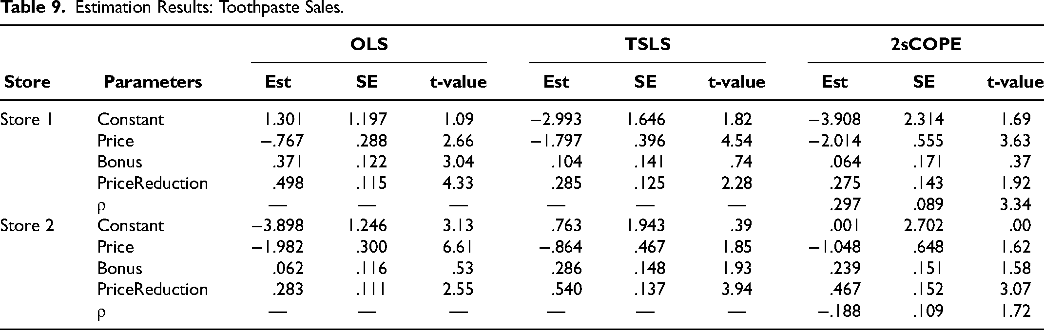
This positive price–error correlation causes upward bias (i.e., less price sensitivity) in the OLS price estimate. By directly accounting for this price–error dependence and controlling the first-stage residual, which captures unobserved product characteristics causing the positive correlation between the endogenous price and the error term, 2sCOPE corrects the classic upward endogeneity bias of price elasticity from −.767 to −2.014. The 2sCOPE price elasticity estimate of −2.014 is close to that of −1.797 from the TSLS method. Both 2sCOPE and TSLS price estimates show greater price sensitivity, suggesting that both correct the price endogeneity problem in the right direction. The TSLS and 2sCOPE estimates are reasonable because the price elasticity of the toothpaste category is approximately −2.0 (Chen and Lim 2022; Hoch et al. 1995; Mackiewicz and Falkowski 2015).
Unlike Store 1, Store 2's results indicate that the retail price is not endogenous. The estimate of ρ (the correlation between price and the error term) does not differ significantly from 0 for 2sCOPE (t-value ≤ 1.96 in the 2sCOPE column for Store 2 in Table 9). The OLS price estimate is −1.982, which is very close to the estimates of TSLS and 2sCOPE in Store 1, suggesting Store 2's lack of price endogeneity. Overall, the price elasticity estimates from TSLS and 2sCOPE are close for Store 2, and the observed differences between them and the OLS estimate may be attributed to the estimation variability incurred from the use of more complicated models compared with the OLS model.
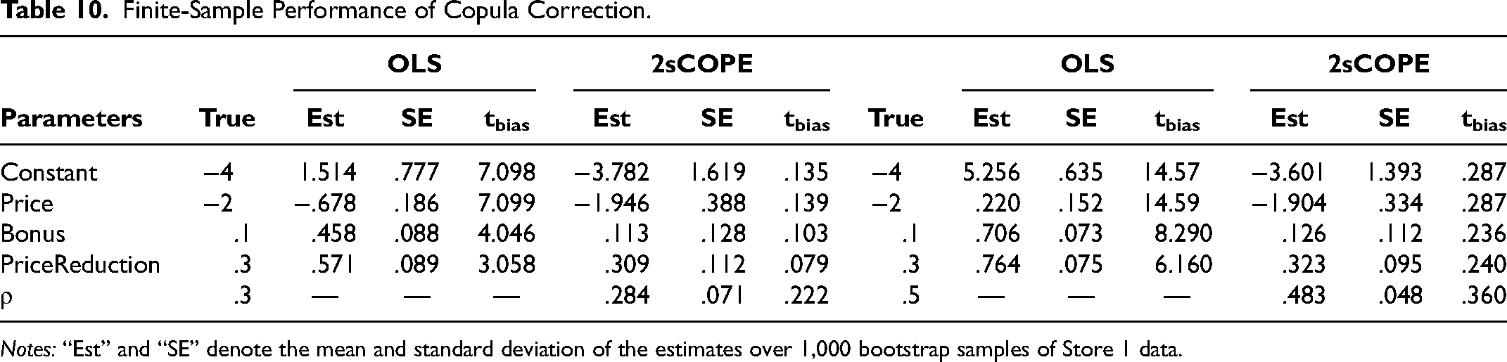
In the preceding application, the convergence of results between TSLS and the proposed 2sCOPE method in both stores supports the validity of the proposed method in addressing the endogeneity issue. The flowchart in Figure 2 also suggests our empirical data satisfy the boundary conditions under which 2sCOPE is expected to have good finite-sample performance. Although here it is unnecessary to empirically evaluate the finite-sample performance using the bootstrap resampling in Algorithm 1, we apply the algorithm to illustrate its usage in the empirical application. Specifically, we apply the bootstrap algorithm (Algorithm 1) to our empirical application with the true parameter values set as Store 1's 2sCOPE estimates (Table 9) rounded to the first nonzero number when generating bootstrap samples. We also consider the case in which ρ is set at .5, somewhat larger than the estimated value of ρ (.3), to assess the robustness of the bootstrap findings. The steps used to generate these bootstrap samples are detailed in the Web Appendix.
Table 10 summarizes the means and standard deviations of parameter estimates for OLS and 2sCOPE over the 1,000 bootstrap samples, unlike the estimation result on a single observed dataset reported in Table 9. The estimation results are broadly consistent with those in Table 9. In both cases (ρ = .3 and .5), the estimates of 2sCOPE are distributed closely to the true values, demonstrating that 2sCOPE corrects the bias of OLS estimates and performs well with little finite-sample bias in our empirical application.
Finite-Sample Performance of Copula Correction.
Notes: “Est” and “SE” denote the mean and standard deviation of the estimates over 1,000 bootstrap samples of Store 1 data.
Conclusion
Observational studies often require rigorous study designs and methodologies to overcome endogeneity concerns. While it is preferable to bring exogeneity via good instruments for identification, this is not always possible. In this article, we focus on the IV-free copula method to handle endogenous regressors, proposing our generalized 2sCOPE method that extends the existing copula correction methods (Becker, Proksch, and Ringle 2021; Eckert and Hohberger 2023; Haschka 2022; Park and Gupta 2012) to more general settings. Specifically, 2sCOPE permits the correlation of exogenous regressors with endogenous regressors and relaxes the nonnormality assumption on the endogenous regressors. Similar to CopulaOrigin, 2sCOPE corrects endogeneity by adding “generated regressors” derived from existing regressors and is straightforward to use. However, unlike CopulaOrigin, which adds the latent copula transformations of endogenous regressors directly to the model, 2sCOPE has two stages. The first obtains the residuals from regressing latent copula data for the endogenous regressor on the latent copula data for the exogenous regressors, while the second uses the first-stage residual as a “generated regressor” in the structural regression model. We prove that 2sCOPE yields consistent causal effect estimates when the normally distributed structural error and all regressors follow a Gaussian copula correlation structure. The 2sCOPE method can also relax the nonnormality assumption on endogenous regressors and substantially improve copula correction's finite-sample performance.
We evaluate 2sCOPE's performance via simulation studies and demonstrate its use in an empirical application. The simulation results show that 2sCOPE yields consistent estimates under relaxed assumptions. Moreover, 2sCOPE outperforms CopulaOrigin (and COPE) in terms of dealing with close-to-normal or normal endogenous regressors and improving estimation efficiency. Endogenous regressors are allowed to have close-to-normal or even normal distributions with the help of exogenous regressors (Figure 2). The efficiency gain relative to COPE is substantial and may reach ∼80% in simulation studies (see the Web Appendix), implying that 2sCOPE can reduce by ∼80% the sample size needed to achieve the same estimation efficiency as COPE, which does not exploit the correlations between endogenous and exogenous regressors. Finally, robustness checks indicate that 2sCOPE is reasonably robust to the structural error distributional assumption and non-Gaussian copula correlation structure (see the Web Appendix). We further apply 2sCOPE to a public dataset in marketing. Regarding endogenous price, we find that the estimated price coefficient using our proposed 2sCOPE is very close to the TSLS estimate and the price coefficient reported in the literature, while the OLS estimator indicates substantial biases.
These findings have rich implications regarding the practical use of the copula-based IV-free methods for handling endogeneity. A known critical assumption for CopulaOrigin is the nonnormality of endogenous regressors. The users of the method have largely checked and verified this assumption. However, our findings indicate that this is insufficient: it is also necessary to check Assumption 5 for the single endogenous regressor case and Assumption 5(b) for the case of multiple endogenous regressors. Neither assumption is the same as checking the pairwise correlations between the endogenous and exogenous regressors. Assumption 5 evaluates pairwise correlations involving copula transformation of the endogenous regressor, which, as shown in the literature (Danaher and Smith 2011) and in our specific empirical application, may differ substantially from the pairwise correlations using the original variables. Assumption 5(b) evaluates the correlations between exogenous regressors and the linear combination of generated regressors, which differ even more considerably from pairwise correlations on the regressors themselves. We expect that Assumptions 5 and 5(b) will be violated in the majority of practical applications (see the result of real-data application in footnote 15 and the Web Appendix), for which 2sCOPE should be used. Even in exceptional cases that satisfy the preceding assumptions, 15 2sCOPE can still be used successfully (see the Web Appendix). Yet in these exceptional cases, CopulaOrigin may be considered (Figure 2, Step 1) since the simpler and valid model gains estimation/prediction efficiency and is easier to understand, use, and communicate with as a decision calculus tool (Little 2004).
For endogenous regressors with insufficient nonnormality or exogenous regressors that violate Assumptions 5 or 5(b), 2sCOPE outperforms CopulaOrigin and is recommended. When all endogenous regressors have sufficient nonnormality, 2sCOPE is expected to perform well. If any endogenous regressor has insufficient nonnormality, 2sCOPE exploits exogenous regressors with sufficient relevance and nonnormality levels (Figure 2 details sufficient conditions) for satisfactory model identification in finite samples. One can empirically check and verify whether these conditions are satisfied for data at hand, using normality and relevance tests. For cases in which these conditions are not met, we also propose a novel bootstrap resampling method (Algorithm 1) to directly gauge and validate 2sCOPE's finite-sample performance in real applications on a case-by-case basis, complementing the preceding rules of thumb using tests of normality and relevance. According to the decision-tree check using real-world data, 98% of cases result in using 2sCOPE in the decision tree (Figure 2), demonstrating the overwhelming need for 2sCOPE (Web Appendix Table W11).
Unlike the TSLS method, 2sCOPE requires no IVs that must satisfy the exclusion restriction condition. Exclusion restriction is considerably more stringent than the exogeneity condition in that the IV not only is exogenous but also does not appear in the outcome model, meaning that the IV cannot affect the outcome Y by any means other than the endogenous regressor. 16 It is typically impossible to test exclusion restriction; one must rely on institutional knowledge and theoretical arguments to establish exclusion restriction's credibility, which is often the most challenging aspect of IV applications. By contrast, our approach eliminates the requirement that any variable satisfy the exclusion restriction assumption, which constitutes a significant gain. Using 2sCOPE, one need not argue for exclusion restriction, but for the regressors and the error following a copula dependence structure.
Meanwhile, 2sCOPE is capable of leveraging relevant exogenous variables in W in the outcome model (e.g., in Equation 8) for model identification. Marketing models rarely contain endogenous regressors exclusively; the majority of the outcome models estimated (e.g., using OLS or IVs) in marketing include exogenous variables for various reasons, such as the inclusion of exogenous regressors as control variables to mitigate the endogeneity concern of the primary explanatory variables, to improve model estimation and forecasting accuracy, to make the outcome models substantively complete and relevant, or to render the exclusion restriction assumption of IVs more plausible. These exogenous control variables influence other variables in the marketing model but are determined outside the model and are unaffected by the model outcomes. Common examples include environmental factors (e.g., weather), macroeconomic indicators (e.g., interest rate, GDP growth, inflation rates), government policies and legal rules, natural disasters and events, customer characteristics used by firms for targeting, and marketing activities (e.g., promotions) prearranged on an annual basis and independent of daily/weekly demand shocks.
These exogenous regressors are not used to generate the copula control function in CopulaOrigin. By contrast, 2sCOPE can leverage these exogenous variables to improve model identification and estimation. Such exogenous control variables are much more widely available than the IVs because 2sCOPE does not require any of these exogenous variables to satisfy the stringent exclusion restriction condition. Furthermore, no theoretical arguments are required for the direction and intuition of correlation between W and P. An empirical correlation is sufficient (see the Web Appendix). 17 Finally, when endogenous regressors have insufficient nonnormality, 2sCOPE can leverage exogenous regressors with certain nonnormality and relevance levels (Figure 2), which are feasible in many applications, for identification.
To fully benefit from leveraging relevant control covariates in W for handling endogeneity, these control covariates need to be exogenous. In practice, choosing a good set of exogenous control variables requires care in model specification and may pose empirical challenges for data analysts. Similar to OLS, TSLS, and CopulaOrigin, the addition of endogenous variables to W can yield inconsistent model estimates for 2sCOPE. 18 Thus, certain types of variables that violate the exogeneity condition, such as mediators or colliders, should be excluded from W. For example, consumer perceptions of price levels and emotions toward stores are found to lie in the causal pathway between pricing and demand (Cakici and Tekeli 2022). Such mediators are endogenous (affected by the endogenous pricing variable), and, consequently, including them (e.g., measured using periodic consumer surveys) in W and treating them as being exogenous when estimating a demand model will introduce overcontrol bias (Hernan and Robins 2023). Additionally, if these mediators are also influenced by the unobserved determinants of the sales outcome (e.g., store service quality), then the two mediators could also be colliders influenced by both the primary explanatory variables and the outcome. Including colliders in the regression and treating them as exogenous control variables is known to cause collider bias (Hernan and Robins 2023). The remedy is to exclude mediators and colliders from W. Like other econometric methods, the reasonableness of the exogenous W assumption should be evaluated and justified in the context of the objectives and scopes of analysis. In this respect, substantive or institutional knowledge is useful for guiding or justifying the selection of appropriate exogenous control covariates. To avoid violating the exogeneity assumption about W, we recommend practicing clean adjustment employing only exogenous control variables necessary to improve causal effect estimation. Control variables strongly believed to be endogenous should be treated as endogenous regressors in the model or removed from the model. 19 In this respect, 2sCOPE can offer ways of tackling some major challenges encountered in model specifications: For example, certain control variables must be included to mitigate endogeneity concerns in OLS estimation or make the exclusion restriction assumption of IVs plausible but are nonetheless believed to be endogenous and thus pose a dilemma as to whether they should be included in the model for the OLS or TSLS estimation.
Although 2sCOPE contributes to solving regressor endogeneity by relaxing key assumptions of the existing copula correction methods and extending them to more general settings, it is not without its limitations. For 2sCOPE to function optimally, the endogenous regressors’ distributions must contain adequate information. The condition is violated when the endogenous regressors follow Bernoulli distributions or discrete distributions with small support, as Park and Gupta (2012) note. The proposed 2sCOPE method does not address this limitation. The simplicity of 2sCOPE assumes the normal structural error and Gaussian copula dependence structure. Our evaluation demonstrates that 2sCOPE is robust to symmetric nonnormal error distributions, linear dependence among endogenous and exogenous regressors, and certain non-Gaussian copula structures (see the Web Appendix). Such robustness may not hold for highly skewed error distributions or other forms of dependence or copula structure. Future research is needed to test and relax these assumptions using more flexible copula methods. Despite these limitations, we expect that 2sCOPE will provide a useful alternative to a broad range of empirical problems when instruments are unavailable. Although our empirical application only considered linear sales models, potential empirical applications of 2sCOPE abound. We have derived 2sCOPE and evaluated its performance via simulated data for a range of other commonly used marketing models, including linear panel models with mixed effects, random coefficient logit models, and slope endogeneity. Future empirical studies may apply 2sCOPE to these and many other cases not studied here.
Supplemental Material
sj-pdf-1-mrj-10.1177_00222437241296453 - Supplemental material for Addressing Endogeneity Using a Two-Stage Copula Generated Regressor Approach
Supplemental material, sj-pdf-1-mrj-10.1177_00222437241296453 for Addressing Endogeneity Using a Two-Stage Copula Generated Regressor Approach by Fan Yang, Yi Qian and Hui Xie in Journal of Marketing Research
Footnotes
Acknowledgments
The authors are very grateful to the JMR review team and seminar and conference participants for many constructive comments that have significantly improved the article. All inferences, opinions, and conclusions drawn in this study are those of the authors, and do not reflect the opinions or policies of the funding agencies and data stewards. No personal identifying information was made available as part of this study. Procedures used were in compliance with British Columbia's Freedom in Information and Privacy Protection Act. Ethics approval was obtained from the University of British Columbia's Behavioral Research Ethics Board (H15-00887).
Coeditor
Raghuram Iyengar
Associate Editor
Marnik Dekimpe
Declaration of Conflicting Interests
The author(s) declared no potential conflicts of interest with respect to the research, authorship, and/or publication of this article.
Funding
The author(s) disclosed receipt of the following financial support for the research, authorship, and/or publication of this article: This work was supported by the Social Sciences and Humanities Research Council of Canada (grants 435-2018-0519 and 435-2023-0306), Natural Sciences and Engineering Research Council of Canada (grants RGPIN-2018-04313 and RGPIN-2024-06629), U.S. National Institutes of Health (grant R01CA178061), and AoE research fund from NEOMA Business School, France (grant 416006).
Notes
References
Supplementary Material
Please find the following supplemental material available below.
For Open Access articles published under a Creative Commons License, all supplemental material carries the same license as the article it is associated with.
For non-Open Access articles published, all supplemental material carries a non-exclusive license, and permission requests for re-use of supplemental material or any part of supplemental material shall be sent directly to the copyright owner as specified in the copyright notice associated with the article.