Detecting Routines: Applications to Ridesharing Customer Relationship Management

Abstract

Routines shape many aspects of day-to-day consumption. While prior research has established the importance of habits in consumer behavior, little work has been done to understand the implications of routines—which the authors define as repeated behaviors with recurring, temporal structures—for customer management. One reason for this dearth is the difficulty of measuring routines from transaction data, particularly when routines vary substantially across customers. The authors propose a new approach for doing so, which they apply in the context of ridesharing. They model customer-level routines with Bayesian nonparametric Gaussian processes, leveraging a novel kernel that allows for flexible yet precise estimation of routines. These Gaussian processes are nested in inhomogeneous Poisson processes of usage, allowing the authors to estimate customers’ routines and decompose their usage into routine and nonroutine parts. They show the value of detecting routines for customer relationship management in the context of ridesharing, where they find that routines are associated with higher future usage and activity rates, and more resilience to service failures. Moreover, the authors show how these outcomes vary by the types of routines customers have, and by whether trips are part of the customer's routine, suggesting a role for routines in segmentation and targeting.

Routines are an integral feature of consumers’ daily lives: for many people, from the time they wake up to the moment they go to sleep, their time is structured around routines. Such routines often involve consumption, like picking up coffee from a favorite coffee chain each morning, checking a weather app before going outside, or choosing a mode of transportation to get to and from work. Moreover, consumers’ routines differ from one another: while one person may drink their coffee only in the mornings, seven days per week, another may prefer to have their coffee after lunch, and only on weekdays. Marketers can greatly benefit from understanding consumer routines. Yet, while routines are intuitively important drivers of consumer behavior, prior research has not explored the presence of such routines in consumers’ behavior and their implications for customer management. Accordingly, the objectives of this research are (1) to build a statistical model that can capture customer routines at the individual level and (2) to explore the relationship between such routines and behavioral outcomes like transaction frequency and customer activity.

We define a routine as a behavior with a defined, recurring, temporal structure, such that the same behavior occurs at roughly the same time, period after period. We focus specifically on the period of a week, as weekly routines capture many common routines, including, for instance, weekday commutes, weekday lunches, weekend brunches, and weekly grocery shopping. ¹ Routines are related to habits, which have been studied more extensively in marketing (e.g., Drolet and Wood 2017). It is the emphasis on temporal structure that differentiates routine behavior from habitual (or repeat) behavior. For example, a consumer who always shops at the same store may do so out of habit. A customer who always shops at that same store every Thursday evening exhibits a routine. In this sense, a routine can be viewed as a habit that is embedded in a consumer's day-to-day schedule. We posit that such temporally structured behavior may be an especially important predictor of customer value, and customer behavior more generally.

Little research has been done on capturing routines and understanding their impact on consumer behavior and firm profitability. In this work, we focus on the implications of routines for customer relationship management (CRM). In particular, we hypothesize that, given equal transaction rates, customers who interact with the company as part of their routine may be higher-value customers, in terms of more future purchasing and lower rates of churn, relative to customers with no routine. Routine customers may also be better customers in other ways, including having lower price sensitivities and higher resilience to service disruptions. We hypothesize that the effect of a routine exists over and above a mere tendency to repurchase the same product, as is already captured in many existing CRM frameworks like the recency–frequency–monetary value (RFM) model (e.g., Blattberg, Neslin, and Kim 2008; Neslin et al. 2013). In other words, given two customers with identical purchasing summary statistics—that is, they both purchased recently, they both made the same number of purchases historically, and they both spent the same amount on each purchase occasion—we predict that the customer whose purchase timings exhibited a higher routineness will be a better customer in the future.

To measure customer routineness, we develop a statistical model that allows us to identify the routine of each individual customer, if it exists, and isolate the share of the consumption that can be attributed to that routine. This model enables us to differentiate between, for instance, a customer who has ten routine trips per week (e.g., to and from work every weekday) and another customer who has only two routine trips per week (e.g., going to yoga class on Tuesday and Thursday afternoons). Specifically, our model is an individual-level, inhomogeneous Poisson process that captures individual-specific patterns in consumption across periods, with a unique Bayesian nonparametric specification of its rate. The individual-specific rate of consumption is decomposed into a component that captures potentially dynamic levels of idiosyncratic or “random” consumption, and a “routine” component that captures individual-level consistencies in consumption timing, which is modeled using a Gaussian process (GP) prior with a unique kernel structure. This kernel structure incorporates intuitive aspects of consumption over time—specifically, that certain days exhibit similarities in consumption (e.g., a Tuesday might be more similar to a Thursday than to a Sunday) and that consumption within days exhibits a 24-hour cycle (e.g., 12:05 a.m. is similar to 11:55 p.m.)—to precisely estimate individual-specific variation in routine behavior. Using the routine component of the Poisson rate parameter, we construct an individual-specific “routineness” metric that measures the degree to which an individual's behavior is structured around a routine. In addition to the routineness metric, the model infers the form or temporal “shape” of the routine for each consumer (e.g., whether a consumer has a Monday through Thursday morning routine or a Tuesday evening routine).

We apply our model and routineness metric to data from Via, a leading New York City–based ridesharing company, to estimate consumer routines in requesting rides. Ridesharing is a particularly rich setting for studying routines, as travel is often an integral part of many daily and weekly routines. We identify various patterns in using the ridesharing service across users, including predictable commuting routines as well as more complex, idiosyncratic routines. More importantly, we show that, as hypothesized, users who are more routine in their behavior are also more valuable to the firm, in terms of both higher future usage and higher rates of remaining active, even after controlling for past usage patterns such as recency, frequency, or clumpiness. Having established the value of routineness in customer value, we then show that routines also play a role in driving and moderating other aspects of the customer–firm relationship, including price sensitivity and customer response to service failures. Our results suggest that firms can benefit from understanding routines for better predicting future customer activity and developing segmentation and targeting strategies. Notably, routines moderate customer behavior both between customers, insofar as more routine customers behave differently than less routine customers, and within customers, insofar as customers react differently to pricing and service for trips that are part of their routines. The between-customer effects suggest that the firm may benefit from identifying routine users, or even cultivating routines, while the within-customer effects suggest that there is room for firms to optimize the provision of services around customers’ routines.

The rest of the article is organized as follows. We start by discussing the prior literature on habits and routines and the connections between routineness and other extant metrics of transaction timing in CRM. We then present our model for capturing and measuring customer-specific routines. Moving next to our empirical application, we describe the ridesharing data and the results of applying our model: We first apply the model on synthetic data that mimics the real data, validating the model's ability to recover different types of routines. We then apply the model on the ridesharing data, characterizing the types of routines exhibited by riders, and validating the model's fit. Finally, we explore the idea of routineness more deeply by highlighting the relevance of routines for CRM, exploring how customer-level outcomes vary by the type of routine, and comparing routineness with other constructs. We conclude with discussion and directions for future research.

Conceptual Foundations

While research on routines is relatively scant, the closely related topics of habits and repeat behaviors have been studied extensively, both in marketing and in related disciplines. Early work in marketing used the term “repeat buying habit” to indicate the practice of repeatedly buying the same product or repeatedly buying from the same company, without considering the more psychological construct of a habit or habit formation (Ehrenberg and Goodhardt 1968). Predicting repeat purchasing has subsequently been the focus of many models in customer base analysis, including popular buy-till-you-die models (e.g., Schmittlein, Morrison, and Colombo 1987) and more general RFM-based specifications (e.g., Dew and Ansari 2018). Repeat buying is also central to other important marketing constructs, including brand and store loyalty and brand inertia (e.g., Guadagni and Little 1983), all of which can also be viewed as forms of habitual behavior. Moving beyond studying simple repeat purchasing, Shah, Kumar, and Kim (2014) generalized the idea of habits to recurring behaviors like returning products, purchasing on promotion, and purchasing low-margin items. They showed that these repeat behaviors are linked to firm profitability, and that firm actions can influence the formation of habitual behaviors.

Habit formation has also been studied in economics, often in the context of consumption and expenditure, where it is typically defined as current expenditures depending on lagged expenditures through a “habit stock.” In this literature, habits have been used to explain the smoothness of consumption over time, even in the presence of shocks to income, although evidence for the existence of habit formation in aggregate consumption is mixed (Dynan 2000; Fuhrer 2000).

Much of the theory behind why habits matter, how they develop, and how they can be changed has come from the psychology and consumer behavior literatures. Habits have been studied in psychology since as early as the nineteenth century (James 1890). In this literature, habits are often defined as tendencies to repeat behaviors, typically automatically or subconsciously (Ouellette and Wood 1998; Wood, Quinn, and Kashy 2002), and sometimes in a goal-directed manner (Aarts and Dijksterhuis 2000) or triggered by contextual cues (Neal et al. 2012). Especially relevant for our empirical application of ridesharing, habits have recently been identified as a primary driver of travel mode choice (e.g., Verplanken et al. 2008), which is of particular interest for developing more sustainable consumer choices (White, Habib, and Hardisty 2019). A noteworthy finding in this literature is the habit discontinuity hypothesis, which states that context changes that disrupt individuals’ habits can lead to deliberate choice consideration and habit breaking (Verplanken et al. 2008). This phenomenon has also been observed in the CRM literature. For example, Ascarza, Iyengar, and Schleicher (2016) show that customers who continue to transact with the firm out of habit may be driven to churn by company retention efforts, even when those retention efforts are intended to save the customer money, simply by means of disrupting their inertia.

Routines and Habits

In one sense, routines can be viewed as a specific type of habit, where the automaticity of behavior is related to time: if, every day, at a certain time, a consumer carries out an action, then time can be considered the context that triggers that behavior. Thus, many of the predictions made elsewhere in the literature about habitual behavior and customer loyalty (e.g., Ascarza et al. 2018) carry over to routines: we postulate, for instance, that routines can lead to nearly automatic choices, and will thus be more difficult to break, resulting in stickier long-term behavior and lower likelihood to react negatively to price increases or service failures. However, we hypothesize that routines are more predictive of customer value than mere habit. The key distinction between habits and routines is that whereas habits simply imply automatic, repeated behaviors, a behavior is routine only if it additionally has a recurring, temporal structure. Intuitively, such behaviors are likely embedded in a consumer's daily life and, thus, may be even more automatic and indicative of long-term value than habitual behaviors that lack such a temporal structure. Thus, a customer who is routinely consuming a focal product or service may be even more valuable than one who is merely habitually (i.e., repeatedly) consuming the product, but not in a routine manner.

Clumpiness, Regularity, and Routines

Our work is also related to the growing literature on extending traditional RFM frameworks to incorporate information about usage and purchase timing. RFM-based frameworks, while useful predictive tools, discard much of the richness of a customer's transaction history and simply summarize a customer's likelihood of repeat purchasing by how recently they purchased and how often they purchased in the past. Recent work has shown that there is incremental value in moving beyond these simple statistics. A notable contribution in this stream is Zhang, Bradlow, and Small (2015), who defined the “clumpiness” of customer transaction times. Their metric captures the customer-level entropy of intervisit times and is higher when a customer exhibits more temporally clustered, or “clumpy,” behavior. They show that, in many empirical contexts, especially contexts with bingeable content, this measure of clumpiness is a key (positive) predictor of customer lifetime value. Another key contribution comes from Platzer and Reutterer (2016), who defined the concept of transaction regularity. In particular, they introduced a buy-till-you-die model, the Pareto/GGG, where the regularity of transactions is modeled by relaxing the standard exponential-distributed intertransaction time model common to many customer base models, allowing for customer-specific gamma-distributed intertransaction times. They find that incorporating regularity can improve customer-level predictions.

Routineness is conceptually distinct from, but related to, these two metrics. In particular, routines can generate clumpy or regular behavior, or even regular clumpy behavior, depending on the type of routine. For example, a customer who takes multiple rides club-hopping every Saturday night exhibits a routine that is clumpy, while a “workaholic” customer who takes a ride to work seven days a week exhibits very regular behavior. We illustrate these ideas in Figure 1. In contrast, a customer who commutes only on Mondays and Wednesdays may have a routine that is neither clumpy nor regular. In other words, the measures are distinct: not all routines are clumpy or regular, and not all clumpy or regular behaviors are routine. ²

Figure 1.

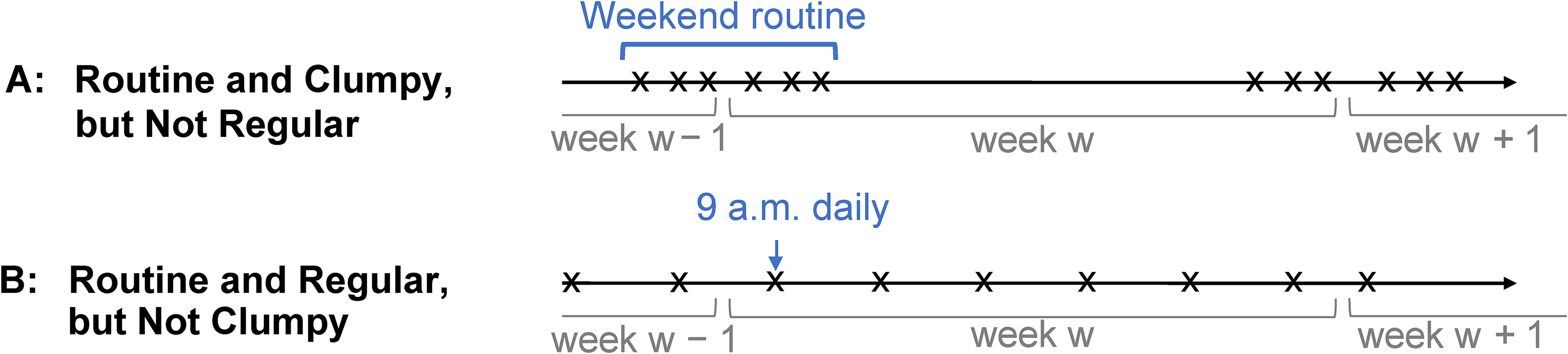
Clumpy and Regular Routines.

That routines can generate clumpy and regular behavior is a key advantage of our framework for several reasons. First, routines add additional nuance to the possible “types” of clumpiness that can be observed, thereby partly answering a call from Kumar and Srinivasan (2015) to explain the origins of clumpiness in transactions. Relatedly, this link between routines, clumpiness, and regularity also sheds light on when clumpy and regular transaction times, which intuitively seem at odds, may both be predictive of higher customer value, insofar as both may be manifestations of routines. More broadly, the interpretability of routines makes routineness a valuable metric for marketers looking to build interpretable yet accurate CRM models, thus addressing an ongoing need for new advances in this space (Neslin et al. 2006). Finally, our novel approach of identifying and isolating routines using transaction data and relating them to the customer value is consistent with Du et al.’s (2021) call to move toward a richer characterization of behavior and toward relating such behaviors to firm growth through customer value.

Model

In this section, we specify a model of usage that yields a natural metric for how routine a customer's behavior is, and what weekly routine the customer exhibits. By “usage,” we mean the consumer interacting with the firm in some way, and by “weekly routine,” we mean the structure of usage within a given week, which is the main focus of this research. Before describing the model, we first review its methodological underpinnings.

Methodological Background

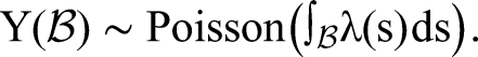
The model we propose merges an inhomogeneous Poisson process with a Bayesian nonparametric Gaussian process (GP). While the basis of many customer base analysis models is a homogeneous Poisson process (Schmittlein, Morrison, and Colombo 1987), inhomogeneous Poisson process transaction models have been employed to capture more complex dynamics in usage or transaction behavior (e.g., Ascarza and Hardie 2013; Ho, Park, and Zhou 2006). An inhomogeneous Poisson process is a point process over some space, $\mathcal{S}$ , where the rate of observing events, λ(s), depends on position in the space, $\mathrm{s}\in \mathcal{S}$ , such that the number of events in any bounded region of the space, $\mathrm{Y}(\mathcal{B}),\mathcal{B}\subseteq \mathcal{S}$ , is distributed:

$$\mathrm{Y}(\mathcal{B})\sim \mathrm{Poisson}\left({\int }_{\mathcal{B}}\lambda (\mathrm{s})\mathrm{ds}\right).$$

In many marketing applications, the space $\mathcal{S}$ is time (i.e., $\mathcal{S}=\mathbb{R}$ ), such that the process simply captures that events are not uniformly likely over time. Poisson processes have several useful properties, including the superposition property, which says that if Y₁ and Y₂ are Poisson processes with rates λ₁ and λ₂, then Y₁ + Y₂ is also a Poisson process with rate λ₁ + λ₂ (Kingman 1992). We make use of this property in our model specification to separate routine from nonroutine transactions.

In our model, the time-varying rate parameter of the Poisson process is modeled using a GP (Williams and Rasmussen 2006). In marketing, GPs have seen increased use in recent years, in both aggregate-level and individual-level CRM and brand choice contexts (Dew and Ansari 2018; Dew, Ansari, and Li 2020; Tian and Feinberg 2021). Regarding our research objective, GPs offer an ideal solution to modeling routines because, unlike other flexible function estimation methods, they enable us to flexibly model customer-level rates of usage while also allowing us to encode prior knowledge about the structure of time. We elaborate on this point in the following subsection. In the broader literature, our model aims to capture time-varying purchasing or usage patterns and is thus related to a long line of dynamic models in marketing (e.g., Du and Kamakura 2012; Kim, Menzefricke, and Feinberg 2005).

Model Specification

We propose a model of customer usage of a focal product or service. The key dependent variable, denoted y_it, captures how many times customer i interacts with the company during time period t. When we apply this model to ridesharing data, the dependent variable will be requesting rides. However, our model is fully general and can be applied using timing data from any context, at various time intervals, and for myriad customer behaviors of interest (e.g., using a mobile app, making purchases with the firm, visiting the firm's website).

We model a customer's observed usage y_it as the amalgamation of two individual-level, inhomogeneous Poisson processes over time (t): a routine process ${\mathrm{y}}_{\mathrm{i}}^{\mathrm{Routine}}(\mathrm{t})$ , which captures how often consumption needs arrive as part of the customer's routine, and a nonroutine or “random” process, ${\mathrm{y}}_{\mathrm{i}}^{\mathrm{Random}}(\mathrm{t})$ , which captures how often consumption needs arrive outside of the customer's routine. Throughout the article, we use the words “nonroutine” and “random” interchangeably. The idea is that usage outside of the routine is likely due to random needs arising, from the point of view of the customer, not that this process is totally random (i.e., white noise). Each of these processes has its own customer-specific rate, ${\lambda }_{\mathrm{i}}^{\mathrm{Routine}}(\mathrm{t})$ and ${\lambda }_{\mathrm{i}}^{\mathrm{Random}}(\mathrm{t})$ . As the analyst, we do not observe whether a given transaction is routine or not; we only observe the collection of all transactions, ${\mathrm{y}}_{\mathrm{i}}(\mathrm{t})\equiv {\mathrm{y}}_{\mathrm{i}}^{\mathrm{Routine}}(\mathrm{t})+{\mathrm{y}}_{\mathrm{i}}^{\mathrm{Random}}(\mathrm{t})$ . This additivity assumption implies that usage in a customer's routine can increase or decrease independently of usage outside the routine, and vice versa. By the superposition property described previously, we have that y_i(t) is also a Poisson process, with rate given by ${\lambda }_{\mathrm{i}}^{\mathrm{Routine}}(\mathrm{t})+{\lambda }_{\mathrm{i}}^{\mathrm{Random}}(\mathrm{t})$ . Meaningfully decomposing overall usage into routine and nonroutine parts thus requires specifying these rates.

To specify these rates, we first simplify our setting by assuming that the analyst only cares about time on a discrete grid, such that we only consider the number of uses that occur within fixed intervals. Slightly abusing notation, we use t to refer to this fixed time grid. Given our intuition that routines are customer-level behaviors that are consistent in terms of when they occur, week over week, the relevant grid to consider consists of weeks (w), days within weeks (d), and hours within days (h), the collection of which gives us t = (w, d, h). We assume that w indexes weeks since the start of the data, d indexes days of the week starting with d = 1 = Sunday, and h = 0, …, 23 indexes the 24 hours of a day. To simplify notation even further, we use the unit of “day-hours,” which we denote as j = 1 + (d − 1) × 24 + h, such that j = 1, …, 168 captures all the hours in a week. Under this time structure, the dependent variable y_it = y_iwj captures the number of interactions customer i has with the firm in week w at day-hour j.

Under this discrete time assumption, our model likelihood can be specified as

$${\mathrm{y}}_{\mathrm{it}}\sim \mathrm{Poisson}({\lambda }_{\mathrm{it}}^{\mathrm{Routine}}+{\lambda }_{\mathrm{it}}^{\mathrm{Random}}),$$

(1)

where ${\lambda }_{\mathrm{it}}^{\mathrm{Routine}}={\int }_{\tau \in \mathrm{t}}{\lambda }_{\mathrm{i}}^{\mathrm{Routine}}(\tau )\mathrm{d}\tau$ , and likewise for ${\lambda }_{\mathrm{it}}^{\mathrm{Random}}$ . We denote the overall usage rate as ${\lambda }_{\mathrm{it}}\equiv {\lambda }_{\mathrm{it}}^{\mathrm{Routine}}+{\lambda }_{\mathrm{it}}^{\mathrm{Random}}$ . We then break each of the overall usage rate terms into two dynamic parameters:

$${\lambda }_{\mathrm{it}}=\exp ({\gamma }_{\mathrm{iw}}+{\eta }_{\mathrm{ij}})+\exp ({\alpha }_{\mathrm{iw}}+{\mu }_{\mathrm{j}}).$$

(2)

In each term, there is one parameter that varies over weeks (w) and one that varies over day-hours (j). Our substantive focus is primarily on variation over day-hours. Thus, noting that λ_it could be rewritten as ${\lambda }_{\mathrm{it}}=\exp ({\gamma }_{\mathrm{iw}})\exp ({\eta }_{\mathrm{ij}})+\exp ({\alpha }_{\mathrm{iw}})\exp ({\mu }_{\mathrm{j}})$ , we refer to the terms with j subscripts (i.e., η_ij and μ_j) as “day-hour rate” terms, reflecting the rate of usage across day-hours, and refer to the terms with w subscripts (i.e., γ_iw and α_iw) as “weekly scaling” terms, as these terms scale up or down each of the rate terms over customers and weeks. ³

We next explain how this structure maps onto the idea of routines as week-over-week consistencies in time of use. In the first term, the routine rate, ${\lambda }_{\mathrm{it}}^{\mathrm{Routine}}=\exp ({\gamma }_{\mathrm{iw}}+{\eta }_{\mathrm{ij}})$ , the day-hour rate parameter, η_ij, has an i subscript. Thus, η_ij captures patterns of day-hour usage that are specific to customer i. If the weekly scaling parameter, γ_iw, is large for many subsequent weeks, it suggests that the customer is expected to use the service consistently at the same day-hours each week, following the pattern determined by η_ij. However, in the second term, the nonroutine or “random” rate, ${\lambda }_{\mathrm{it}}^{\mathrm{Random}}=\exp ({\alpha }_{\mathrm{iw}}+{\mu }_{\mathrm{j}})$ , the day-hour rate parameter does not have an i subscript. Instead, this term captures general patterns of day-hour usage that are common across customers and across weeks. For example, in our empirical application, μ_j captures that, on average, customers tend to take rides during the day, but not in the middle of the night. Said differently, if any given user were to randomly have need of the service, μ_j captures when we might expect that random need to arise and how the distribution of random needs may deviate from a uniform distribution over day-hours. If this term's weekly scaling parameter, α_iw, is high, it suggests that the customer is expected to make many requests that week, but that the day-hour pattern of those requests is not consistent with that customer's week-over-week patterns. It is this tension between consistently using the service at the same (individual-specific) day-hours, versus using the service in a way that is “random” (up to the typical usage patterns in the population), that implicitly defines what our model detects as a routine: if the usage follows a customer-specific day-hour pattern that is consistent over weeks, over and above the general consistency implied by the customer base as a whole, that usage will be captured by the first term and is what our model defines as routine usage.

Recall that the superposition property implies that our model can be equivalently expressed as the sum of two count processes, ${\mathrm{y}}_{\mathrm{it}}={\mathrm{y}}_{\mathrm{it}}^{\mathrm{Routine}}+{\mathrm{y}}_{\mathrm{it}}^{\mathrm{Random}}$ , such that

$${\mathrm{y}}_{\mathrm{it}}^{\mathrm{Routine}}\sim \mathrm{Poisson}(\exp ({\gamma }_{\mathrm{iw}}+{\eta }_{\mathrm{ij}})),$$

(3)

$${\mathrm{y}}_{\mathrm{it}}^{\mathrm{Random}}\sim \mathrm{Poisson}(\exp ({\alpha }_{\mathrm{iw}}+{\mu }_{\mathrm{j}})).$$

(4)

This decomposition allows for a natural definition of the levels of random usage and routine usage through the expectation of Poisson random variables. Specifically, we define two metrics, ${\mathrm{E}}_{\mathrm{iw}}^{\mathrm{Routine}}$ and ${\mathrm{E}}_{\mathrm{iw}}^{\mathrm{Random}}$ , which are the expected number of random and routine interactions, respectively, within a single week w, for customer i, such that

$${\mathrm{E}}_{\mathrm{iw}}^{\mathrm{Routine}}=\sum _{\mathrm{j}}\exp ({\gamma }_{\mathrm{iw}}+{\eta }_{\mathrm{ij}}),$$

(5)

$${\mathrm{E}}_{\mathrm{iw}}^{\mathrm{Random}}=\sum _{\mathrm{j}}\exp ({\alpha }_{\mathrm{iw}}+{\mu }_{\mathrm{j}}).$$

(6)

In plain English, these two terms capture how often a user is expected to interact with the firm in a given week, decomposing the total number of interactions into the expected number of interactions happening at random, and the number of interactions stemming from the user's routine. These metrics allow us to identify how routine customers’ behaviors are, and they are at the heart of the article's focus and intended contribution. We call ${\mathrm{E}}_{\mathrm{iw}}^{\mathrm{Routine}}$ the routineness of customer i in week w, and we use this metric and terminology throughout our analysis.

Specifying the Components of the Usage Rates

Our model captures individual-level, time-varying usage through two count processes, each of which has a rate ( ${\lambda }_{\mathrm{it}}^{\mathrm{Routine}}$ and ${\lambda }_{\mathrm{it}}^{\mathrm{Random}}$ , respectively) that comprises two parts: scaling terms (α_iw and γ_iw) and day-hour rates (μ_j, and η_ij). To model these parameters, we first recast the problem as estimating latent functions α_i(w), γ_i(w), μ(j), and η_i(j), respectively. This switch from subscript notation to functional notation is merely a conceptual pivot: by recasting the problem of estimating rates as a problem of estimating unknown functions, we can capture uncertainty over those rates using GPs. As we show, this in turn allows us to encode prior knowledge and assumptions about these parts of the model in a natural way, beyond those that could be incorporated in other specifications (e.g., state space models). ⁴

GPs provide a way of specifying prior distributions over spaces of functions. With this prior, we can encode structural information about the functions in that space, like the smoothness and differentiability of the functions, or other a priori knowledge about their shape. In this way, GPs allow for flexible estimation of functions, while optimally leveraging both information sharing and a priori knowledge, to improve the efficiency of those estimates. A GP is a distribution over functions, $\mathrm{f}(\mathrm{x}):{\mathbb{R}}^{\mathrm{d}}\to \mathbb{R}$ , defined by two other functions: a mean function, m(x), which captures the a priori expected function value at inputs x, and a kernel function k(x, x′), which captures a priori how similar we expect the function values f(x) and f(x′) to be for two inputs x and x′. Modeling f(x) using a GP is denoted as f(x) ∼ GP(m(x), k(x, x′)). For a finite, fixed set of inputs, x = (x₁, …, x_N), f(x) ∼ GP(m(x), k(x, x′)) is equivalent to

$$\mathrm{f}({\mathrm{x}}_1,\dots ,{\mathrm{x}}_{\mathrm{N}})\sim \mathrm{N}(\mathrm{m}({\mathrm{x}}_1,\dots ,{\mathrm{x}}_{\mathrm{N}}),\mathrm{K}),$$

(7)

such that element (n₁, n₂) of K is given by ${\mathrm{K}}_{{\mathrm{n}}_1,{\mathrm{n}}_2}=\mathrm{k}({\mathrm{x}}_{{\mathrm{n}}_1},{\mathrm{x}}_{{\mathrm{n}}_2})$ . Mathematically, the matrix K is the kernel k(x, x′) evaluated pairwise over all inputs and is called the kernel matrix. Intuitively, a GP specifies a multivariate Gaussian prior over the outputs corresponding to any combination of inputs, by means of its mean function and kernel. Thus, these two objects are the primary source of model specification in GP-based models. In practice, it is common to set the mean function m(x) to be zero or a constant and let the dependencies between the outputs be solely captured by the kernel (Williams and Rasmussen 2006). The primary restriction in specifying the kernel is that the corresponding kernel matrix be positive definite. The mean function and kernel themselves are typically parameterized through an additional set of parameters referred to as hyperparameters.

Returning to our specification, we model the following:

$${\gamma }_{\mathrm{i}}(\mathrm{w})\sim \mathrm{GP}({\gamma }_{0\mathrm{i}},{\mathrm{k}}_{\mathrm{Exp}}(\mathrm{w},{\mathrm{w}}^{\mathrm{\prime }};{\varphi }_{\gamma })),$$

(8)

$${\alpha }_{\mathrm{i}}(\mathrm{w})\sim \mathrm{GP}({\alpha }_{0\mathrm{i}},{\mathrm{k}}_{\mathrm{Exp}}(\mathrm{w},{\mathrm{w}}^{\mathrm{\prime }};{\varphi }_{\alpha })),$$

(9)

$${\eta }_{\mathrm{i}}(\mathrm{j})\sim \mathrm{GP}(0,{\mathrm{k}}_{\mathrm{DH}}(\mathrm{j},{\mathrm{j}}^{\mathrm{\prime }};{\varphi }_{\eta })),$$

(10)

$$\mu (\mathrm{j})\sim \mathrm{GP}(0,{\mathrm{k}}_{\mathrm{DH}}(\mathrm{j},{\mathrm{j}}^{\mathrm{\prime }};{\varphi }_{\mu })).$$

(11)

Here, ${\mathrm{k}}_{\mathrm{Exp}}(\cdot ,\cdot )$ is the exponential kernel, and ${\mathrm{k}}_{\mathrm{DH}}(\cdot ,\cdot )$ is a novel day-hour kernel, both of which we define subsequently. In γ_i(w) and α_i(w), we allow for individual-level constant mean functions, γ_0i and α_0i, capturing the mean level of routine and nonroutine usage for each customer. The ϕs are kernel hyperparameters.

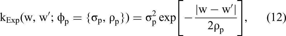
The kernel used for both of the weekly terms is the exponential kernel (e.g., Dew, Ansari, and Li 2020), given by the general form,

$${\mathrm{k}}_{\mathrm{Exp}}(\mathrm{w},{\mathrm{w}}^{\mathrm{\prime }};{\varphi }_{\mathrm{p}}=\{{\sigma }_{\mathrm{p}},{\rho }_{\mathrm{p}}\})={\sigma }_{\mathrm{p}}^2\exp \left[-{\displaystyle \frac{|\mathrm{w}-{\mathrm{w}}^{\mathrm{\prime }}|}{2{\rho }_{\mathrm{p}}}}\right],$$

(12)

where the p subscript corresponds to the hyperparameters of parameter p. For this kernel, p is either γ or α. ⁵ The exponential kernel is a special form of the more general Matérn kernel, a popular kernel often used to model functions that may exhibit smooth fluctuations over time (Dew, Ansari, and Li 2020; Williams and Rasmussen 2006). ⁶ The smoothness of the underlying process is captured by the kernel's length-scale parameter, ρ. The higher this parameter, the more covariance is expected between function values, given fixed inputs. We illustrate the effect of the length-scale parameter on smoothness of the function draws in Figure 2. In the context of routines, we expect that the routine weekly scaling parameter, γ_i(w), will be smoother than the nonroutine parameter, α_i(w). This additional smoothness mathematically corresponds to our intuition that a routine should be consistent week over week. We embed this a priori expectation by defining different priors for ρ_γ, the length scale of γ_i(w), and ρ_α, the length scale of α_i(w), as we discuss in the next section.

Figure 2.

Draws from a GP Prior.

The other kernel, ${\mathrm{k}}_{\mathrm{DH}}(\mathrm{j},{\mathrm{j}}^{\mathrm{\prime }};\varphi )$ , is a novel kernel that we term the “day-hour kernel.” This kernel has a functional form designed to capture the a priori structure we know exists within weeks, specifically that hours follow a 24-hour cycle and that certain days are more similar to other days (e.g., weekends vs. weekdays, workdays vs. days off). To capture these properties, we fuse a periodic kernel (Williams and Rasmussen 2006, Chapter 4) with an unstructured estimate of the correlation between different days of the week. Specifically, we define

$${\mathrm{k}}_{\mathrm{DH}}(\mathrm{j},{\mathrm{j}}^{\mathrm{\prime }};{\varphi }_{\mathrm{p}}=\{{\sigma }_{\mathrm{p}},{\rho }_{\mathrm{p}},{\mathrm{\Omega }}_{\mathrm{p}}\})={\sigma }_{\mathrm{p}}^2\times {\mathrm{\Omega }}_{\mathrm{p}}[\mathrm{d},{\mathrm{d}}^{\mathrm{\prime }}]\times \exp \left\{-{\displaystyle \frac{1}{2{\rho }_{\mathrm{p}}^2}{\sin }^2\left({\displaystyle \frac{\pi |\mathrm{h}-{\mathrm{h}}^{\mathrm{\prime }}|}{24}}\right)}\right\},$$

(13)

where, again, p indexes a particular parameter, which in this case, can be either μ or η. The matrix Ω_p is a correlation matrix over days of the week, and the notation Ω_p[d, d′] stands for the (d, d′) entry of that matrix (i.e., the correlation between days d and d′). This correlation matrix can be seen as an unstructured kernel that allows the model to detect, in a fully flexible way, the correlation structure that exists between function values across different days. The third term in this product is the periodic kernel with a 24-hour cycle, denoted ${\mathrm{k}}_{\mathrm{Per}}(\mathrm{h},{\mathrm{h}}^{\mathrm{\prime }};{\rho }_{\mathrm{p}})$ for short. It captures the smooth but cyclic variation we expect to see over hours within a day, with smoothness ρ_p. Thus, our day-hour kernel is a specific form of the more general class of multiplicative kernels, formed by specifying kernels separately on input dimensions (in this case, days and hours), then multiplying those kernels together. Crucially, for our day-hour kernel to be valid, the kernel matrix formed by evaluating our kernel pairwise at all input values must always be positive (semi)definite. The kernel matrix (for parameter p) implied by our DH kernel is given by

$${\mathrm{K}}_{\mathrm{DH}}={\sigma }_{\mathrm{p}}^2{\mathrm{\Omega }}_{\mathrm{p}}\otimes {\mathrm{K}}_{\mathrm{Pe}{\mathrm{r}}_{\mathrm{p}}},$$

(14)

where, analogous to previous kernel matrices, ${\mathrm{K}}_{\mathrm{Pe}{\mathrm{r}}_{\mathrm{p}}}$ is the matrix formed by evaluating the periodic kernel ${\mathrm{k}}_{\mathrm{Per}}(\mathrm{h},{\mathrm{h}}^{\mathrm{\prime }};{\rho }_{\mathrm{p}})$ pairwise at all hours. To see that this matrix is positive definite, first, note that we restrict Ω to be a correlation matrix, and thus, Ω is positive definite. K_Per is guaranteed to be positive definite, since ${\mathrm{k}}_{\mathrm{Per}}(\mathrm{h},{\mathrm{h}}^{\mathrm{\prime }};{\rho }_{\mathrm{p}})$ is known to be a valid kernel (Williams and Rasmussen 2006). Thus, since the Kronecker product of two positive definite matrices is also positive definite, we see that k_DH(j, j′) is a valid kernel.

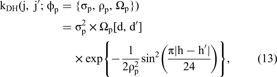
Intuitively, this day-hour kernel allows us to place a prior over functions that exhibit two natural properties when dealing with weekly usage data: we allow for arbitrary relatedness of days through the unstructured correlation matrix Ω_p, and for a natural 24-hour cycle through ${\mathrm{k}}_{\mathrm{Per}}(\mathrm{h},{\mathrm{h}}^{\mathrm{\prime }};{\rho }_{\mathrm{p}})$ , which accounts for the fact that usage at h = 0 (12 a.m.) will be similar to usage at h = 23 (11 p.m.). Finally, through its multiplicative structure, it assumes that these two forces operate together: if day d is similar to day d′, as captured by Ω_p, and hour h is similar to hour h′, a GP modeled with this kernel is expected to have similar function values at (d, h) and (d′, h′). By encoding this natural prior information into our model structure, we facilitate the efficient inference of the mean and individual-level rate functions, μ(j) and η_i(j).

Hyperparameter Priors

To complete our fully Bayesian specification, we briefly describe the priors for the hyperparameters of our GP kernels, the most important of which are the length-scale parameters, ρ_α and ρ_γ. Recall that these hyperparameters control the smoothness of the weekly scaling parameters, and that we expect, a priori, that ρ_γ will be larger than ρ_α. To encode that in our model, we draw on the suggestions by Betancourt (2020) and use weakly informative inverse-gamma priors. ⁷ The inverse-gamma distribution, given by

$$\mathrm{f}(\mathrm{x}\mid \mathrm{a},\mathrm{b})={\displaystyle \frac{{\beta }^{\mathrm{a}}}{\mathrm{\Gamma }(\mathrm{a})}{\mathrm{x}}^{-\mathrm{a}-1}\exp \left({\displaystyle \frac{-\beta }{\mathrm{x}}}\right),}$$

has a shape parameter a and a scale parameter β. For both ρ_α and ρ_γ, we set the shape parameter a = 5, which implies a 1% quantile of around 1. ⁸ The value of b is set differently for ρ_α and ρ_γ and may depend on the empirical application. In short, b can be thought of as scaling the inverse-gamma distribution, effectively changing the magnitude of the draws. Thus, higher values will allow for higher length scales, corresponding to higher smoothness. In our application, we set b = 5 for ρ_α and b = 11 for ρ_γ. ⁹ This setting encourages higher values for ρ_γ, corresponding to higher smoothness of γ_i(w) over weeks, which is exactly what our definition of routineness entails. Meanwhile, the relatively lower prior expectation for ρ_α does not enforce any a priori smoothness, which corresponds to allowing random needs to arise at any time. ¹⁰

To estimate the correlation matrix Ω in the day-hour kernel, we use a Lewandowski–Kurowicka–Joe (LKJ) prior for correlation matrices, such that Ω ∼ LKJ(2), which puts a weak prior toward the identity matrix (Lewandowski, Kurowicka, and Joe 2009). ¹¹ Intuitively this prior is setting a (weak) expectation that different days will not be related to each other, essentially imposing no prior assumptions about how strongly days will be related to one another, or which days will be related to each other. This flexibility is a key advantage of this approach over a parametric kernel. ¹²

Finally, for the individual-level constant mean functions, γ_0i and α_0i, we specify these in a hierarchical way, such that ${\gamma }_{\mathrm{i}0}\sim \mathrm{N}(0,{\sigma }_{{\gamma }_0})$ , and analogously for α_i0. For all other parameters, we use standard, weakly informative normal or half-normal priors. ¹³

Inference

We estimate the model parameters in a fully Bayesian fashion using the no-U-turn sampler (NUTS), a gradient-based Markov chain Monte Carlo sampler. To improve the scalability of the framework, we use the NUTS implemented in NumPyro and code our model in PyMC. This implementation of NUTS can be run on a graphics processing unit (GPU), which is significantly faster than central processing unit (CPU)-based implementations.

In its simplest form, our model can be computationally difficult: while discretizing the arrival times into hourly buckets makes defining the kernel and estimating the GPs easier (due to the limited number of inputs and natural structure between days, weeks, and hours), it also forces the model to do likelihood computations over many time periods in which nothing happened. That is, customers often interact with the firm sparsely, yet our likelihood function is specified as a count variable over all time periods t = (w, d, h), which forces us to consider all the zeroes. To help facilitate inference in this setup, we draw on a property of Poisson variables described in Gopalan, Hofman, and Blei (2015). Specifically, the log-likelihood of our model for all observations from a single customer i can be decomposed into two terms:

$$\log \mathrm{p}({\mathrm{y}}_{\mathrm{i}}|{\lambda }_{\mathrm{i}})=\sum _{{\mathrm{y}}_{\mathrm{it}}\ne 0}{\mathrm{y}}_{\mathrm{it}}\log ({\lambda }_{\mathrm{it}})-\sum _{\mathrm{t}}{\lambda }_{\mathrm{it}}+\mathrm{C},$$

(15)

where C is a constant with respect to λ_it. The first term in this expression depends only on the nonzero values of y_it, while the second term is a simple sum over all λ_it. In this way, the likelihood can operate only on the nonzero values of y_it, circumventing the potentially problematic sparsity.

Parameter Recovery, Model Scalability, and Data Applications

We conducted simulations to test the model's ability to recover the data-generating process and the model's performance under multiple different data settings. Specifically, we investigated three questions: (1) For data generated from the model (i.e., with known routines and stochastic transaction process), how well can the model's parameters be recovered? (2) How well does the model perform with varying degrees of data (i.e., number of customers, and number of time periods)? (3) How robust is the model's performance in the presence of customer churn? In this subsection, we briefly summarize the results and refer interested readers to Web Appendix B for more details.

Even with relatively little data (e.g., 100 customers over 20 weeks), the model can recover the data-generating process: correlations between true and estimated (posterior median) parameters ranged from .96 for population parameters (like μ(j)) to .74 for individual-level parameters (like η_i(j)). ¹⁴ More importantly, if we look at the estimated number of routine and random requests, the correlation between simulated and estimated values is as high as .98. These results hold in the presence of churn, although model performance is best when churn rates are low, in which case churn is relatively rare, or fairly high, in which case most customers churn during the calibration period.

Model Extensions

The framework we have introduced is quite general and only requires the analyst to have access to transactional data. In some cases, we may wish to incorporate covariates in the model specification to understand how other events, like firm interventions, or past service quality may relate to routine and random usage. Such covariates can be included by expanding the rate specification in Equation 2 to include covariate effects. We give an example of such an extension and describe the potential complexities that emerge when trying to meaningfully incorporate covariates in our model in Web Appendix C.

Another potential extension of interest is modeling routines over different periods. The multiplicative structure of the day-hour kernel, combined with the additive structure of the overall routine rate, can be easily adjusted to handle such cases. For example, if the model were aimed at capturing yearly routines, with the main unit of analysis being weeks (i.e., routines in terms of which weeks of the year a person uses the service, year over year), the day-hour kernel introduced previously could be changed to a single periodic kernel over weeks (with period 52), and the “weekly” kernel could be specified instead as a yearly kernel, capturing how the strength of the routine changes over years. If, in the same case, daily data were also available, one could decompose usage into days and weeks, specifying a periodic kernel for weeks and a kernel for days (e.g., the unstructured approach suggested previously), multiplying them together in a similar fashion to our own day-hour kernel. Finally, more granular time periods can also be used: if, for example, minute-level routines were of interest, our same model could be estimated with minute-level bins, rather than hourly. ¹⁵ We focus on hours because our empirical application lends itself naturally to that unit of analysis, and we defer discussion of optimal granularity selection to other work (see, e.g., Kim, Bradlow, and Iyengar 2022). In short, the proposed structure is flexible enough to capture many types of data granularities and routines over many different time periods.

Application: Ridesharing

Data

We apply our model to data from Via, a popular New York City–based ridesharing company. The data contain detailed records on a sample of 2,000 customers who joined the platform between 2017 and 2018. Our specific data contain information on their interactions with Via over a 48-week period between January 2018 and November 2018. For each customer, we observe their acquisition date, though churn, if present, is unobserved. We discard the first three weeks of data after acquisition for each customer. ¹⁶ Of the 48 weeks, we use the first 38 weeks for calibration and reserve the final 10 weeks for holdout validation.

Like most ridesharing platforms, Via uses a system for matching riders with rides. Specifically, when a customer uses the company's app to request a ride, their request generates a proposal, assuming a match can be found. The rider can then accept or reject that proposal. Unlike Uber or Lyft, however, Via operates primarily as a ridesharing service, where customers typically share their ride with other customers and often need to walk short distances from request locations to pickup locations, and from drop-off locations to requested destinations. Thus, each proposal includes standard information like the cost of the ride, how long the driver will take to get there, and information about how far the user will have to walk to meet the driver. ¹⁷ Occasionally, a rider makes a request and then rejects it, possibly multiple times, looking for a better proposal. To handle situations like this, the company uses a unit of analysis called a session, which is a grouping of back-to-back requests. Following the company's lead, the dependent variable we focus on in our analyses is the number of sessions a given user has in a given hour. ¹⁸ Summary statistics for our session data are presented in Table 1 and Figure 3. Most riders have either zero or one session per hour, and most users have fewer than ten sessions per week. However, hours with more than one session are also observed.

Figure 3.

Distributions of Summary Statistics.

Table 1.

Summary Statistics.

Total customers	2,000
Total weeks (training)	38
Total weeks (holdout)	10
Number of sessions	86,952
Sessions/customer	43.48
Sessions/customer/active week	3.10
Active weeks in data/customer	14.02

Notes: The table presents summary statistics for our ridesharing data, summarized over the training data, unless otherwise noted.

Importantly, a user can have a session without actually taking a ride if they decline all of the proposals. We focus on requests and not whether the ride was eventually accepted or completed because it is the most granular level of engagement with the company. A request means the rider was interested in using the service at that time. That said, we further leverage the information about acceptance and rejection of proposals when we subsequently investigate the implications of routines for customer behavior and customer management.

Quasi-Simulation Case Studies

To illustrate in more detail how our model works, we performed what we term a “quasi-simulation,” combining real and synthetic customers. The goal of this simulation is to show that the model can recover meaningful patterns of behavior, under realistic data conditions, ¹⁹ even when those patterns are not explicitly generated by the model. To that end, we simulated the usage of 32 hypothetical customers, with rates of usage typical of customers in our data, and whose usage follows prespecified, managerially meaningful patterns. These patterns include different types of routines and different patterns of overall usage, including switching between random and routine usage and churning from the platform. We merged the data from these 32 synthetic customers with a sample of 500 real customers and estimated the model on this partly synthetic data set. Because the usage patterns of the 32 synthetic customers were not generated from the model itself, they allow us to highlight the model's ability to meaningfully estimate routine behavior for a range of data patterns and illustrate how the model parameters capture phenomena not explicitly included in the model (e.g., customer churn). Combining these simulated cases with a much larger set of real customer data ensures that the population-level parameters are consistent with reality. For brevity, the remainder of this section presents the individual-level model results from two of these simulated customers—one exploring the model's ability to detect routines separately from random usage, and the other illustrating how the model captures churn in the data. The results for the remaining simulated customers, including cases with noisy, clumpy, and regular behavior, are reported in Web Appendix D.

Case 1: Random, then routine

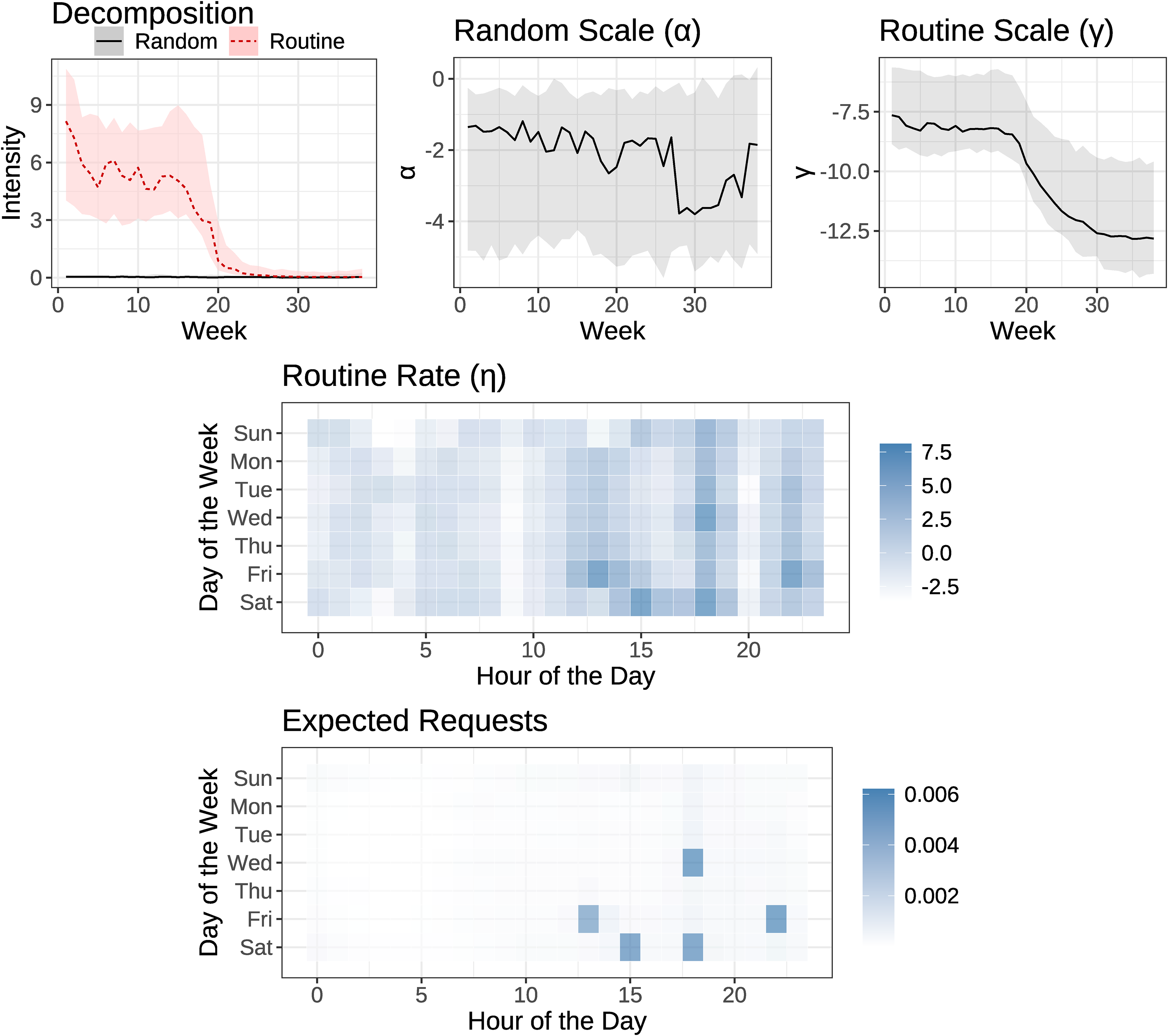
In Figure 4, we plot the key model estimates for a simulated individual for whom routine behavior emerges over time. Specifically, this individual was simulated by drawing day-hour request times in two ways: For the first half of the data (i.e., before week 19), each week, we drew five day-hours completely at random and assumed the individual makes one request at each of these five day-hours. Since the five day-hours are drawn anew each week, there is no pattern to this individual’s usage, and thus the model should capture this as random activity. Then, at week 19, we simulate this user suddenly adopting a routine. To simulate routine usage, we first drew a set of five random day-hours (e.g., Sunday at 2 p.m., Tuesday and Wednesday at 8 p.m., and Thursday at 8 a.m. and 6 p.m.) and then assumed that the user requests a ride at these same five day-hours each week. Since the user is making requests at the same times, week over week, the model should detect that a routine has emerged around week 19.

Figure 4.

Simulated Case: Random, Then Routine.

In the top-left panel of Figure 4, we plot the posterior median estimates of ${\mathrm{E}}_{\mathrm{iw}}^{\mathrm{Random}}$ (black/solid line) and ${\mathrm{E}}_{\mathrm{iw}}^{\mathrm{Routine}}$ (red/dashed line). To the right of the decomposition, we show the posterior median estimates of the random scale parameter, α_i(w), and the routine scale parameter, γ_i(w). Finally, below those, we show the posterior median estimate of the routine rate η_i(j), plotted as an intensity over day-hours, and below that, the model's expectations for when this user will request rides during the last week of the training data (w = 38).

Figure 4 shows that the model is correctly able to parse this user's behavior. In the decomposition panel, the random component ${\mathrm{E}}_{\mathrm{iw}}^{\mathrm{Random}}$ is high at the start, capturing around five rides per week. We can also see this reflected in the relatively high value of the random scale, α_i(w). Then, in the middle, we see a sudden shift, with ${\mathrm{E}}_{\mathrm{iw}}^{\mathrm{Random}}$ falling to zero and ${\mathrm{E}}_{\mathrm{iw}}^{\mathrm{Routine}}$ rising to around five, corroborating the model's ability to detect routines. These changes are driven by changes in the scale parameters, α_i(w) and γ_i(w): since the request times became consistent week over week, γ(w) increases, meaning the day-hour rate of the model is dominated by η_i(j), rather than μ(j). The relative smoothness of these trajectories, especially γ_i(w), is driven by the GP assumption for these terms, which smooths over time, with a degree of smoothing governed by the GP's length-scale parameters, ρ_α and ρ_γ. Finally, the times that the user is expected to request a ride are captured in the user's routine rate, η_i(j), for which there are five peaks in usage. These peaks, when combined with the routine scale γ_i(w) in week 38, translate exactly to five expected requests at exactly the hours simulated: Sunday at 2 p.m., Tuesday and Wednesday at 8 p.m., and Thursday at 8 a.m. and 6 p.m.

Case 2: Routine, then Churn

Figure 5 presents the results for a different simulated user, who first exhibited routine behavior (generated analogously to the last 19 weeks of the simulated customer in case study 1) but then stopped using the service altogether. Although our model is not explicitly designed to detect churn, inactivity can be captured in our framework when both scaling terms become very negative, implying zero expected requests. Indeed, this is exactly how the model behaves. The first panel shows that the decomposition correctly captures, at first, a high level of routine usage, which then dips to zero at the midpoint, when the user churns. Looking at the model components, we see that this pattern of routine requests is driven by the routine scale parameter, γ, which starts out relatively high (when the user is active), but then plummets and stays low until the end of the data. Again, the routine rate, η, can recover the correct routine for this user, with five peaks (Friday at 1 p.m., Saturday at 3 p.m., etc.). However, as reflected in the bottom panel, when that routine rate is combined with a very negative routine scale, we see that the model predicts essentially no requests for the last week of the data, when the customer becomes inactive. ²⁰

Figure 5.

Simulated Case: Routine, Then Churn.

Results

Having established the model's ability to separate routine behavior from random behavior, and its ability to accurately recover routines across different data settings, we next describe the results from the real data, estimated on the full sample of 2,000 customers over the period of 38 weeks used for model calibration.

Model Estimates

We first describe some of the population-level parameter estimates which characterize usage patterns broadly; for example, what days and times exhibit the highest level of usage across customers, and how often users exhibit random versus routine behavior. We then describe some individual case studies, exploring the degree of routineness and the specific routine patterns for individual consumers.

Population patterns

There are two main population-level parameters of interest: the population-level rate parameter, μ(j), which governs when users tend to take rides (randomly), and the correlation matrix Ω from the day-hour kernel, which describes how different days are related to one another. We plot the posterior means of these quantities in Figure 6.

Figure 6.

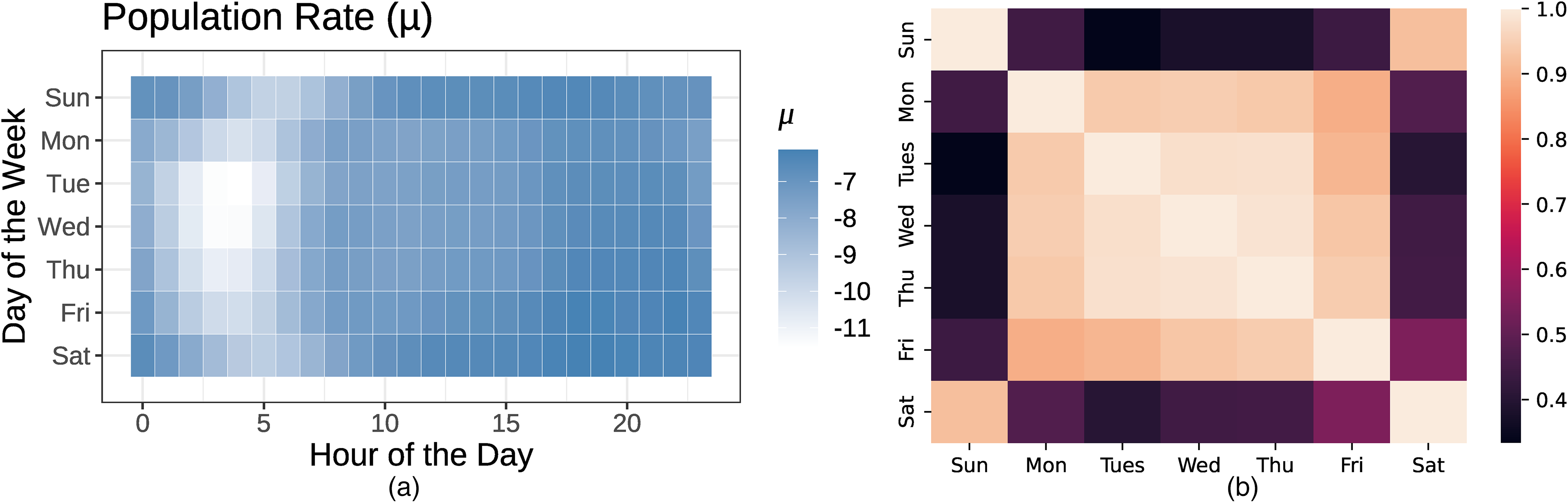
Posterior Means of μ(j) and Ω.

Some intuitive patterns emerge. First, from the posterior mean of μ(j) (Panel A), we see that random needs tend to arise during all times, except in the middle of the night (i.e., hours 2–5, or 2 a.m. to 5 a.m.). This pattern is moderated somewhat on the weekends, when travel times shift a bit later, and when there is a noticeable drop in usage at 4 a.m., corresponding to the closing time of many bars in New York City. On weekdays, we also observe a slight increase in usage of the service in the evenings, but the daytime variation is much less stark than the variation between day and night. Similarly, the correlation matrix (Panel B) captures the expected pattern that weekdays tend to be more similar to one another than to weekends. Saturday and Sunday are correlated, as are Friday and Saturday.

Another key output of our model is the decomposition of usage into routine and random requests. Figure 7 shows the joint distribution of the two parts ${\mathrm{E}}_{\mathrm{iw}}^{\mathrm{Routine}}$ and ${\mathrm{E}}_{\mathrm{iw}}^{\mathrm{Random}}$ in the last week of our data. We find an L-shaped distribution, suggesting that heavy-usage customers are either primarily routine or primarily random but rarely both. Most customers fall in the lower-left part of the figure, with few requests per week, balanced between random and routine. Although Figure 7 shows the decomposition pattern for the last week of the data, we also find similar weekly decompositions throughout the data period.

Figure 7.

Joint Distribution, ${\mathrm{E}}_{\mathrm{iW}}^{\mathrm{Routine}}$ and ${\mathrm{E}}_{\mathrm{iW}}^{\mathrm{Random}}$ .

Finally, the combination of routine and random usage, ${\mathrm{E}}_{\mathrm{iw}}^{\mathrm{Routine}}+{\mathrm{E}}_{\mathrm{iw}}^{\mathrm{Random}}$ , should capture overall usage (i.e., E[y_iw]). Indeed, we find that to be true: in-sample, the correlation coefficient between expected usage and actual usage is r = .947, p < .001, reflecting very good fit.

Individual customers’ routines

We zero in on the individual-level parameters to illustrate the insights provided by the model. Relative to the simulated examples, the results on real users are less clean-cut in their interpretation, but they still offer valuable customer-level insights. In Figures 8 and 9, we show the same posterior estimates and decompositions for two real customers, as we did for the simulated case studies in Figures 4 and 5.

Figure 8.

Real User: Commuting Routine.

Figure 9.

Real User: Random Usage.

Figure 8 provides an example of a very common type of routine: commuting. As shown in the decomposition, this customer is a fairly heavy user, making roughly 14 ride requests per week, with a high level of routine usage. This routine usage tends to cluster around commuting hours, 8 a.m. and 5 p.m., as can be seen both in the routine rate and in the expected numbers of requests. In contrast, Figure 9 presents a customer with a random pattern of usage. This customer transacts less frequently than the first customer. In the decomposition, we see the random component trending upward toward the end of the calibration window, driven by the increase in this customer's random scale. That the model captures this increase in usage with the random scale suggests that the day-hour pattern of those interactions is not consistent, week over week. While the model does still estimate a routine rate, η_i(j), when combined with the customer's very low routine scale γ_i(w), we see that the customer's expected day-hour pattern of usage is very diffuse, very much resembling the population pattern shown in Figure 6.

Heterogeneity in Routines: Uncovering Routine Types

While the case study in Figure 8 captures an intuitive and common routine, other users might have different routines. To understand the typical types of routines present in our data, we clustered our posterior median estimates of customers’ routines, η_i(j). Specifically, we focused on those customers who had at least five routine rides in total over the calibration period (i.e., $\sum _{\mathrm{w}=1}^{38}{\mathrm{E}}_{\mathrm{iw}}^{\mathrm{Routine}}\ge 5$ ). This filtering ensures that the η_i(j) parameter captures a meaningful routine, ²¹ and it resulted in 1,042 customers. Then, we performed k-means clustering on the estimated η_i(j) parameters and uncovered seven distinct routine types in ridesharing behavior, which we labeled according to the routine pattern and summarize in Figure 10. ²²

Figure 10.

Heterogeneity in Routines: Routine Cluster Centroids.

We see that although commuting is a common routine type, there are also other common routines. We find two types of likely leisure-oriented routines: The “Nights and Weekends” (14% of customers) customers primarily make requests at night, and especially on the weekends. The “Work Hard, Play Hard” (17% of customers) cluster exhibits weekend usage that peaks between midnight and 4 a.m. (the closing time of most bars in New York City) and weekday morning and nighttime usage. There are also two clusters that use the service only during one part of the day, either just in the morning (“At Dawn”; 10%) or just in the evening (“Evenings”; 9%). Understanding this diversity of routines is a key benefit of our individual-level model. For example, in this case, realizing the magnitude of the number of “half commuters,” like the “At Dawn” and “Evenings” clusters, spurred our partner company to try to understand how it can capture the full commute for these groups of customers. We return to these routine types, and explore their differential value to the company, subsequently.

Model Validation

Before exploring the implications of routineness for CRM, we first validate the model by examining its ability to predict our holdout data. Mechanically, making predictions from the model is straightforward. Since μ(j) and η_i(j) do not vary over weeks, the only two components of the model that need to be projected forward are α_i(w) and γ_i(w). To do so, we utilize the fact that GPs are marginally Gaussian to derive the posterior predictive values, given what we previously observed. Here, we focus on doing this for γ_i(w), but the math is analogous for α_i(w). Let $\mathrm{w}*$ indicate a new week that we want to make a prediction for, having observed weeks w = (w₁, …, w_W), with estimated function values γ_i(w). Then ${\gamma }_{\mathrm{i}}(\mathrm{w}*)\sim \mathrm{N}(\mathrm{m}*,\mathrm{s}*)$ , where

$$\mathrm{m}*={\gamma }_{0\mathrm{i}}+\mathrm{K}(\mathrm{w}*,\mathbf{w})\mathrm{K}(\mathbf{w},\mathbf{w}{)}^{-1}[{\gamma }_{\mathrm{i}}(\mathrm{w})-{\gamma }_{0\mathrm{i}}],$$

(16)

$$\mathrm{s}*=\mathrm{k}(\mathrm{w}*,\mathrm{w}*)-\mathrm{K}(\mathrm{w}*,\mathbf{w})\mathrm{K}(\mathbf{w},\mathbf{w}{)}^{-1}\mathrm{K}(\mathbf{w},\mathrm{w}*),$$

(17)

and where K(w, w) is the kernel matrix (on the training data), $\mathrm{K}(\mathrm{w}*,\mathbf{w})$ is the vector formed by evaluating the kernel $\mathrm{k}(\mathrm{w}*,\mathrm{w})$ for all $\mathrm{w}\in \mathbf{w}$ , and likewise for $\mathrm{K}(\mathbf{w},\mathrm{w}*)$ . Examining this equation closely reveals an important feature of GP models with stationary kernels, like our exponential kernel: when forecasting far away from observed data, GPs revert to the mean. This reversion is driven by $\mathrm{K}(\mathrm{w}*,\mathbf{w})$ going to zero when the inputs are far apart.

Using this forecasting machinery, we focus on two types of predictions: First, we predict how many sessions someone will have in the future. Second, and more pertinent to our research objective, we predict when someone will request rides, in terms of day-hours of a particular future week. We compare the predictive performance of the model to four benchmarks:

Nonroutine Usage (NR): A version of our model with the routine term set to zero, equivalent to a Poisson model with rate ${\lambda }_{\mathrm{it}}^{\mathrm{NR}}=\exp [{\alpha }_{\mathrm{i}}(\mathrm{w})+\mu (\mathrm{j})]$ . Comparing the performance of the full model with this benchmark gives a sense of what the routine part of the model captures. ²³

No Day-Hour Variation (NDH): A version of our model with all j terms eliminated, equivalent to a Poisson model with rate ${\lambda }_{\mathrm{it}}^{\mathrm{NDH}}=\exp [{\alpha }_{\mathrm{i}}(\mathrm{w})]$ . Comparing the full model with this model gives a sense of what adding day-hour variation captures.

Pareto/GGG: The Pareto/GGG model of Platzer and Reutterer (2016), as implemented in the BTYDPlus package.

Long Short-Term Memory (LSTM): An LSTM deep learning model, similar to Sarkar and De Bruyn’s (2021) LSTM for direct marketing, but with the objective of predicting which times in a week a user will request a ride. For each individual in the data, we train an LSTM with the full 38-week calibration data, then use a sliding window of data to predict, in the subsequent weeks, which day-hours are most likely to have a ride request. ²⁴

Predicting volume of requests

First, we consider the task of predicting how many sessions each customer will have during the ten-week holdout period, ignoring the actual timing of those sessions. A priori, the accuracy of these forecasts for our models will depend on how representative past usage rates are of future usage rates, given the mean reversion property of GPs described previously. We also expect the Pareto/GGG, and buy-till-you-die models more generally, to do quite well at this task, as predicting a cumulative number of transactions during a holdout window is often the main use case for these models. For our LSTM, the loss and training procedures were focused on classifying and ranking request timing (i.e., our next prediction task), not on predicting request volume. It is not a priori obvious how well the LSTM will perform on the distinct (but related) task of forecasting request volume.

In Table 2, we show the mean absolute errors in forecasting the number of requests, where the mean is computed across customers, with their corresponding 95% confidence intervals. We can see that the forecasting results match our intuition: the Pareto/GGG and our proposed model achieve statistically indistinguishable performance. ²⁵ The other versions of our model also perform well, which makes sense, as we have removed sources of day-hour variation but left the week-over-week variation components intact. The fact that these versions perform marginally worse is suggestive of the additional predictive benefit of including day-hour information. Finally, the LSTM performs quite badly. As we describe in more detail in the Web Appendix, this poor performance is likely the result of two aspects of how the LSTM was trained: First, its loss is focused on the probability that a request occurs in a given day-hour. Second, the LSTM uses a sliding window to make “one week ahead” forecasts, which, in the holdout period, requires assuming predictions are true to forecast more than one week ahead. To get good performance on the (subsequent) day-hour prediction task, we found it necessary to set the threshold for predicting that a request would materialize to be relatively small, which, in this case, leads to overforecasting the actual volume of requests.

Table 2.

Mean Absolute Error: Predicting Number of Requests.

Proposed Model	NR	NDH	P/GGG	LSTM
7.73	8.30	8.31	7.51	26.13
[7.17, 8.28]	[7.64, 8.96]	[7.65, 8.97]	[6.97, 8.05]	[19.45, 32.80]

Notes: NR = nonroutine usage; NDH = no day-hour variation; P/GGG = Pareto/GGG; LSTM = long short-term memory. The table presents mean absolute error across customers for the number of sessions during our ten-week holdout period. Intervals are 95% confidence intervals.

Predicting request timing

Beyond just predicting how many requests a user will make each week, our model also captures when a request will occur within that week, by estimating day-hour rate terms μ(j) and η_i(j). When considering an appropriate metric for validating our model, it is important to consider the continuous nature of time. Imagine a case where a customer takes a ride at 9 a.m., but the model thought the most likely time for such a ride was in the 8 a.m. hour. In well-calibrated models that consider the continuity of time, the expected rate of transacting at 8 a.m. and 9 a.m. should be similar, given that 8:59 a.m. and 9:00 a.m. are a mere minute apart. Yet, standard classification metrics like hit rates fail to take such continuity into account. Thus, a better way to measure the quality of timing predictions is through metrics for rankings, wherein the model produces a ranking of the most likely request times, and success is measured by how highly ranked the actual request times are. In our running example, the well-calibrated model should give similar rankings to the 8 a.m. and 9 a.m. times and, thus, would score similarly well in terms of predictive ability even if the customer happened to use the service at 9:00 a.m., rather than 8:59 a.m.

We use two ranking metrics to measure how well the model predicts request times: mean average precision (MAP), and conditional precision (CP). For both metrics, higher values represent better rankings. These metrics are both standard in the literature on recommendation systems, where they are used to evaluate the relevance of a ranked list of recommended items. ²⁶ To calculate these statistics for both our model and the nested NR version, we look at the ranking implied within each week by the estimated transaction rate (i.e., λ_it and ${\lambda }_{\mathrm{it}}^{\mathrm{NR}}$ ). Because the NDH model implies a uniform rate across all day-hours, the ranking statistics are undefined for this model, and we do not include its results in this section. For the Pareto/GGG, we compute the rankings implicitly, using predictions. For each customer, we use the BTYDPlus package to draw from the posterior predictive distribution of transacts for each customer. This distribution is cumulative, reflecting the total number transactions we expect to see by time t. Thus, to get an estimated transaction rate for each hour, we evaluate the cumulative predicted transactions for each hour of the holdout period and compute cumulative differences. We then rank these hours in each week. Finally, for the LSTM, similarly to our proposed model, we form a ranking by ranking the model's day-hour estimated probabilities within each week. The results for the ten-week holdout period are shown in Table 3.

Table 3.

Holdout Ride Timing Metrics.

	Proposed Model	NR	P/GGG	LSTM
MAP	.131	.069	.043	.110
	[.124, .139]	[.064, .074]	[.041, .045]	[.076, .102]
CP	.072	.029	.016	.089
	[.066, .079]	[.025, .033]	[.013, .018]	[.076, .102]

Notes: NR = nonroutine usage; P/GGG = Pareto/GGG; LSTM = long short-term memory. The table presents MAP and CP statistics for predicting ride timing in the holdout period. Intervals are 95% confidence intervals.

First, our full model dramatically improves ride time predictions compared with the model with no individual-level routines (NR). This is not surprising: the only part of the NR model that predicts ride times is μ(j). In that sense, the NR model is assuming the same day-hour ranking across all customers, or just one “population routine,” corresponding to the day-hours that customers, in general, are likely to call rides. By comparing the full model with this baseline, we corroborate that there is rich variation in the data in terms of when individual customers request rides, highlighting the predictive validity of the routine component of the model. Our model also improves considerably on the Pareto/GGG, a model that captures regularities in transaction timing but is not specifically designed to predict day-hour patterns. Although, in the extreme, such regularities could theoretically predict transaction timing down to the day-hour, capturing regularity in ride times in our application is not sufficient to predict ride timing accurately. Finally, the LSTM, which was trained specifically for this task, performs on par with our model.

It is noteworthy that the statistics in Table 3 are modest in magnitude. For instance, the CP metric suggests that we are only able to accurately predict roughly 10% of the out-of-sample session times. An important caveat here is that these metrics ignore that some trips are routine, whereas others are not. By definition, we only expect to be able to predict the routine trip times. In Figure 11, we show evidence of this phenomenon: the more routine a person is, the higher their MAP. The plot for CP is nearly identical. These results suggest that our model does, indeed, capture session timing within weeks, when that timing is predictable.

Figure 11.

MAP by Number of Routine Rides.

Routineness and Customer Management

Having established the validity of the framework, we return to one of the central questions of the article: Can routineness help firms better understand and manage their customers? One crucial advantage of being able to distill transaction timing to a single metric—routineness—is that we can subsequently explore how routineness relates to many outcomes of interest, without needing to build new models. In this section, we start by showing that routineness is a key predictor of customer value, over and above other transaction characteristics. We then explore how routineness moderates consumers’ reactions to different aspects of the ridesharing service and how customer value varies by routine type.

Routineness and Customer Value

Overall, routine customers comprise a significant part of the value in our sample: the 20% of customers who, during the calibration period, had on average one routine request per week (or at least 38 routine requests) make 53% of all sessions and 51% of the total revenue in the holdout period. Alone, these statistics are suggestive, but limited: is it these customers’ routineness that explains their high out-of-sample value, or merely their high overall request rates? To understand whether routineness explains value over and above other summaries of transaction behavior, we turn to regression analysis. Specifically, we consider the routineness of each user at the end of the calibration period (i.e., ${\mathrm{E}}_{\mathrm{i}38}^{\mathrm{Routine}}$ , as estimated by the model) and relate it to (1) # Requests, defined as the number of requests a customer makes in the holdout period, and (2) Active, defined as whether a customer is active at all in the holdout period (i.e., a measure of ten-week retention). When modeling requests as the dependent variable, we use simple ordinary least squares (OLS); for modeling activity, we use logistic regression. In each of these regressions, we control for observable characteristics that strongly predict future value, including the number of requests the customer made in the last week of the calibration data, and the commonly used recency and frequency variables that capture how recently a customer last made a request and how many requests the customer has made previously. Moreover, to see if routineness explains behavior over and above extant summaries of transaction timing, we also include the calibration period clumpiness (H_p) and regularity (as estimated by the Pareto/GGG's k_i parameter) as predictors. ²⁷

Before describing the results, we note two important aspects of these regressions: First, routine requests are part of the total number of requests. As high usage can result from either random needs or routines, this specification allows us to understand whether having a higher routine component is incrementally valuable, over and above controlling for just the level of usage. In other words, by controlling for the number of requests in w = 38, we are trying to determine whether the “shape” of within-week usage, in terms of request timing, matters for explaining future customer value. Second, the inclusion of recency and frequency metrics is especially important here: a litany of models in customer base analysis have shown that these metrics are key summary statistics for predicting repeat purchasing (e.g., Blattberg, Neslin, and Kim 2008; Fader, Hardie, and Lee 2005; Schmittlein, Morrison, and Colombo 1987). If mere habit (in the “buying habit” sense of the word) were the primary driving force behind customer value, we would expect these two statistics to explain much of the variation in future transactions. Thus, by incorporating these measures in the model, we can establish whether routineness matters, beyond what mere habit would already predict.

Table 4 presents the results of these regressions. We estimate each model three times: omitting the routineness metric (Columns 1 and 4), measuring the dependent variable using the entire holdout sample of ten weeks (Columns 1–2 and 4–5), and measuring the dependent value using the last month of the holdout data (i.e., the last five weeks, Columns 3 and 6). The intent behind splitting the dependent variable in this way is to assess how robust routineness is in explaining short- and mid-term customer behavior. We find that higher routineness is positively and significantly associated both with the number of requests a customer makes and with the customer being active at all. Furthermore, compared with the simpler models (Columns 1 and 4), routineness not only improves model fit but also is the only metric among all transaction timing metrics considered that positively and significantly explains customer activity levels, even in the mid-term. In summary, even after controlling for the number of requests a customer made at the end of the training data, standard recency and frequency measures from the CRM literature, and clumpiness and regularity, we find that number of routine requests is positively, significantly, and incrementally associated with higher request rates and a higher tendency to remain active, suggesting that customers with routines are more valuable.

Table 4.

Relationship Between Customer Value and Routineness.

	Dependent Variable:
	No. of Requests OLS			Activity Logistic
	(1)	(2)	(3)	(4)	(5)	(6)
Weeks of Test Data	All 10	All 10	Last 5	All 10	All 10	Last 5
Requests (w = 38)	3.838***	1.614***	.375**	.611***	.461***	.203***
	(.184)	(.241)	(.154)	(.103)	(.106)	(.056)
Recency	−.238***	−.284***	−.157***	−.140***	−.134***	−.123***
	(.045)	(.043)	(.028)	(.010)	(.010)	(.010)
Frequency	.130***	.097***	.052***	.0003	−.002	.002
	(.008)	(.008)	(.005)	(.002)	(.002)	(.002)
Regularity (k)	10.533***	4.511**	2.401*	.313	.005	.407
	(1.986)	(1.952)	(1.244)	(.463)	(.484)	(.395)
Clumpiness (H)	9.269***	8.443***	4.845***	−1.491***	−1.520***	−.628*
	(1.918)	(1.836)	(1.170)	(.380)	(.381)	(.326)
Routine (w = 38)		5.216***	2.685***		1.035***	.262**
		(.385)	(.245)		(.328)	(.124)
Observations	2,000	2,000	2,000	2,000	2,000	2,000
R2	.540	.579	.429

*p < .1. **p < .05. ***p < .01.

Notes: Intercept omitted for clarity. The table presents regressions of future activity—either number of future sessions (Models 1–3) or a binary measure indicating any activity at all (Models 4–6)—on customer-level summary statistics, including regularity, clumpiness, and routineness. The dependent variable is measured either over our entire holdout period (ten weeks), or just in the last five weeks of the holdout period. Standard errors are in parentheses.

Routines and Other Customer Behaviors

Next, we consider whether understanding customers’ routines can be useful for customer management in ways beyond predicting activity levels. In particular, we consider two related questions: First, do highly routine customers interact with the firm's service differently than nonroutine customers? And second, do customers behave differently during their routines? We hypothesize that customers whose usage stems primarily from a routine may not only be more likely to engage in activities that are directly valuable to the firm but also react differently to various aspects of the firm's service, like pricing and service failures (e.g., pickup and drop-off delays). There may also be differences between routine and nonroutine users in terms of which aspects of the service are more important to them. For instance, users who routinely rely on the service may place higher importance on things like convenience of trips. Such effects may exist not just across customers but also within customers. For example, if a price change or service failure is associated with a trip that is part of a customer's routine, the customer may react differently than if the price change or service failure were associated with a nonroutine trip. The direction of these within-customer effects is not a priori obvious: while the automaticity of routines implies that usage is stickier regardless of variability in service, suggesting that customers may be less sensitive to service quality during their routines, it is equally plausible that the high degree of familiarity customers have with service during their routines may exacerbate their reactions to any deviations from normal service.

To explore these hypotheses, we need to be able to quantify the overall routineness of a given customer and the degree to which a given trip is part of that customer's routine. Both quantities are easily derived from our model. The former is what we previously referred to as (weekly) routineness, measured by ${\mathrm{E}}_{\mathrm{iw}}^{\mathrm{Routine}}$ . The latter we will refer to as “trip routineness”: given an observed trip occurs during week w, day-hour j, the trip routineness is the expected number of routine requests estimated by the model at that time, ${\mathrm{E}}_{\mathrm{iwj}}^{\mathrm{Routine}}=\exp [{\gamma }_{\mathrm{i}}(\mathrm{w})+{\eta }_{\mathrm{i}}(\mathrm{j})]$ .

To understand how these two aspects of routines connect to the company's service, recall that our data include information about the rides that users requested. Some of these variables are characteristics of the proposal, including the cost to the user (Price), the time until the driver can pick the customer up (Driver ETA), how long the customer will have to walk to get the ride (Pickup Walking Dist.), the expected time and total distance of the trip (from which we compute Speed), and the number of passengers for that request (# Passengers). We observe these characteristics for all the requests in the data. Moreover, for rides that were realized (i.e., requests that ended up in a trip), we observe variables that capture the quality of the ride. These include whether the driver picked up the rider on time (Pickup Delay, which we measure in minutes), whether there were delays in the trip (Dropoff Delay), how far the rider had to walk from their drop-off to their final destination (Dropoff Walking Dist.), and whether there were other passengers in the car during the trip (# On-board [Pickup], # On-board [Dropoff], and Max On-board). ²⁸ Based on these data, we ask two questions: (1) How likely is a customer to accept a proposal, and, particularly, a less favorable proposal? and (2) Given that a customer accepts a proposal (i.e., takes a ride), how likely is that customer to request a ride again within seven days, particularly after a service failure? More importantly, we explore how the two types of routineness explain and moderate these dependent variables.

To answer these questions, we run four separate OLS regressions, the results of which are shown in Table 5. ²⁹ The dependent variable in each regression is either accepting a proposal or requesting again within a week. In the first two regressions (Models 1 and 2), the key independent variable of interest is the routineness of each customer at the end of our calibration window, and the unit of analysis is rides requested or taken during our holdout window. This setup allows us to address the “between-customers” question: Does a customer's current period routineness explain their subsequent behavior? In these regressions, we include customer-level random effects to control for other unobserved differences across customers. In the second two regressions (Models 3 and 4), the key independent variable of interest is trip routineness, and the analysis is done at the level of requests within our calibration period. We focus here on in-sample rides to ensure that our routineness metric is accurately characterizing the nature of each request. This setup allows us to address the “within-customers” question: Do customers behave differently when a trip is part of their routine? Since trip routineness is measured at the request level, we use customer-level fixed effects to control for potential customer-specific unobservables. In all four regressions, we also include variables describing the proposal. In the “request again” analyses, which condition on a customer actually having completed the trip, we include variables describing the completed trip. Finally, to understand the potential moderating role of routines in explaining these outcomes, we include interactions of all of proposal and trip-related variables with the focal measure of routineness.

Table 5.

Modeling Accepting a Proposal and Requesting Again Within Seven Days as a Function of Routineness.

	Customer Routineness (Between-Customers)		Trip Routineness (Within-Customers)
	Accept Proposal	Request Again	Accept Proposal	Request Again
	(1)	(2)	(3)	(4)
A: Proposal Characteristics
# Requests (Week 38)	−.019	.089***
Routineness	.077***	.052***	.051***	.020***
Price	−.031***	−.014***	−.071***	−.022***
Driver ETA	−.050***	−.0004	−.089***	.001
Speed	.083***	−.010	.048***	−.006
Pickup Walking Dist.	−.041***	−.002	−.021***	.001
# Passengers	−.003	.006	.009***	.012***
Routineness × Price	−.005	.014***	.018***	.016***
Routineness × Driver ETA	.011***	.001	.003	−.0001
Routineness × Speed	.142***	−.021	.086***	−.013
Routineness × Pickup Walking Dist.	−.009***	.0003	.002	−.001
Routineness × # Passengers	−.0004	.003	−.003	.004*
B: Realized Ride Characteristics
Pickup Delay		−.007***		−.0002
Dropoff Delay		−.002		−.002*
Dropoff Walking Dist.		−.003		−.002*
# On-board (Pickup)		−.004		−.003*
# On-board (Dropoff)		.001		.001
Max On-board		.003		−.002
Routineness × Pickup Delay		.005**		.001
Routineness × Dropoff Delay		.001		.001
Routineness × Dropoff Walking Dist.		.001		.001
Routineness × # On-board (Pickup)		.003		.002
Routineness × # On-board (Dropoff)		−.0002		.00003
Routineness × Max On-board		−.002		−.001
Customer Effects	Random	Random	Fixed	Fixed
Other Controls	Yes	Yes	Yes	Yes
Observations	38,166	14,704	113,042	73,630
R2	.051	.093	.070	.015

*p < .1. **p < .05. ***p < .01.

Notes: Customer routineness is measured as predicted routineness at the end of the calibration period (week 38). All models include a user-level random effect and control for the properties of the focal ride. Models 1 and 2 analyze data from the holdout period (weeks 39–48); Models 3 and 4 analyze data from the calibration period (weeks 1–38). The full set of control variables can be found in Web Appendix I. The variables in Panel A are characteristics of a proposal; Panel B shows variables associated with only realized trips. R² values are projected R², meaning the variance explained beyond the customer effects. The predictors in both models were standardized to improve readability.

Focusing first on the between-customers results, we see that highly routine customers, as measured by week 38 routineness, are indeed different in their holdout behavior. Such customers are more likely to accept proposals in general (OLS coefficient β = .077, p < .01), and more likely to make requests within a week of any given completed trip (β = .052, p < .01). In terms of accepting proposals, while longer driver estimated time of arrival (ETA) is associated with lower acceptance rates (β = −.050, p < .01), there is a positive interaction with routineness (β = .011, p < .01), suggesting routine customers are more willing to wait for their rides to come. However, more routine customers appear to especially prefer faster speeds (interaction β = .142, p < .01) and shorter walking distances (interaction β = −.009, p < .01). This pattern of moderation is consistent with routine customers caring more about convenience-related variables. In part, this could be driven by self-selection: customers do not adopt a routine if rides are inconvenient for them. In terms of requesting again within a week, we see a prominent effect of week 38 routineness on two very important service variables: price and pickup delay. While higher prices and longer delays are both associated with lower likelihood of returning to the service (β = −.014 and −.007 respectively, both with p < .01), routineness again moderates these negative effects (interactions β = .014, p < .01 and β = .005, p < .05, respectively), suggesting that the stickiness of routines makes these customers more resilient to these negative aspects of service. Taken together, these between-customers results suggest that cultivating routine customers may be valuable for the firm in myriad ways.

Turning to trip routineness (i.e., the within-customers results), we again find positive and significant effects of routineness (β = .051 for accepting proposals, and β = .020 for requesting again, both with p < .01). These main effects suggest that, for trips that are part of a customer's routine, the customer is more likely to accept the proposal, and more likely to request again within a week of the completed trip. We also see that the routineness of a trip appears to moderate the negative effect of price: while customers in general are less likely to accept higher-priced proposals (β = −.071, p < .01) and to ride again (β = −.022, p < .01) after taking a higher-priced ride, these effects appear to be dampened when that ride is part of the customer’s routine (interactions β = .018 and .016 respectively, both p < .01). There is also a positive interaction between the routineness of a trip and the speed of the proposal: when a customer requests a routine trip, they are more likely to accept the proposal if the speed is high (interaction β = .086, p < .01). Intuitively, customers are familiar with trips in their routine and, thus, more sensitive to the details of those trips. This pattern of effects suggests ways that the firm can explore optimizing service around customers’ routines, by, for example, offering faster service at premium prices for customers during their most routine times.

Segmentation by Routine Types

Recall that a key benefit of our framework is that it not only yields an overall metric of routineness (of a ride, or a customer, as we leveraged in the previous analyses) but also enables us to uncover common routines in the data. In our application, we found that there are seven common routine types, which we summarized in our section on model results. Given these different routine types, we next consider whether customers with different routines differ in other significant ways. We find that these routine types differ not only in when they typically take rides but also in many other behaviors and typical ride characteristics. For instance, the more casual routine types (i.e., “Work Hard, Play Hard” and “Nights and Weekends”) tend to take longer and more expensive trips (higher ETA). Commuters, in contrast, tend to take cheaper, solo trips. ³⁰ More interestingly, though, we also find that users with different routines systematically differ in their value to the company. In Figure 12, for each routine type, we show means and standard errors of that type's (1) proposal acceptance rate; (2) future value, as measured by the total amount spent during our holdout period; (3) proportion of (holdout) rides that came from nonroutine usage, as estimated by our model; and (4) number of requests made during the holdout period. We find striking differences across the routines. For example, the casual clusters had a much lower probability of accepting rides and generated significantly lower value during our holdout period. In contrast, the “Evenings” routine appears to be the most valuable: these customers had a higher probability of accepting rides, took more rides, and spent more money during that same period. Interestingly, a higher share of their overall usage was also attributed to their routine. Commuting clusters also appear more valuable, especially those that also incorporate evening usage. In summary, these results suggest not only that there is significant heterogeneity in routine types but also that these routine types are associated with substantially different behaviors, suggesting a role for routines to play in segmenting and targeting customers.

Figure 12.

User Behaviors, by Routine Type.

Additional Analyses: Who and What

Until now, our analyses have proceeded by first identifying routines in terms of when customers interact with the firm, then linking those temporal routines to relevant outcomes. This approach raises two questions: First, can we predict who tends to develop routines? And second, beyond timing, is there any value in considering routines in terms of what customers do during those interactions? In our context, ridesharing, the “what” of interest is where customers are traveling: customers may always request a ride at the same time, but they may go to the same place or different places.

To answer the “who” question, we examined whether any proposal characteristics, averaged over the calibration period, are predictive of high customer routineness at the end of the training period (week 38). We find several suggestive patterns: first, routine customers tend to have taken lower-priced rides, with fewer other passengers, and shorter walking distances. These results may be indicative of causality, whereby riders develop routines because they are given cheap, convenient trips, or selection, wherein riders with routines happen to take rides during lower-priced, high-supply times. Interestingly, these rides also tended to be longer rides, with higher driver ETAs, which is consistent with travel during peak times, and the presence of many commuters in our data. These results are described in more detail in Web Appendix K.

To answer the “what” question, we used trip location data to derive two metrics of location consistency, which capture how often each rider travels between the same locations. We then analyzed the relationship between location consistency, (temporal) routineness, and customer value. We find that location consistency is neither particularly predictive of (timing) routineness nor predictive of customer value after controlling for routineness. These results suggest that, at least in the context of ridesharing, understanding consistencies in when someone uses the service is more important than understanding consistencies in where they are going. These results are described in more detail in Web Appendix L.

Discussion

Summary and Contribution

Our work makes two primary contributions. First, from a methodological point of view, to the best of our knowledge, this is the first article to model customer-level routines. To do so, we leverage a Bayesian nonparametric GP with a unique kernel structure aimed at estimating temporal routines, nested within a Poisson process. This model can flexibly capture varying routines across customers with high accuracy. Additionally, it yields a customer-level decomposition of usage into a part that is routine and a part that is random, allowing us to quantify the degree of a customer's routineness. Substantively, we apply the model to data from Via, a ridesharing company, and show that we can capture managerially interesting routines. We find that our model-based routineness metric is strongly predictive of customer value, insofar as it is a positive and significant predictor of both future usage and retention. Moreover, this effect is robust, even over longer time horizons, and after controlling for the level of usage, other typical CRM controls, and extant transaction timing metrics. Stated differently, this result is noteworthy because it suggests that the temporal shape of usage matters: highly structured usage is more valuable than random usage. While we apply our model in the context of ridesharing, the model we propose is general and can be applied to usage or purchase data in many business settings.

Beyond our focus on the relationship between routineness and customer value, we also present results that both validate routineness as a construct and establish its more wide-ranging importance in customer management. We show that routine customers are better customers in ways that stretch beyond just lifetime value: they appear to be generally less price sensitive and more robust to some types of service disruptions. Our results suggest that firms that understand their customers’ routines can optimize the provision of services around those routines. Conceptually, we differentiate routineness from constructs like clumpiness and regularity. Finally, we show that routines represent an important source of heterogeneity that can be useful for segmentation and targeting.

Limitations and Future Research

We view our work as an initial foray into the topic of modeling and measuring customer routines and establishing their importance for customer management. As such, there are several limitations of our work, which represent promising directions for future research, to expand both our modeling capabilities and our understanding of when and why routines matter.

From a methodological perspective, scalability of our framework is a limitation. While the run time of the framework is feasible, estimating our model in a fully Bayesian fashion on a large sample of customers can be costly, as the run time is superlinear in the sample size (see the simulations in Web Appendix B). In practice, our partner company implements our model on a large sample of data. Our simulation results suggest estimating the model on a sample of consumers is a reasonable solution: the quality of insights from small batches is equivalent to larger data sizes. Thus, running the model in parallel with 10 compute nodes for 1 million customers using 20 weeks of data would take approximately 14 hours, which we argue is quite feasible for most companies with established data science tools. Alternatively, future research may examine new avenues for improving scalability, including variational Bayesian methods for inference (Hoffman et al. 2013), or stochastic gradient Hamiltonian Monte Carlo methods (Dang et al. 2019). Our methodology is also limited in that it does not incorporate an explicit latent churn process. While we have provided some evidence that the framework can detect customer inactivity, our model performs best when the purchasing process is relatively stationary.

From a substantive perspective, an area we leave unexplored is the emergence of routines: while we show suggestive results about which customers and trips are more likely to be routine, these patterns are merely suggestive. Our analysis is not causal, and thus cannot establish whether these are indeed drivers of routines. However, given our findings that routine customers are better customers, cultivating routines may be of key interest to companies, and understanding how to do so is a fruitful area for future research. Likewise, while we show suggestive evidence that routine customers are less price sensitive, price endogeneity is an important issue that we cannot fully resolve with our data. Price experiments should ideally be run to better understand how price sensitivity varies by routineness. We leave a more complete understanding of the relationship between price sensitivity and routines to future studies.

There are several other limitations of our analysis. For instance, our main model captures requests, not actual rides taken. Whether a rider takes a ride may, in part, be driven by supply-side factors like availability of a ride. In turn, whether the service was able to meet a rider's demands in the past may affect how routinely the customer requests rides in the present, leading to perfectly routine behaviors appearing less routine in our model. Another limiting factor in our analysis is our focus on temporal routines. While we provide some evidence that consistency in terms of what customers do is less important, there may still be value in jointly modeling “when” and “what.” We leave building such a joint model for future research. Relatedly, because our model focuses just on timing, we cannot differentiate between different subroutines: drawing on an example from our introduction, if a customer had a routine going to work, and another routine going to yoga class, our model results would blend these into just a single routine. Finally, our understanding of routines more generally is limited by the fact that we only observe rideshare usage by a single company: more comprehensive panels featuring more alternatives may shed additional light on customer routines and how they drive consumer choice. We hope these limitations spur additional study of customer routines.

Supplemental Material

sj-pdf-1-mrj-10.1177_00222437231189185 - Supplemental material for Detecting Routines: Applications to Ridesharing Customer Relationship Management

Supplemental material, sj-pdf-1-mrj-10.1177_00222437231189185 for Detecting Routines: Applications to Ridesharing Customer Relationship Management by Ryan Dew, Eva Ascarza, Oded Netzer and Nachum Sicherman in Journal of Marketing Research