Measuring Evidence for Mediation in the Presence of Measurement Error

Abstract

Mediation analysis empirically investigates the process underlying the effect of an experimental manipulation on a dependent variable of interest. In the simplest mediation setting, the experimental treatment can affect the dependent variable through the mediator (indirect effect) and/or directly (direct effect). However, what appears to be an indirect effect in standard mediation analysis may reflect a data-generating process without mediation, including the possibility of a reversed causal ordering of measured variables, regardless of the statistical properties of the estimate. To overcome this indeterminacy where possible, the authors develop the insight that a statistically reliable total effect, combined with strong evidence for conditional independence of the treatment and the outcome given the mediator, is unequivocal evidence for mediation as the underlying causal model into an operational procedure. This is particularly helpful when theory is insufficient to definitely causally order measured variables, or when the dependent variable is measured before what is believed to be the mediator. The procedure combines Bayes factors as principled measures of the degree of support for conditional independence, with latent variable modeling to account for measurement error and discretization in a fully Bayesian framework. The authors reanalyze a set of published mediation studies to illustrate how their approach facilitates stronger conclusions.

Mediation analysis is a tool to corroborate hypotheses about the process by which the experimental treatment brings about its effect on the dependent variable. Establishing mediation is fundamental to scientific research that seeks to understand how the world works in situations where the process connecting a manipulation to an outcome of interest is not directly observable. Understanding the process can be particularly important in marketing if an action fails to generate the desired outcome in the absence of the required mechanism. For example, Andrews et al. (2016) show that individuals in crowded areas are more likely to respond to targeted mobile ads because crowding invades their privacy and causes them to become immersed in their mobile phones (and thus be exposed to ads). Without knowing the mechanism through which crowdedness affects ad response, a marketer might decide to develop an algorithm purely based on crowdedness that targets individuals in all high-density areas, including social events or live concerts. This would be futile because individuals seek social interactions at such events (or focus their attention on the performing artist at live concerts) and thus do not experience a privacy invasion to withdraw from. Put differently, the mechanism that channels the crowdedness effect into increased ad response in some crowded areas (e.g., a train station) does not exist in other crowded areas (e.g., social events, live concerts).

Moreover, mediation is at the heart of a structural understanding of the world that would otherwise require a new theory for every manipulation studied. For example, the observations that color contrast (Thompson and Ince 2013), typicality (Landwehr, Labroo, and Herrmann 2011; Landwehr, Wentzel, and Herrmann 2013), exposure (Ferraro, Bettman, and Chartrand 2008; Landwehr, Golla, and Reber 2017), and pronounceability (Alter and Oppenheimer 2008; Song and Schwarz 2009) manipulations all bring about effects on a variety of dependent variables mediated by processing fluency parsimoniously structures our causal understanding of the world (Graf, Mayer, and Landwehr 2018). Relatedly, mediation defines subsets of variables that can be validly studied in isolation. For example, the understanding that the effect of variable production costs on demand is fully mediated by retail price allows for the exclusion of variable production costs from the price–demand model (and makes variable production costs a potential instrumental variable for price). ¹

In the context of corroborating hypotheses about unobserved processes such as mediation, it is useful to distinguish between uncertainty about the strength of unobserved connections that are beyond questioning per se and uncertainty about the connective structure itself. Empirical testing of the strength of connections in a given, undisputed model is a standard statistical exercise that may nevertheless require sophistication. Resolving uncertainty about the connective structure—and, ideally, establishing a unique causal interpretation of the connective structure supported by the data—tends to be more difficult and often beyond reach in the context of observed data. The goal of mediation analysis in practice often falls into the latter class of problems.

For example, in so-called measurement-of-mediation designs, where the mediator is measured and not experimentally manipulated, uncertainty about the connective structure (i.e., the underlying causal model) may include uncertainty about the causal ordering of measured variables, as reflected in the use of reverse mediation tests (for recent examples, see Chaxel [2016], Cunha, Forehand, and Angle [2015], Durante and Arsena [2015], Guendelman, Cheryan, and Monin [2011], and Mazar and Aggarwal [2011]).

Thus, when conducting mediation analysis, researchers may not ask for measures of coefficients in a model they know a priori. Instead, researchers may ask what model generated the data. To this end, this article provides tools and a procedure aimed at measuring data-based evidence for mediation in the context of measurement-of-mediation designs with random assignment into experimental treatments X and measurements of what may be the mediator M and the dependent variable Y.

To preview what can be expected from the application of the procedure advocated in this article, Table 1 shows that even though the studies by Shaddy and Fishbach (2017) and Yan and Muthukrishnan (2014) appear similar when the analysis is based on Baron and Kenny (1986) or Preacher and Hayes (2004), we find that the data in Shaddy and Fishbach strongly support mediation as the underlying causal data–generating mechanism, including the causal ordering of measured variables, whereas the data in Yan and Muthukrishnan (2014) do not. Consequently, the interpretation of the statistically significant indirect effect measured in Yan and Muthukrishnan as evidence of mediation must rely on prior knowledge about the data-generating causal model, and specifically about the causal ordering of measured variables and the absence of unobserved confounders between measured variables. ²

Table 1.

Examples of Results From the Extant Mediation Analysis Methods and Those From the Proposed Procedure.

	Shaddy and Fishbach (2017)	Yan and Muthukrishnan (2014)
Baron and Kenny (1986)	Indirect effect: significant Direct effect: insignificant	Indirect effect: significant Direct effect: insignificant
Preacher and Hayes (2004)	Indirect effect's bootstrapped CI excludes 0	Indirect effect's bootstrapped CI excludes 0
The proposed procedure	Substantial evidence supporting mediation	Insufficient evidence for mediation

Our contribution is the synthesis of (1) the causal identifiability of a causal chain (i.e., full mediation from observed variables; Glymour 2001; Pearl 2009); (2) Bayes factors as measures of empirical evidence supporting the restrictions implied by an unconfounded causal chain and, thus, supporting full mediation (cf. Nuijten et al. 2015); and (3) explicit models of measurement error (Bolger 1998; Cole and Maxwell 2003; Holmbeck 1997; Hoyle 1999; MacKinnon 2012) into a novel operational procedure. On the methodological side, we contribute a numerically reliable, efficient way of computing the required Bayes factor in the context of models that account for measurement error.

The user benefit from our synthesis is potentially strong empirical support for causal mediation in the form of a causal chain as the most likely among a large number of possible underlying data-generating processes. This includes an empirical confirmation of the assumed causal order of measured variables and of the absence of unobserved confounding variables. As a by-product, our procedure can establish the experimental manipulation, the mediator, and the dependent variable as different causal entities relative to the competing hypotheses that measured variables are mere manipulation checks or multiple measures of the same dependent variable.

The remainder of this article is organized as follows: First, we characterize the model discovery problem and relate our contribution to extant literature. We then develop the proposed procedure, which operationalizes a causal identifiability result leveraging Bayesian model comparison and models of measurement error. Following this, we put the procedure to practical use by reanalyzing recently published studies. Finally, we summarize in the form of a flowchart and a set of procedural steps to follow and conclude with a discussion of future research. Computer code implementing the developments in this article is available online at GitHub (https://github.com/arashl1364/BFMediate), together with a web application that provides a user-friendly interface available at Shinyapps.io (https://bfmediate.shinyapps.io/bfmediate_app). (the Web Appendix provides instructions for how to replicate selected reanalyses presented in this article based on original data sets. ³ )

Problem Characterization

Canonically, researchers seek support for the causal model depicted in the form of a directed acyclic graph (DAG) in Figure 1. In line with the vast majority of published applications, we assume linear relationships between (known functions of) measured variables (i.e., linearity in regressors). Although this is not without loss of generality, this case is practically relevant, as apparent from the mediation studies we reanalyze in the “Reanalysis of Published Studies” section. However, we subsequently accommodate nonlinear relationships between (linearly related) latent variables M and Y and their observed measures.

Figure 1.

Mediation DAG.

In this DAG, the experimentally manipulated, randomly assigned variable X exerts an effect on the dependent variable Y that consists of an indirect effect mediated by M and a direct effect β₃. Both M and Y are measured variables in the setting we study. Variables {U_M, U_Y} are unobserved causes of variation in M and Y (error terms), respectively. Variable U_X symbolically summarizes experimental manipulation and random assignment of X (as a function of U_X, X(U_X)). The DAG in Figure 1 reflects the standard assumption that U_X, U_M, and U_Y are independently distributed. ⁴ Because of random assignment, the causal effect from X to M (i.e., β₁) as well as the total causal effect from X to Y (i.e., α) can be consistently estimated. Note that for the common case of categorical X, both causal effects are nonparametrically identified without any further assumptions by random assignment of X. ⁵

If this DAG is the data-generating mechanism, it follows, first, that blocking the path through M by forcing M to take a particular value experimentally will make the effect from X to Y equal β₃ (will make the effect vanish in the case of β₃ = 0). This is the definition of mediation.

Second, if U_M and U_Y are indeed independent, it follows that both the direct effect β₃ and the indirect effect can be consistently estimated from observations of M and Y in an experiment manipulating X. Under the common assumption of a linear effect from M onto Y, the indirect effect equals the product β₁ × β₂, and the total effect α equals β₃ + β₁ × β₂ (i.e., the sum of the direct and the linear indirect effect).

However, independence between U_M and U_Y is only an assumption in standard mediation analysis, and requires that the assumed causal ordering of measured variables M and Y is correct, as well as the absence of unobserved background variables that render U_M and U_Y dependent, even conditional on the correct causal ordering. As we explain next, these possibilities call into question the interpretation of results from standard mediation analysis as data-based evidence for mediation.

Historically, mediation analysis relied on a procedure popularized by Baron and Kenny (1986). The procedure fits the regression models in Equations 1–3, where α measures the total causal effect from X to Y, and β₁ measures the causal effect from X to M, when X is experimentally manipulated and thus randomly assigned. ⁶ The coefficients β₂ and β₃ in Equation 3 have a causal interpretation only when the error terms are subject to the assumptions expressed in Figure 1 and discussed previously.

$$\mathrm{Y}={\alpha }_{0\mathrm{Y}}+\alpha \mathrm{X}+{\mathrm{e}}_{\mathrm{Y}}({\mathrm{e}}_{\mathrm{Y}}={\beta }_2{\mathrm{U}}_{\mathrm{M}}+{\mathrm{U}}_{\mathrm{Y}}),$$

(1)

$$\mathrm{M}={\beta }_{0\mathrm{M}}+{\beta }_1\mathrm{X}+{\mathrm{U}}_{\mathrm{M}},$$

(2)

$$\mathrm{Y}={\beta }_{0\mathrm{Y}}+{\beta }_2\mathrm{M}+{\beta }_3\mathrm{X}+{\mathrm{U}}_{\mathrm{Y}}.$$

(3)

Thus, the correspondence between estimates obtained from fitting Equations 1–3 to data and the structural parameters in Figure 1 is uncertain, and the scope for learning about the actual data-generating structure is limited.

Results in which the data credibly support a nonzero product β₁ × β₂ when fitting Equations 1–3 are correctly interpreted as consistent with the causal model in Figure 1; however, these results do not identify mediation as the data-generating mechanism, regardless of how much sophistication goes into assessing the statistical uncertainty in the estimate of the product β₁ × β₂ (e.g., MacKinnon, Fairchild and Fritz 2007; MacKinnon et al. 2002; MacKinnon, Lockwood and Williams 2004; Preacher and Hayes 2004; Shrout and Bolger 2002).

For example, the data-generating mechanisms depicted in Figure 2 will generally result in data that yield estimates consistent with an indirect effect when analyzed using the methods in Baron and Kenny (1986) or Preacher and Hayes (2004). These estimates, however, lack substantive meaning in both cases. In Figure 2, Panel A, what appears to be an indirect effect is spurious because there is no causal link from M to Y, and hence no causal indirect effect from X to Y via M. Thus, a potential replication study pursuing an experimental design that manipulates and randomly assigns M will not find a causal effect from M to Y. ⁷

Figure 2.

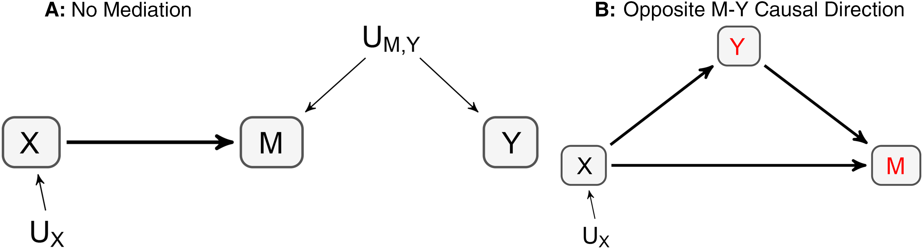
Examples of Observationally Equivalent Models to Partial Mediation.

In Figure 2, Panel B, the estimate lacks meaning because the analyst reversed the causal order of measured variables, mistaking the mediator M for the dependent variable Y, and vice versa. Again, a potential replication study pursuing an experimental design that manipulates and randomly assigns Y will not find a causal effect from Y to M. We provide numerical illustrations in the Web Appendix.

These examples highlight that estimates of a putative indirect effect should not be interpreted as evidence of mediation without at least a discussion—or, even better, an empirical assessment of the underlying causal model.

Moreover, we show in the following section that even advanced extant approaches to causal mediation analysis depend on definite prior knowledge about which measured variable is M and which is Y—knowledge that is not always available. Designs that measure the mediator only after measuring the dependent variable further complicate the definite causal ordering of measured variables based on prior knowledge (e.g., Kim, Kim, and Park 2012; Mazar and Aggarwal 2011; Shaddy and Fishbach 2017; Sussman and O’Brien 2016).

Related Literature

We organize the discussion of the literature related to our contribution using the classification scheme in Table 2. The first column in Table 2 references a selection of papers representative of the respective approaches to mediation analysis. Columns 2–5 pertain to assumptions that may be required for valid inference. The last column simply states whether a particular approach measures evidence for conditional independence between randomly assigned X and what is taken to be a measure of Y, given what is taken to be a measure of M.

Table 2.

A Comparison of the Existing Approaches in Terms of Their Assumptions for Valid Inference.

	Required Assumptions
	Asymptotic Normality	No Measurement Error	No Unobserved Confounder (UM,Y)	Causal Direction Between Measured Variables	Measures Evidence for Conditional Independence
Baron and Kenny (1986)	Yes	Yes	Yes	Yes	x
Preacher and Hayes (2004)	Relaxed	Yes	Yes	Yes	x
Muthén and Asparouhov (2015)	Relaxed	Relaxed	Yes	Yes	x
Imai, Keele, and Tingley (2010), Liu and Wang (2021)	Relaxed	Relaxed	Relaxed	Yes	x
Zhang, Wedel, and Pieters (2009)	Relaxed	Relaxed	Relaxed	Yes	x
The proposed procedure	Relaxed	Relaxed	Relaxed	Relaxed	✓

Among the approaches listed in Table 2, only the original procedure by Baron and Kenny (1986) requires asymptotic normality of the product term β₁ × β₂ for valid inference. This assumption has been relaxed subsequently using bootstrapping (e.g., MacKinnon et al. 2002; MacKinnon, Lockwood, and Williams 2004; Preacher and Hayes 2004; Shrout and Bolger 2002) or Bayesian inference (e.g., Zhang, Wedel, and Pieters 2009). However, interpreting an estimate of β₁ × β₂ as a consistent measure of a causal indirect effect requires further assumptions that pertain to structural aspects of the unobserved data-generating model: that is, a lack of measurement error in the mediator (Column 3), the absence of unobserved confounders between measured variables (Column 4), and the correct causal ordering of measured variables (Column 5). Meeting this last requirement is not trivial in behavioral studies that often only measure what may be the causal mediator M after measuring what is assumed to be the dependent variable Y (e.g., Kim, Kim, and Park 2012; Mazar and Aggarwal 2011; Shaddy and Fishbach 2017; Sussman and O’Brien 2016). ⁸

Muthén and Asparouhov (2015) relax the assumption of the absence of measurement error, advocating latent variable modeling for mediation analysis (see also Lee 2007). Imai, Keele, and Tingley (2010) and Liu and Wang (2021) alleviate the stringency of the subjective bet on the absence of measurement error and that of unobserved confounders (U_M,Y), suggesting sensitivity analyses. Finally, Zhang, Wedel, and Pieters (2009) propose latent instrumental variable modeling to overcome both assumptions.

However, as shown in Table 2, Column 5, all extant approaches rely on prior knowledge about the causal ordering of measured variables. In other words, they require a definite a priori assessment of which measured variable is the mediator M and which is the dependent variable Y. The sensitivity analysis advocated in Imai, Keele, and Tingley (2010) and Liu and Wang (2021) cannot distinguish between error correlations due to a reversed causal order or due to other reasons. The latent instrumental variable approach employed by Zhang, Wedel, and Pieters (2009) fails to identify the causal order because the instrument is latent. The Web Appendix provides numerical illustrations of how the sensitivity analysis originally proposed by Imai, Keele, and Tingley and latent instrumental variable modeling (Zhang, Wedel, and Pieters 2009) will fail to detect a misspecified causal ordering of observed variables (i.e., the case where the researcher mistakes M for Y and vice versa).

In contrast, the procedure we propose (and develop in detail in the following section) can unequivocally establish the causal chain from X through M to Y (i.e., full causal mediation) as the data-generating causal model, including the causal order of measured variables in this model (see Figure 3).

Figure 3.

DAG of Full Mediation.

The proposed procedure is best viewed as a novel operationalization of an important result in the causality and model discovery literature (e.g., Glymour 2001; Pearl 2009). In this context, we require a measure of data-based support for conditional independence between X and Y given M. Our proposed solution to this challenge relies on Bayesian model comparisons. Thus, our inferential approach is fully Bayesian.

Bayesian inference, of course, has a history in mediation analyses (e.g., Dyachenko and Allenby 2022; Muthén and Asparouhov 2012; Zhang, Wedel, and Pieters 2009). Prominently, Wedel and colleagues developed Bayesian inference for different mediation models, with single and multiple mediators, in their Bayesian analysis of variance (BANOVA) package (Dong and Wedel 2014; Wedel and Dong 2020, 2021; Wedel and Kopyakova 2022). However, to the best of our knowledge, Bayesian inference has not been applied to the problem of model identification (causal discovery) in the context of mediation analysis. While Nuijten et al. (2015) mention the use of Bayes factors to distinguish between full mediation and partial mediation, these authors do not explain that partial mediation cannot be identified from data as the underlying causal model. Moreover, Nuijten et al. develop model comparisons only for the case of directly observed variables. Another Bayesian approach that at first glance provides indirect data-based evidence for the causal chain from X through M to Y is by Dyachenko and Allenby (2022). However, we explain and numerically illustrate in the web appendix that this is not the case. In a nutshell, Dyachenko and Allenby classify observations based on relative fit compared with other observations.

Finally, while the biasing role of measurement error in the context of inference about what may be a causal indirect effect has long been recognized (Baron and Kenny 1986; Cole and Maxwell 2003), along with latent variable modeling as a viable solution (Cole and Preacher 2014; Iacobucci 2008; Iacobucci, Saldanha, and Deng 2007; Muthén and Asparouhov 2015), we need to overcome measurement error as an impediment to model discovery.

Measuring Evidence for Mediation

This section lays out the individual components of the proposed procedure to measure evidence for mediation in detail. We first summarize the basic causal identifiability argument we rely on and briefly revisit why this argument has been dismissed as impractical in the past. We then discuss the role of measurement error in the process and introduce latent variable modeling. Finally, we introduce Bayes factors as a means to operationalize the causal identifiability argument in this context, including a numerically reliable computational approach.

A basic result in the literature on model discovery establishes the unique identification of the (unconfounded) causal chain from X through M to Y (i.e., full causal mediation from data). In short, the possibility of discovering the presence of such a causal chain from data follows from the insight that if the only connection from X to Y is through M, conditioning on M will leave X and Y independent. The only other models that generate the same conditional independence relationships are a Model 1, in which Y causes M, which in turn causes X (i.e., the causal chain with reversed causal direction), and a Model 2, where M acts as a common cause to both X and Y. ⁹ However, random assignment of X rules out both of these models. In addition, a model without a causal effect from X to Y (i.e., unconditional independence between X and Y) may also yield conditional independence. However, in connection with evidence for a (total) causal effect from X to Y, conditional independence between X and Y given M uniquely establishes the causal chain (Glymour 2001, p. 33). In other words, evidence for a (total) causal effect from X to Y strengthens the previous if-statement to: If and only if the only connection from X to Y is through M, conditioning on M will leave X and Y independent. ¹⁰ Hereinafter, when we mention the unique mapping from conditional independence between X and Y given M onto the causal chain from X through M to Y, we always implicitly assume randomly assigned X and a statistically reliable total effect from X to Y.

Conditional independence between X and Y given M thus rules out all observationally equivalent models—from the perspective of inference focused on what may be an indirect effect—with the exception of the causal chain in Figure 3 (see Table 3 and the Web Appendix). Relatedly, conditional independence rules out cases where variation in M that is orthogonal to X (i.e., variation in U_M) is not causally related to Y—for example, when M is just another indicator for a latent Y, or when M is just a reflection of X (i.e., a mere manipulation check).

Table 3.

Ambiguity of the Significant Indirect Effect and Unique Model Identification from Conditional Independence.

Data-Generating Model	Significant Indirect Effect	Conditional Independence
Full mediation (Figure 3)	✓	✓
Partial mediation (Figure 1)	✓	X
M-Y unobserved confounder (Figure. 2a)	✓	X
M-Y reverse causal direction (Figure 2, Panel B)	✓	X

It is noteworthy that Baron and Kenny (1986, p. 1176) state that evidence for full mediation (i.e., evidence for a causal chain) is the “strongest demonstration of mediation” (see also MacKinnon 2012, p. 395; Shrout and Bolger 2002). Accordingly, many behavioral researchers agree that full mediation is the gold standard (e.g., MacKinnon 2012; Zhao, Lynch, and Chen 2010). However, in practice, published mediation studies often fail even to report estimates of the conditional direct effect.

Different arguments propose de-emphasizing, if not ignoring, the search for conditional independence in mediation models. The first argument relates to the drawbacks of null hypothesis significance testing (NHST). Specifically, failing to reject the absence of a direct effect using NHST (failing to reject H₀: β₃ = 0 in Figure 1) is consistent with full mediation. However, by construction, NHST does not provide a measure of data-based evidence in support of full mediation because the ex ante probability of a p-value (i.e., the probability of a p-value before the data sample is realized) is equal to its value under the null hypothesis. For this reason, Preacher and Kelley (2011, p. 97) criticize full mediation as “not expressed in a meaningfully scaled metric.”

Second, statistical tests of direct effects often suffer from low power and high sampling variability (Fritz and MacKinnon 2007; Hayes 2009; Kenny and Judd 2014; MacKinnon, Krull, and Lockwood 2000; Rucker et al. 2011; Shrout and Bolger 2002). Therefore, the absence of a direct effect as measured by these tests could be due to a lack of information in the data. Third, pointing to measurement concerns, some authors advise against testing the direct effect altogether. Specifically, Rucker et al. (2011, p. 369) argue that “the impossibility of perfect measurement, in and of itself, suggests that one cannot ever claim to have established complete mediation.”

Classical additive measurement error in the mediator M complicates standard mediation analysis following Baron and Kenny (1986) or Preacher and Hayes (2004) in two ways: First, it biases the indirect effect estimates, specifically ${\hat{\beta }}_2$ , toward zero because it inflates the mediator's variance. Second, the combination of unbiased ${\hat{\beta }}_1$ with biased ${\hat{\beta }}_2$ necessitates bias in the direct effect estimate ${\hat{\beta }}_3$ away from zero when there is no causal direct effect β₃ (Kahneman 1965). The latter confounds conditional independence and obfuscates full mediation at the causal theory level. Similar biases arise from using a categorized version of a continuous mediator, such as measures from a rating scale in the analysis (e.g., Iacobucci 2008).

We illustrate these biases with a numerical example. We simulate 500 observations from the mediation model shown in Figure 3, where conditional independence holds (X ∼ N(0, 1), β₁ = 1, β₂ = 3, β₃ = 0, Var(U_M) = 1, Var(U_Y) = 1). Next, we simulate noisy observations of M by adding measurement error ${\mathrm{U}}_{{\mathrm{m}}^{*}}\sim \mathrm{N}(0,{\sigma }_{{\mathrm{m}}^{*}}^2)$ , where ${\sigma }_{{\mathrm{m}}^{*}}^2=5$ , to M. We use the symbol ${\mathrm{m}}^{*}$ for the noisy observations. The second column in Table 4 summarizes how conditioning on ${\mathrm{m}}^{*}$ instead of M biases the estimate of the direct effect β₃ away from zero, leading to a spurious rejection of the null hypothesis β₃ = 0, and thus of full mediation. Finally, we discretize M to observations $\tilde{\mathrm{m}}$ on a seven-point rating scale based on cutoff values {−2, −.5, .5, 2, 4, 5}. Conditioning on $\tilde{\mathrm{m}}$ instead of M again results in a reliably positive estimate of β₃ (see the last column of Table 4), obfuscating full mediation as the underlying causal model. We next introduce explicit models of measurement error to avoid spurious evidence against a causal chain.

Table 4.

Direct Effect Estimates When Conditioning on the Mediator M; on M Afflicted by Measurement Error, m*; and Discretized M, $\tilde{\mathrm{m}}$ .

Conditioning Variable	M	m*	$\tilde{\mathbf{m}}$
${\hat{\beta }}_3$	−.04 (.04)	2.45*** (.08)	.67*** (.07)

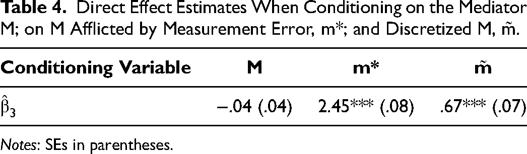
Notes: SEs in parentheses.

Measurement Error Models

We use latent variable models (LVMs) to accommodate both classical measurement error and categorized measures of continuous mediators. In contrast to previous research, LVMs here serve as a building block to model discovery. Specifically, we need LVMs to avoid spurious evidence against the causal chain from X through M to Y, as illustrated previously. Empirically, we take advantage of the fact that the majority of applications use multiple indicators for measured variables. ¹¹ In turn, when planning a study, our results support and encourage the use of multiple indicators for measured variables.

Classical measurement error

We require at least two indicators (i.e., two observed measures) for M to empirically identify measurement error independently from a potential direct effect from X to Y (β₃). With one indicator, the model is only set-identified (see the Web Appendix for a detailed characterization). The intuition is that the (measurement) error variances of multiple M-indicators and the residual variance in latent M, after conditioning on X, are jointly identified, whereas a single M-indicator cannot distinguish between residual variance in M and measurement error variance in the indicator. ¹² Regarding Y, multiple indicators are optional for (point) identification. However, when the mediator is indirectly observed through imperfect measures and there only is one indicator for Y, the conceptual distinction between M and Y no longer directly follows from the model. This is because the Y-indicator can be equivalently viewed as “just another” indicator for M or as a measure of Y. The degree to which this is a problem depends on the prior conceptual knowledge about M and Y as variables.

We model classical measurement error in the usual way, where the structural equation

$$\mathrm{M}={\beta }_{0\mathrm{M}}+{\beta }_1\mathrm{X}+{\mathrm{U}}_{\mathrm{M}},$$

(4)

defines the prior for latent M, and the structural equation

$$\mathrm{Y}={\beta }_{0\mathrm{Y}}+{\beta }_2\mathrm{M}+{\beta }_3\mathrm{X}+{\mathrm{U}}_{\mathrm{Y}},$$

(5)

coupled with the measurement model in Equation 6, defines the likelihood for latent M.

$$\begin{array}{rl}& {\mathrm{m}}_1^{*}=\mathrm{M}+{\mathrm{U}}_{{\mathrm{m}}_1^{*}}\\ & {\mathrm{m}}_2^{*}={\lambda }_{20}+{\lambda }_{21}\mathrm{M}+{\mathrm{U}}_{{\mathrm{m}}_2^{*}}\\ & \dots \\ & {\mathrm{m}}_{\mathrm{K}}^{*}={\lambda }_{\mathrm{K}0}+{\lambda }_{\mathrm{K}1}\mathrm{M}+{\mathrm{U}}_{{\mathrm{m}}_{\mathrm{K}}^{*}}.\end{array}$$

(6)

The intercept and the slope in the measurement equation for the first indicator ${\mathrm{m}}_1^{*}$ are fixed to 0 and 1 for identification. The definition of classical measurement error implies that error terms ${\mathrm{U}}_{{\mathrm{m}}_1^{*}},{\mathrm{U}}_{{\mathrm{m}}_2^{*}},\dots ,{\mathrm{U}}_{{\mathrm{m}}_{\mathrm{K}}^{*}}$ are independently, but not necessarily identically, normally distributed with mean zero. The intercepts λ₂₀, …, λ_K0 capture bias in indicators relative to the first indicator, and the slopes λ₂₁, …, λ_K1 differential scaling.

Similarly, structural Equation 5 defines the prior, and the measurement model in Equation 7 defines the likelihood for latent Y:

$$\begin{array}{rl}& {\mathrm{y}}_1^{*}=\mathrm{Y}+{\mathrm{U}}_{{\mathrm{y}}_1^{*}}\\ & {\mathrm{y}}_2^{*}={\tau }_{20}+{\tau }_{21}\mathrm{Y}+{\mathrm{U}}_{{\mathrm{y}}_2^{*}}\\ & \dots \\ & {\mathrm{y}}_{\mathrm{L}}^{*}={\tau }_{\mathrm{L}0}+{\tau }_{\mathrm{L}1}\mathrm{Y}+{\mathrm{U}}_{{\mathrm{y}}_{\mathrm{L}}^{*}}.\end{array}$$

(7)

Again, ${\mathrm{y}}_1^{*},\dots ,{\mathrm{y}}_{\mathrm{L}}^{*}$ are observed indicators; the previously discussed definitions, explanations regarding error terms, intercepts, and slopes apply. Figure 4 summarizes the model in the form of a DAG.

Figure 4.

Mediation Model with Multiple Indicators for M and Y.

Discretized measures

When observed indicators are discretized reflections of M (and Y), such as measures on rating scales, we add another layer to the model in Figure 4. This layer models how unobserved continuous indicators ( ${\mathrm{m}}_{\mathrm{i}}^{*}$ and ${\mathrm{y}}_{\mathrm{i}}^{*}$ ) are discretized into observed indicators ( ${\tilde{\mathrm{m}}}_{\mathrm{i}}$ and ${\tilde{\mathrm{y}}}_{\mathrm{i}}$ ). In the context of rating scales, we model the link between discrete observations and unobserved continuous indicators as ordered probit. Using the extended measurement model for the latent mediator M as an example, Equation 6 changes to

$$\begin{array}{ccc}{\tilde{\mathrm{m}}}_1& =\mathrm{OrdProbit}({\mathrm{m}}_1^{*},{\mathrm{C}}_{{\mathrm{m}}_1}),& {\mathrm{m}}_1^{*}=\mathrm{M}+{\mathrm{U}}_{{\mathrm{m}}_1^{*}}\\ {\tilde{\mathrm{m}}}_2& =\mathrm{OrdProbit}({\mathrm{m}}_2^{*},{\mathrm{C}}_{{\mathrm{m}}_2}),& {\mathrm{m}}_2^{*}={\lambda }_{20}+\mathrm{M}+{\mathrm{U}}_{{\mathrm{m}}_2^{*}}\\ & \dots & \\ {\tilde{\mathrm{m}}}_{\mathrm{K}}& =\mathrm{OrdProbit}({\mathrm{m}}_{\mathrm{K}}^{*},{\mathrm{C}}_{{\mathrm{m}}_{\mathrm{K}}}),& {\mathrm{m}}_{\mathrm{K}}^{*}={\lambda }_{\mathrm{K}0}+\mathrm{M}+{\mathrm{U}}_{{\mathrm{m}}_{\mathrm{K}}^{*}}.\end{array}$$

(8)

Here, ${\mathrm{C}}_{{\mathrm{m}}_1},{\mathrm{C}}_{{\mathrm{m}}_2},\dots ,{\mathrm{C}}_{{\mathrm{m}}_{\mathrm{K}}}$ are indicator-specific ordered cut-points that accommodate a potentially diverse collection of discrete indicators. Note that indicator-specific cut-points accommodate heterogeneous (across indicators) nonlinear relationships between latent M and the collection of observed indicators and, as a special case, indicator-specific scaling. In this way, we capture all nonlinear relationships between X, the collection of M-indicators, and the collection of Y-indicators that keep with the prior ordering of observed indicator response categories and the unidimensional dependence structure between M-indicators (Y-indicators).

Without loss of generality, we constrain all slope parameters λ₁₁, …, λ_K1 connecting M to indicators (cf. Equation 6) as well as the unique variance of M, ${\sigma }_{\mathrm{M}}^2$ to one for identification. We identify intercepts λ₂₀, …, λ_K0 by constraining one cut-point for each indicator to zero. As a consequence, the first indicator ${\mathrm{m}}_1^{*}$ again defines the intercept of latent M. The identification of the generalized linear measurement model for latent Y proceeds analogously. ¹³

We discuss the details of Bayesian inference for these models using Markov chain Monte Carlo (MCMC) in the Web Appendix. There, we also provide a comprehensive overview of the default subjective priors we employ (see Equation 10). All subjective priors except that for the structural coefficient β₃ are standard proper but diffuse priors. We discuss the need for a different prior for β₃ in the context of model discovery in detail in the next section.

Measuring Evidence for Mediation Using Bayes Factors

We previously discussed the uniqueness of the mapping from conditional independence between X and Y given M onto the causal chain in which X transmits its effect onto Y only through M. In the context of the LVMs introduced in the previous section, conditional independence corresponds to β₃ = 0. ¹⁴ A useful measure of potential data-based support for β₃ = 0 should not only fail to reject this hypothesis if it is true but also deliver consistently increasing evidence for β₃ = 0 as more data become available. As we develop and demonstrate next, the Bayes factor comparing a model M₀ constrained to β₃ = 0 to a model M₁ with unconstrained β₃ fulfills this requirement.

In general, Bayes factors can symmetrically measure data-based evidence both in support of and against a null hypothesis. This contrasts usefully with NHST, which can only fail to reject a null hypothesis. Because of this advantage, Bayes factors have recently gained popularity in applied work (e.g., Annis et al. 2015; Matzke et al. 2015; Rouder and Lu 2005; Van Ravenzwaaij, Dutilh, and Wagenmakers 2011).

Bayes factors are defined as ratios of so-called marginal data densities and measure the relative marginal density of the same data (y) given two different models M₀ and M₁ (Equation 9).

$$\mathrm{B}{\mathrm{F}}_{01}={\displaystyle \frac{\mathrm{p}(\mathrm{y}|{\mathrm{M}}_0)}{\mathrm{p}(\mathrm{y}|{\mathrm{M}}_1)}.}$$

(9)

Computing the marginal data densities in the numerator and the denominator of Equation 9 often is a very difficult problem. In this context, we contribute a numerically stable computational approach that we detail in the Web Appendix. Our approach leverages the fact that the two models in in Equation 9 are nested. This allows us to build on the Savage–Dickey ratio to compute Equation 9 without explicitly evaluating the marginal data densities on the right-hand side. The Savage–Dickey ratio expresses the support for the constrained model as the ratio of (marginal) posterior support for β₃ to the (marginal) prior support of β₃, evaluated at zero. Conditional conjugacy, facilitated by data augmentation (e.g., Tanner and Wong 1987), enables the numerically reliable MCMC estimation of the marginal posterior of β₃ at negligible computational costs.

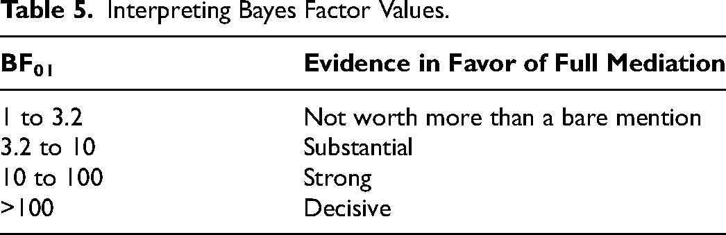
The magnitude of the Bayes factor is a measure of evidence. Kass and Raftery (1995) provide guidelines for how to interpret Bayes factors in terms of the amount of evidence supporting the model in the numerator of Equation 9, which in our case is the full mediation model (see Table 5). By symmetry of the Bayes factor, a value smaller than, for example, 1/100 would be decisive evidence against the model in the numerator, and therefore evidence for conditional dependence between X and Y in the data. However, because unobserved background variables (U_M,Y) confounding the causal relationship between M and Y will also result in conditional dependence, even in the presence of full mediation (see Table 3), small Bayes factors do not necessarily imply evidence against full mediation but simply fail to uniquely identify an underlying causal model. ¹⁵

Table 5.

Interpreting Bayes Factor Values.

BF01	Evidence in Favor of Full Mediation
1 to 3.2	Not worth more than a bare mention
3.2 to 10	Substantial
10 to 100	Strong
>100	Decisive

Violations of conditional independence can have multiple indistinguishable reasons, such that evidence supporting M₁ (β₃ ≠ 0) is inconclusive in the absence of prior knowledge about the data-generating causal structure. In contrast, evidence supporting M₀, in combination with a credible total effect (X → Y), reveals the data-generating causal model (i.e., [full] mediation) when X is randomly assigned. Next, we use an illustrative simulation to show how the Bayes factor can consistently measure evidence for the presence of a causal chain and, thus, for causal mediation. The simulation also shows how measurement error that is unaccounted for obscures the presence of a causal chain (i.e., the implied conditional independence relationship).

Illustrative simulation

We illustrate with simulated data from the model in Figure 4 with two indicator variables for M and Y each, and the following data-generating parameter values: X ∼ U(0, 1), β₁ = 1, β₂ = 3, β₃ = 0, {λ₁₀, λ₁₁} = {τ₁₀, τ₁₁} = {0, 1}, {λ₂₀, λ₂₁} = {1.5, 1}, {τ₂₀, τ₂₁} = {1.5, 1}, Var(U_M) = 1, Var(U_Y) = 1, $\mathrm{Var}({\mathrm{U}}_{{\mathrm{m}}_1^{*}})=.3$ , $\mathrm{Var}({\mathrm{U}}_{{\mathrm{m}}_2^{*}})=.6$ , $\mathrm{Var}({\mathrm{U}}_{{\mathrm{y}}_1^{*}})=.6$ , $\mathrm{Var}({\mathrm{U}}_{{\mathrm{y}}_2^{*}})=.3$ . We simulated and analyzed 1,000 data sets each for sample sizes N = 50, 200, and 1,000. Note that because β₃ = 0, we have a causal chain from X through M to Y that may, however, be obfuscated by the measurement error in indicators $({\mathrm{m}}_1^{*},{\mathrm{m}}_2^{*})$ of M. The purpose of the simulation is (1) to show how Bayes factors measure evidence supporting full mediation once we account for measurement error in the mediator and (2) to showcase consistency of the Bayes factor. The simulation also serves as a simple example of a power analysis for model choice.

Figure 5 summarizes the distribution of Bayes factors comparing the constrained model (β₃ = 0) with its unconstrained counterpart across simulated data sets. In Panel A, we report results from models that do not account for measurement error in the mediator and instead estimate the simple model using averages of the indicators $\{{\mathrm{m}}_1^{*},{\mathrm{m}}_2^{*}\}$ and $\{{\mathrm{y}}_1^{*},{\mathrm{y}}_2^{*}\}$ as direct composite measures of M and Y, respectively.

Figure 5.

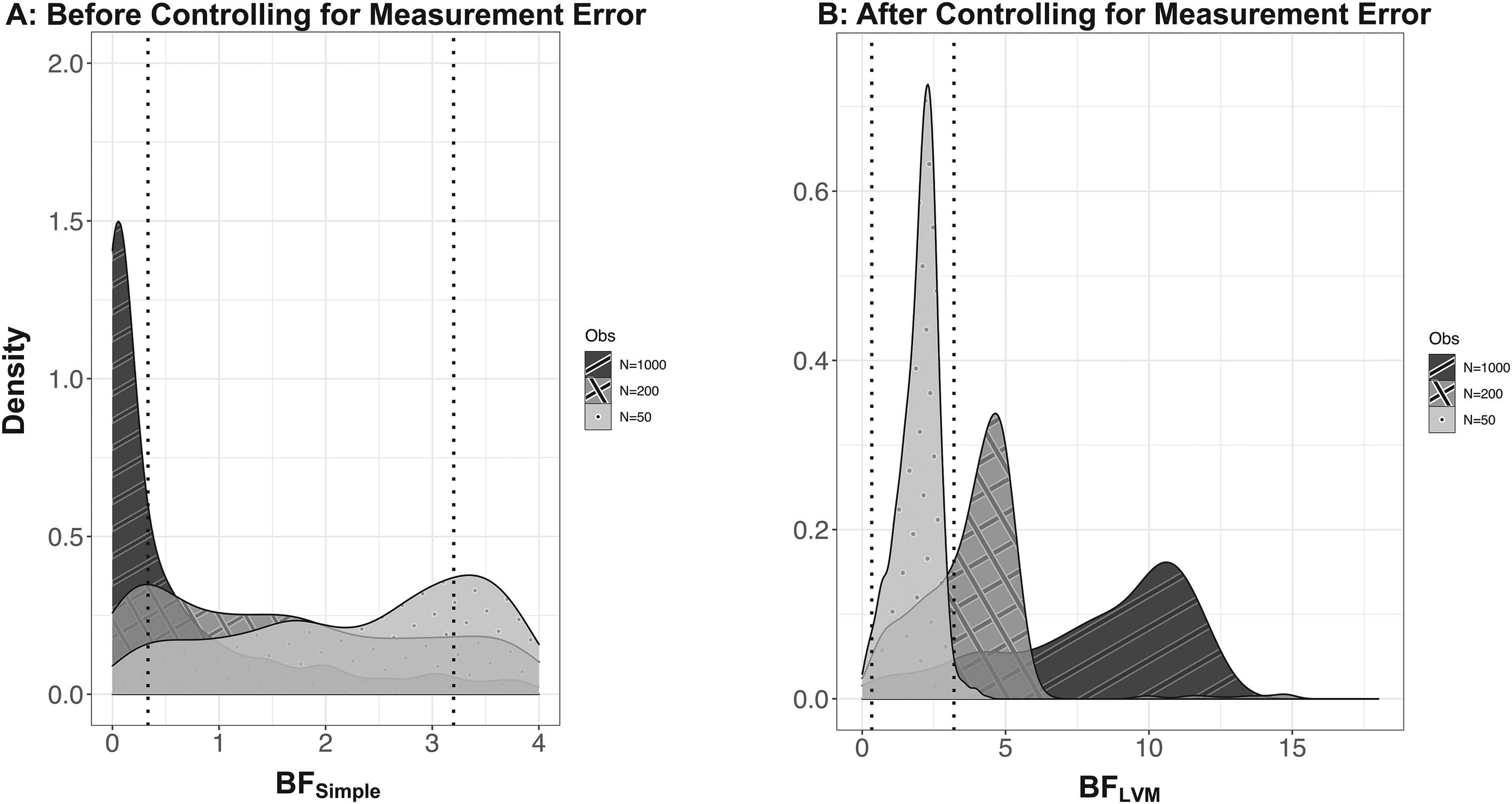
Bayes Factor Distribution Conditional on Different Sample Sizes in a Full Mediation Model Before and After Controlling for Measurement Error.

Figure 5, Panel B, summarizes results from models that do account for measurement error in the mediator (i.e., assess conditional independence between latent M and Y). In each panel, there are three distributions of Bayes factors (across simulated data sets), one each for the three sample sizes investigated. The dotted vertical lines in the figures demarcate the lower and upper end of the interval in which Bayes factors do not support a decision between models (see Table 5). However, we already note that it is best not to treat the border values .32 and 3.2 in Kass and Raftery's (1995, p. 777) guidelines as determinate thresholds that “just need to be cleared” for a decision, reminiscent of p-values. A Bayes factor of 3.2, for example, simply expresses that the model in the numerator is 3.2 times more likely than the model in the denominator, given the data and uniform priors over the two models. In addition, we strongly recommend adding more data in case of borderline results (see also Amrhein, Greenland, and McShane 2019). ¹⁶

When we do not account for measurement error, Bayes factors for N = 50 and N = 200 are spread out in the interval [0, 3.2], with N = 200 having more mass in [0, .32], which is the region with at least substantial evidence against the constraint β₃ = 0 (see Figure 5, Panel A). Larger data sets (N = 1,000), however, yield Bayes factors concentrated at very small values that translate into decisive evidence against β₃ = 0. Thus, we see how measurement error can obfuscate the causal structure that generated the data.

Once we control for measurement error using the LVM introduced in the “Measuring Evidence for Mediation” section, Bayes factors for N = 200 and 1,000 yield substantial evidence supporting the constraint β₃ = 0—that is, unequivocal support for the causal chain from X through (latent) M to (latent) Y (full causal mediation). It is noteworthy that the amount of evidence supporting the constraint increases in the sample size when the constraint holds, reflecting the symmetric consistency of the Bayes factor. This is a demonstration of how Bayes factors measure the amount of data-based evidence supporting a constraint. ¹⁷ When the data are less informative because of a small sample size (N = 50), Bayes factors do not support a firm decision between models, as they should given limited evidence.

Finally, the illustrative simulation reflects Rucker et al.’s (2011) observation that one is likely to spuriously reject conditional independence in the presence of measurement error. It also shows that testing conditional independence between latent M and Y is a viable strategy to overcome the complications from potential measurement error. Moreover, it illustrates how Bayes factors work as the sought-after metric of the degree of data-based support in favor of or against conditional independence given a model specification (cf. Preacher and Kelley 2011). In contrast, NHST fails to provide a measure of support for the null hypothesis by construction and thus cannot per se distinguish between an inconclusive result for a lack of power for detecting β₃ ≠ 0 and data-based evidence in favor of β₃ = 0.

The role of the subjective prior distribution

It is important to realize that a diffuse subjective prior for β₃ expresses not only a lack of prior knowledge about β₃ but also the firm belief that β₃ could be very large (in an absolute sense). Recalling that our target Bayes factor can be reexpressed as the ratio of the marginal posterior of β₃ over its subjective prior, both evaluated at zero, any concentration of posterior mass closer to zero will result in a Bayes factor supporting β₃ = 0 under a diffuse subjective prior. Put differently, a standard weakly informative diffuse prior for β₃ is only weakly informative given a fixed model structure, but highly informative in the context of model choice. It follows that for nontrivial model choice, we need to avoid diffuse priors for β₃.

In our simulations and in our reanalyses of published studies presented next, we use a normal prior for β₃ centered at zero and with prior variance equal to one (β₃ ∼ N(0, 1)). This setting has been advocated as a default or reference prior in psychology (see, e.g., Rouder et al. 2009, 2012; Wagenmakers et al. 2011). ¹⁸ This prior expresses that direct effects absolutely larger than two are outlying events (i.e., have a prior probability of less than 5%). However, it is important to recognize that the scaling of M and Y has implications for the scale of the direct and the indirect effect, which in turn has implications for model choice under any fixed prior distribution.

The following structural argument helps researchers recognize a potentially undue influence on model choice, from the combination of often arbitrary scaling and the advocated default priors here. Under the null hypothesis of full mediation, the indirect effect equals the total effect, and experimental data directly identify the total effect, as mentioned previously. If this effect is estimated as close to zero (very small in an absolute sense), the null hypothesis implies a direct effect estimate of the same order of magnitude. For example, if the total effect is only on the order of 10⁻³ or smaller, the default prior for β₃ advocated here may no longer be informative enough for nontrivial model choice. Conversely, if an experiment yields a total effect on the order of 10¹ or larger, the default prior choices for other parameters, and specifically those for variance terms, may no longer be uninformative, unduly influencing model choice.

In such cases, we recommend rescaling the Y variable for a total effect estimate in the order of 10⁻¹. Such rescaling—for example, multiplying Y by 10² (10⁻³) in case of total effects of order 10⁻³ (10²) on the original scale—renders the default prior for β₃ appropriately concentrated and those for other parameters uninformative for reliable model choice, as we show in a comprehensive simulation study discussed subsequently. As an alternative to the rescaling we recommend here, one could conduct a prior sensitivity analysis, as explained in the Web Appendix. ¹⁹

To be clear, the idea here is not to subjectively target the scale (or the subjective prior) of β₃ itself, which would be incoherent and defeat the purpose of measuring data-based evidence. The argument is, rather, to use the independently identified estimate of the total effect (which is equal to the indirect effect under the null hypothesis) to inform a reasonable choice. Moreover, we note that in the context of multiple indicators for latent M and Y, the default identification constraints described in the previous section automatically contribute to sensible scaling relative to our default priors. Finally, the reporting standards we suggest in the “Summary” section will automatically reveal undue strategic choices of subjective priors or scales that aim at producing a desired Bayes factor rather than measuring data-based evidence.

Comprehensive simulation study

To examine the robustness of the suggested procedure that combines latent variable modeling, Bayesian inference, and Bayesian model choice under different conditions that might arise in applied research, we conduct a simulation study. The simulation study investigates four different data-generating structures with binary treatment variables: (1) full mediation (see Figure 3), (2) partial mediation (see Figure 1), (3) structures with an unobserved M-Y confounder and no mediation (see Figure 2, Panel A), and (4) the case of a misspecified causal ordering of measured variables (see Figure 2, Panel B).

We investigate small (N = 50), medium-sized (N = 350), and large (N = 1,000) data sets. The medium sample size is roughly in line with the average sample size (N = 319) in the pool of published studies we reanalyze in the next section. Indirect and direct effect sizes are varied in a range following prior literature (Tofighi and Kelley 2020) and consistent with the range of estimated effects in our reanalysis of published studies. We vary the reliability of mediator and outcome indicator variables following Fritz, Kenny, and MacKinnon (2016). We include conditions with nonnormal error distributions following Finch, West, and MacKinnon (1997) and Tofighi and Kelley (2020). Finally, we vary the number of indicator variables mimicking the characteristics of published studies we reanalyze. In total, our simulation study features 3,024 cells. We base our results on 100 data replications in each cell, for a total of 302,400 data sets, MCMC runs, and Bayes factor computations.

Table 6 summarizes the simulation study in terms of Bayes factor accuracy across different data-generating structures and sample sizes, marginalizing over all other conditions in our simulation. The percentages displayed in Table 6 show, for each data-generating structure and sample size, how often the procedure at least substantially supports conditional independence where it should (first row), and how often it does not support conditional independence where it should not (all other rows). Confirming our previous discussion and illustration, smaller data sets (N = 50) do not contain enough information for Bayes factors to substantially support conditional independence. Reassuringly, we do not see false positives either (see the “N50” column in Table 6).

Table 6.

The Percentages of Bayes Factor Values in the Simulation Study Providing at Least Substantial Evidence for Conditional Independence (in the Full Mediation Model), Not Supporting Conditional Independence (in the Alternative Models).

	Sample
Model	N50	N350	N1,000
Full mediation	.2%	77.9%	89.4%
Partial mediation	99.9%	95.6%	99.9%
M-Y unobserved confounder	100%	98.8%	100%
M-Y misspecified direction	99.9%	99.9%	100%

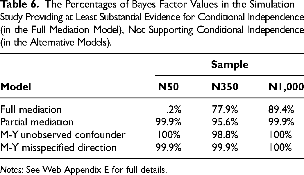
Notes: See Web Appendix E for full details.

In medium-sized data sets (N = 350), we find at least substantial evidence for causal mediation in roughly 80% of data sets generated from an unconfounded full mediation structure. The sensitivity increases to about 90% in large samples (N = 1,000). These results suggest N = 350 as a reasonable lower bound for studies aiming to potentially substantiate full causal mediation. ²⁰ Finally, when conditional independence is violated in the data-generating structure, Bayes factors reliably fail to support it (i.e., do not produce false positives; see Rows 2–4 of Table 6).

Table 7 provides a more detailed summary of results. The table presents coefficients from regressing the percentage of Bayes factors providing at least substantial evidence supporting (column “Full”), or refuting (all other columns) conditional independence on experimental factors of the simulation study. The columns correspond to the same four data-generating structures as described previously. The strength of indirect effect manipulation corresponds to the strength of the unobserved background connection between M and Y in Column 3 (“M-Y confounder”) and to the strength of the actual causal connection in Column 4 (“M-Y direction”), where the estimated model confuses the causal ordering of measured variables.

Table 7.

Results of the Regression.

	DV: % Substantial Evidence For/Against Conditional Independence
	Full	Partial	M-Y Confounder	M-Y Direction
	(1)	(2)	(3)	(4)
β1β2—Medium	−1.042**	−1.847	2.877**	2.285***
	(.437)	(1.127)	(1.189)	(.583)
β1β2—Large	−2.132***	−3.493***	5.516***	2.688***
	(.437)	(1.127)	(1.189)	(.583)
${\sigma }_{{\mathrm{m}}^{*}}^{}$	−.694*	−1.486	−1.650*	−3.199***
	(.357)	(.920)	(.971)	(.476)
${\sigma }_{{\mathrm{y}}^{*}}^{}$	1.472***	−1.745*	−7.171***	−.560
	(.357)	(.920)	(.971)	(.476)
N350	77.653***	55.899***	27.697***	64.674***
	(.437)	(1.127)	(1.189)	(.583)
N1,000	89.174***	75.646***	35.225***	67.424***
	(.437)	(1.127)	(1.189)	(.583)
${\mathrm{M}}_{\mathrm{in}{\mathrm{d}}_4}$	1.333***	5.588***	−.792	1.088**
	(.357)	(.920)	(.971)	(.476)
${\mathrm{Y}}_{\mathrm{in}{\mathrm{d}}_4}$	−.843**	.236	4.468***	3.116***
	(.357)	(.920)	(.971)	(.476)
Nonnormal1	.486	.816	.595	−.187
	(.437)	(1.127)	(1.189)	(.583)
Nonnormal2	.278	.771	.451	.639
	(.437)	(1.127)	(1.189)	(.583)
Constant	.398	23.028***	63.641***	30.546***
	(.592)	(1.526)	(1.610)	(.790)
Observations	432	864	1,296	432
R2	.992	.852	.455	.976

*p < .1. **p < .05. ***p < .01.

Notes: The dependent variable is the percentage of studies in the simulation study where the procedure correctly identifies (rejects) conditional independence in data sets generated from the full mediation model (alternative models). The (dichotomized) regressors are as follows: β₁β₂ = indirect effect (baseline = small effect), ${\sigma }_{{\mathrm{m}}^{*}}^{}$  = mediator measurement error variance (baseline = low variance, 1 = high variance), ${\sigma }_{{\mathrm{y}}^{*}}^{}$  = outcome measurement error variance (baseline = low variance, 1 = high variance), N = sample size (baseline N = 50), ${\mathrm{M}}_{\mathrm{in}{\mathrm{d}}_4}$  = 4 mediator multiple indicators (baseline = 2), ${\mathrm{Y}}_{\mathrm{in}{\mathrm{d}}_4}$  = 4 outcome multiple indicators (baseline = 2), nonnormal = measurement errors with nonnormal distributions (baseline = normal, 1 = moderately nonnormal, 2 = severely nonnormal).

The main result from our simulation is that sample size (N) is the key to measuring evidence supporting or refuting conditional independence. Other factors are either insignificant, despite 100 replications per simulation cell, or smaller in order of magnitude. More dependence between measured variables increases the chance of substantial evidence against conditional independence in Table 7, Columns 3 and 4. The smaller negative effect of the indirect effect strength on Bayes factor accuracy in full and partial mediation structures (Columns 1 and 2) is due to the induced correlation between X and M that translates into less statistical information about the direct effect. Larger measurement error variance ( ${\sigma }_{\mathrm{m}*},{\sigma }_{\mathrm{y}*}$ ) in general reduces Bayes factor accuracy. ²¹ More Y and M indicators (M_ind, Y_ind) in general lead to higher accuracy in Bayes factors. Finally, nonnormality of the error terms does not have a discernable effect on the assessment of conditional independence using our Bayes factor measure. Further details regarding our simulation study are available in the Web Appendix.

Reanalysis of Published Studies

To showcase the empirical relevance of the proposed methodology, we reanalyze five recently published mediation studies. ²² In the first two studies, NHST yields results only consistent with full mediation. We show how the proposed methodology, and specifically the application of Bayes factors, measures scaled evidence supporting full mediation (i.e., provides a metric). In the third study, the causal direction between the mediator and the outcome variable is uncertain. We demonstrate that the proposed procedure can determine the causal direction and thereby improves on the results from what is known as the “reverse mediation test” (Judd and Sadler 2003, pp. 129–30). The fourth study we discuss is an example of how measurement error results in biased estimates, obfuscating full mediation. We show how an LVM recovers evidence for conditional independence between Y and X given M, strongly confirming full mediation as the data-generating causal model. The fifth study yields results that are only consistent with mediation but do not identify the underlying causal model (like the simulated examples in the Web Appendix). Controlling for measurement error does not overcome the indeterminacy in this case. However, our analysis illustrates how controlling for measurement error yields an improved estimate of the indirect effect, if someone believes in (unconfounded) partial mediation as the data-generating causal model a priori. Finally, in the sixth study, we examine a serial mediation claim using our procedure and arrive at an explanation for the underlying process by ruling out equivalent models. This way, we are able to resolve fundamental uncertainties about the causal ordering of variables made explicit in the originally published analysis.

Empirical Illustration of Bayes Factors as Measures of Evidence Supporting Full Mediation

In the first study we reanalyze here, Shaddy and Fishbach (2017) show that customers ask for more compensation when a product is lost from a bundle than when it is lost in isolation. The reason, the authors argue, is that in the former case, in addition to the loss of the product, the “whole” of the bundle as a gestalt unit is compromised. Thus, the authors propose that the perceived need for replacement of the lost product mediates the effect of its loss from a bundle (vs. in isolation) on the amount of compensation demanded. In an experiment, participants were randomly assigned into two groups imagining that they have purchased three suitcases either as a bundle or separately (X). The participants were then asked how much, in dollars, they think they should be compensated (Y), and how important, on a seven-point rating scale, it would be to replace the missing item (M). The authors estimate a significant indirect and an insignificant direct effect (see Figure 6, Panel A, and Table 8).

Figure 6.

Mediation Diagrams with Standard Test Results.

Table 8.

A Comparison of NHST, Direct Effect Bootstrapped Confidence Interval, and Bayes Factor in Cases Where Full Mediation Hypothesis Cannot Be Rejected Based on NHST.

	Shaddy and Fishbach (2017)	Yan and Muthukrishnan (2014)
Sample size	200	91
NHST	Fail to reject full mediation	Fail to reject full mediation
Direct effect bootstrapped CI	[−.29, .05]	[−1.33, .09]
Bayes factor	4.9	.66

While these results are consistent with full mediation, it is hard to tell how much evidence they provide. For example, the asymmetry in the bootstrapped 95% confidence interval may lead to speculations about a lack of statistical information about the direct effect in the data. The Bayes factor we compute for this study points to substantial evidence supporting full mediation (BF = 4.9), alleviating this and similar concerns.

Substantively, evidence supporting full mediation, among other competing explanations, rules out a reverse causal direction from demanding a high compensation amount (Y) to reporting a high perceived importance of replacement (M). This is particularly helpful in this study because the perceived importance of replacement was elicited only after asking for the compensation amount. Without the data-based insight into the causal ordering from X via perceived importance of replacement to the compensation amount, the time order of measurements could lead to speculations about a different process.

The second study we reanalyze here, by Yan and Muthukrishnan (2014), proposes that consumers’ valuations of a lottery-based promotion and intentions to participate in such a promotion are greater when the lottery excludes (vs. includes) consolation prizes. The authors hypothesize that the effect of the consolation prize (X) on participation intention (Y) is mediated by the perceived likelihood of winning (M). The authors report qualitatively similar estimation results as in the study by Shaddy and Fishbach (2017) discussed previously, based on which they claim full mediation (see Figure 6, Panel B, and Table 8). Even though the NHST results are consistent with full mediation ( $95\text{\%}\mathrm{C}{\mathrm{I}}_{{\beta }_3}=[-1.33,.09]$ ), the Bayes factor we compute reveals a lack of evidence for full mediation (BF = .66). There is just not enough information in the data to rule out alternative models, and precisely this lack of information could have caused the insignificant direct effect estimate. As such, this study does not per se deliver data-based evidence for mediation. The causal process interpretation of what could be an indirect effect has to rest on subjective prior assumptions about the underlying data-generating model structure. ²³

The small sample size of this study plays a crucial role in the inconclusive Bayes factor results. Collecting more data to be added to the original sample and recomputing the Bayes factor would be the natural next steps toward a decision about the underlying causal model. We provide additional recommendations regarding sample size and other aspects of measurement-of-mediation designs in the “Summary” section.

Determining the Causal Direction

Mazar and Aggarwal (2011) investigate whether the effect of collectivism (vs. individualism) on the propensity to giving bribes is mediated by the degree of perceived responsibility of the individual (Figure 7, Panel A). Mazar and Aggarwal randomly assigned individuals into collectivist and individualist groups (X) using different priming tasks. Individuals then had to decide whether they would bribe an international business partner or not (Y) and subsequently indicated their degree of perceived responsibility (M). The authors find a significant indirect effect of collectivism on the propensity to bribe.

Figure 7.

Original Mediation Hypothesis by Mazar and Aggarwal (2011) and the Reverse Model.

However, Mazar and Aggarwal (2011) express uncertainty about the roles of perceived responsibility and propensity to bribe. To argue against perceived responsibility as a “post hoc realization consequent to the decision to bribe” (p. 845) and confirm their original hypothesis, they run a reverse mediation test by comparing the indirect effect estimate from the originally hypothesized model (Figure 7, Panel A) with that from the model where the decision to bribe is the mediator and perceived responsibility is the dependent variable (Figure 7, Panel B). Table 9 shows the indirect effect estimates from the two models. Both effects are significant, and the indirect effect implied by the reverse model is considerably larger in magnitude. ²⁴ In addition, the direct effects under both model specifications are consistent with full mediation and cannot be reliably distinguished from zero based on p-values. ²⁵

Table 9.

A Comparison of the Results of the Reverse Mediation Test and the Bayes Factor.

	Hypothesized Direction	Reverse Direction
Indirect effect (reverse mediation test)	−.096*	−.228*
Direct effect	−.09	−.36
Bayes factor	6.66	1.17

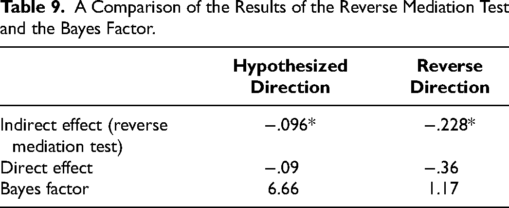
We estimated the simple mediation model with the causal direction first pursued by Mazar and Aggarwal (2011). The corresponding Bayes factor is 6.66, supporting a causal chain from X (collectivist vs. individualist) through M (perceived responsibility) to Y (the decision to bribe) as depicted in Figure 3, essentially ruling out an alternative ordering of variables as well as unobserved background variables influencing both M and Y. We then reversed the order of the mediator and the dependent variable in the model and obtained a Bayes factor of only 1.17. The smaller Bayes factor is equivocal regarding the absence or presence of conditional independence and thus fails to support the reverse causal direction (as it should, given the large value from earlier). Based on these results, and in fact already based on the first Bayes factor computed here, we have data-based evidence uniquely identifying the causal chain from X (collectivist vs. individualist) through M (perceived responsibility) to Y (the decision to bribe) in this study.

Testing Full Mediation Accounting for Measurement Error

Small Bayes factor values indicate that there is insufficient empirical evidence to pinpoint an underlying model. Very small Bayes factors are evidence against conditional independence and, hence, prima facie evidence against full mediation. However, since measurement error and discretization might confound testing conditional independence between Y and X given M, controlling for these aspects of measurement may still establish full mediation as the causal model generating the data in these instances. Controlling for these two sources of bias is possible when a study features multiple indicators for measured variables. Next, we showcase how this can improve mediation analysis in an empirical example.

Sussman and O’Brien (2016) assess whether people take on average a smaller amount of money from the savings they have set aside for their children, education, or retirement (vs. taking a vacation or buying a car), because they perceive doing so as irresponsible (e.g., “Taking money from savings that was set aside [for my child] makes me feel like a bad person”). They use bootstrapping to statistically test what could be an indirect effect and find results consistent with mediation. As we have previously discussed, this result in isolation is equivocal (i.e., does not identify mediation as the underlying causal model). For example, it seems hard to rule out a priori that respondents answer the questions about the perceived irresponsibility of their withdrawals at least partly in reaction to the amount of money they said they would take from a particular savings account. Again, the order of measurements that first elicits the withdrawal amount and then asks about the perceived irresponsibility may contribute to such a relationship.

Estimating a simple mediation model, we find that the 95% posterior credible interval (PCI) yields a barely insignificant direct effect ( $95\text{\%}\mathrm{PC}{\mathrm{I}}_{{\beta }_3\mathrm{simple}}=[-.02,.33]$ ). ²⁶ A Bayes factor of 2.1 indicates a negligible amount of evidence supporting full mediation from savings account type (X) through perceived responsibility (M) to the withdrawal amount (Y). This leaves room for alternative interpretations.

In search of more accuracy and potentially conclusive results that rule out alternative causal models, we leverage the multiple measures of perceived responsibility in this study. Perceived responsibility is measured using three questions on seven-point rating scales. Using these measures as indicators, we calibrate an LVM to investigate the possibility that measurement error and discretization may have affected the results (Figure 8). In contrast, the simple model uses the average of the responses to these questions as a composite measure of the mediator.

Figure 8.

Diagram of Sussman and O’Brien’s (2016) Mediation Study.

Figure 9, Panel A, illustrates the posterior distribution of the indirect effect through perceived responsibility. Panel B shows the posterior distribution of the direct effect. Both panels overlay the respective posteriors from the simple model and the LVM. Comparing posterior distributions between the two models reveals that after accounting for discretization and measurement error, the indirect effect PCI increases from [.12, .32] in the simple model to [.20, .47] in the LVM (see Panel A). In addition, the direct effect estimate, which barely covered zero before accounting for measurement error and discretization, now is closer to zero, and its PCI almost symmetrically straddles zero ( $95\text{\%}\mathrm{PC}{\mathrm{I}}_{{\beta }_3\mathrm{LVM}}=[-.14,.24]$ ). In line with these observations, the overall evidence uniquely supporting full mediation as the underlying causal model has increased to substantially support this model (BF = 8.5). The result is useful because it rules out alternative causal models that may be altogether inconsistent with mediation.

Figure 9.

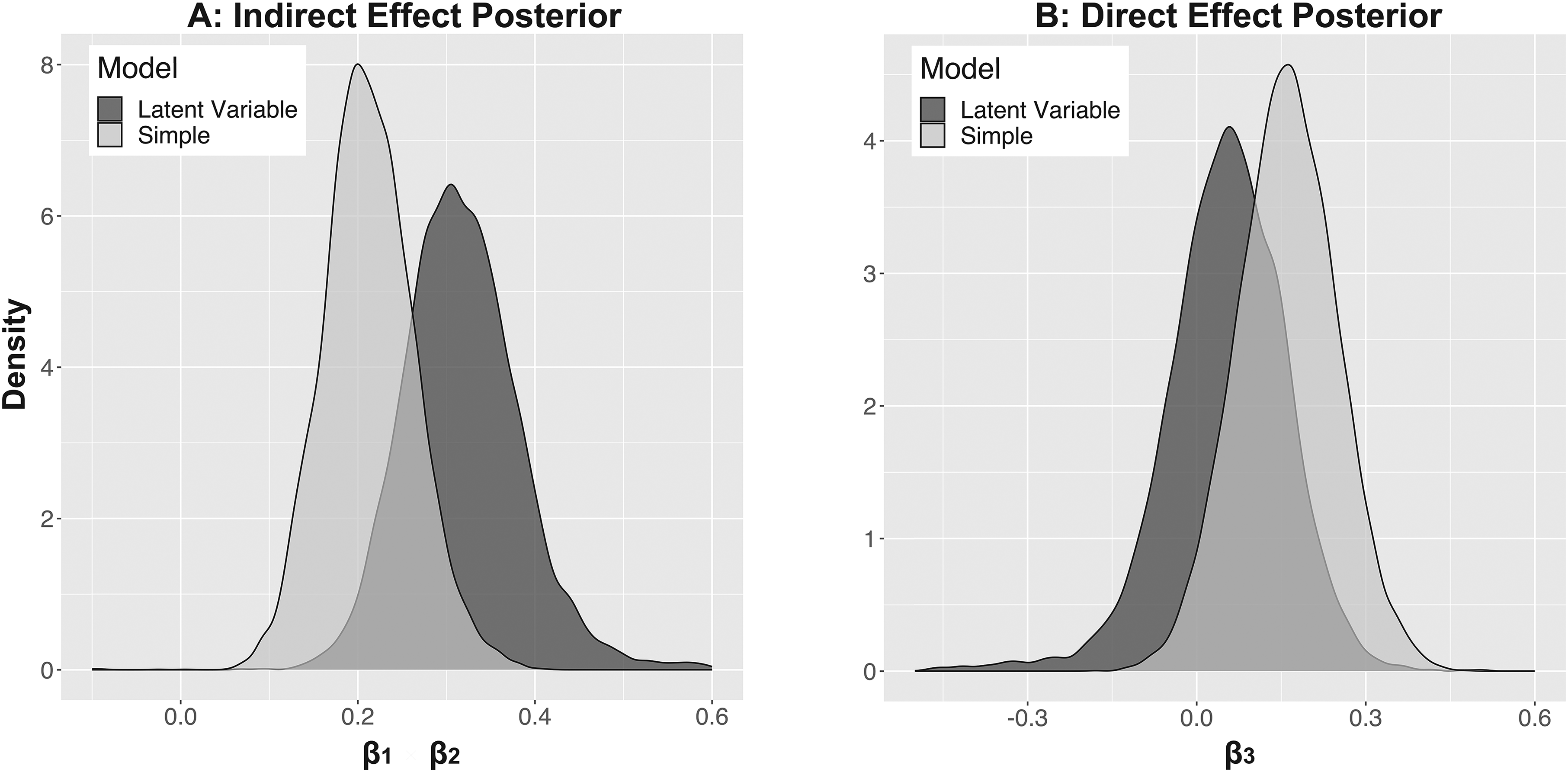
Overlay Plots of the Indirect Effect and the Direct Effect Posterior from the Reanalysis of the Mediation Study in Sussman and O’Brien (2016).

Assessing (Potential) Partial Mediation in the Presence of Measurement Error

If a data set is generated by a partial mediation model, or common unobserved causes link M to Y, Bayes factors will reject conditional independence between Y and X given M and thus fail to produce evidence supporting full mediation, as they should, even after controlling for measurement error. An empirical example can be found in Sela and LeBoeuf (2017). These authors hypothesize that people are more likely to buy an upgrade of the product they own if they are not encouraged to compare the upgrade with the status quo product, and this happens because they tend to perceive the upgrade as more dissimilar to their current version.

Sela and LeBoeuf (2017) conducted an experiment in which they randomly assigned participants to the treatment group, where participants were prompted to compare their current mobile phone with an upgraded version of the phone (X). All participants were then asked to rate the similarity of their phone with the upgrade version (M), using two questions on seven-point rating scales, and rate how interested they would be to upgrade their phone (Y), again on a seven-point scale. Statistics reported in the paper, based on bootstrapping, suggest a significant indirect effect, based on which the authors concluded that mediation is present ( $95\text{\%}\mathrm{C}{\mathrm{I}}_{{\beta }_1\times {\beta }_2}=[-.36,-.06]$ ).

We use the two (ordinal) indicators of perceived similarity (M) in an LVM. Even after controlling for measurement error and discretization of mediator measures, the Bayes factor decisively rejects conditional independence between the experimental condition and the purchase intention after controlling for similarity (BF = .000006). However, if there is a strong prior belief that partial mediation (see Figure 1) is the underlying causal model, the 95% PCI of β₁ × β₂ from this model is the preferred estimate of the indirect effect because measurement error and discretization of observed measures are controlled for. In fact, the estimate is more reliably negative than that from the simple model ( $95\text{\%}\mathrm{PC}{\mathrm{I}}_{{\beta }_1\times {\beta }_2\mathrm{LVM}}=[-.42,-.08]$ ).

This study presents a case where evidence from the data is insufficient to identify the data-generating causal model. However, accounting for sources of bias, namely measurement error and discretization, can yield cleaner, more reliable parameter estimates in a partial mediation model, which we may believe to be true a priori.

Testing Serial Mediation

In the last exemplary study we reanalyze, Tonietto and Malkoc (2016) use NHST to obtain results consistent with serial mediation. The results suggest that scheduling a leisure activity (X) makes it feel less free-flowing (M1), which in turn makes that activity feel more like work (M2), which finally reduces participants’ anticipation utility (Y) (see Figure 10, Panel A). However, the authors note that such a mediation model cannot establish a causal ordering of variables, and they mention that anticipation utility could be an antecedent to work construal, or that anticipation utility and work construal could be joint dependent variables rather than sequential outcomes of scheduling.

Figure 10.

Mediation Diagrams of Tonietto and Malkoc (2016).

We next show how our suggested approach applies to testing serial mediation and thereby helps rule out some of the alternative interpretations mentioned by Tonietto and Malkoc (2016). For an empirically validated causal interpretation of conditional effects connecting measured variables M1 to M2 and M2 to Y as causes and consequences, we need (1) conditional independence between X and M2 given M1 (X → M1 → M2), (2) conditional independence between X and Y given M1 (X → M1 → Y), and (3) conditional independence between X and Y given M2 (X → M2 → Y). ²⁷ Conditional independence Relationship 1 establishes the indirect effect from X to M2 via M1 as the only causal connection between X and M2 and, thus, that the effect from M1 to M2 is causal. Relationship 2 establishes the indirect effect from X to Y via M1 as causal, eliminating the possibility of a direct effect or unobserved noncausal connections between M1 and Y. Relationship 3 establishes the indirect effect from X to Y via M2 (again eliminating the possibility of a direct effect and of unobserved noncausal connections between M2 and Y). Together, these conditional independence relationships uniquely establish the causal chain from X (scheduling a leisure activity) via M1 (a less free-flowing experience) to M2 (work construal) and finally to Y (anticipation utility). Conditional independence between M1 and Y given M2 (M1 $\to$ M2 $\to$ Y) is implied. ²⁸

The Bayes factors comparing the respective models assuming conditional independence to their dependent alternatives are (1) 2.3, (2) 12.1, and (3) 12.9. Thus, the results strongly support the causal models X → M1 → Y and X → M2 → Y but fail to support X → M1 → M2. In addition, testing conditional independence between M1 and Y given M2 (M1 → M2 → Y) yields a Bayes factor of only .02, strongly rejecting conditional independence and, thus, the unique identification of the serial causal chain X → M1 → M2 → Y as the data-generating model. In fact, our results rule out all causal models that feature X, M1, M2, and Y as four conceptually distinct variables. Specifically, the strong support for conditional independence between X and Y given either M1 or M2, coupled with the failure to support additional independence relationships, is at odds with any causal ordering of these four variables.

However, from the strongly supported conditional independence implied by X → M1 → Y and by X → M2 → Y, we learn that the triples {X, M1, Y} and {X, M2, Y} each individually consist of conceptually different variables. The possibility of a causal ordering only vanishes when we consider M1 and M2 as conceptually different. Thus, we investigated a model that uses the indicators of M1 and M2 as measures of one latent mediator M (see Figure 10, Panel B) and again obtain strong support for conditional independence as implied by the model X → M(M1, M2) → Y, with a Bayes factor of 11.9.

Compared with Tonietto and Malkoc's (2016) original conclusion, we strongly establish anticipation utility (Y) as a conceptually distinct final outcome. We also conclusively establish mediation by M1 (M2) as the causal transmission mechanism from scheduling a leisure activity or not (X) onto anticipation utility (Y). However, at the same time, our results strongly refute the possibility of a causal ordering among M1 and M2 and, thus, serial mediation. Together with conditional independence between X and Y given either M1 or M2, it follows that M1 and M2 are not conceptually distinct in their relation to X and Y.

The proposed procedure combines Bayes factors with LVMs to identify causal mediation in the data by examining conditional independence. The results point to the importance of each of the procedure's components as well as the procedure as a whole. The data from Yan and Muthukrishnan (2014) and Shaddy and Fishbach (2017) showcase empirically how the suggested Bayes factor provides a metric of support for full causal mediation—that is, distinguishes between an insignificant direct effect resulting from a lack of power or sample variability, as in Yan and Muthukrishnan, and strong data-based support for conditional independence, as in Shaddy and Fishbach. The reanalysis of Mazar and Aggarwal (2011) demonstrates that data-based support for conditional independence reflected in the Bayes factor can resolve potential uncertainties about the causal direction between measured variables. The fourth application from Sussman and O’Brien (2016) provides an empirical example for obfuscation from measurement error and showcases our ability to measure support for conditional independence between X and Y given latent M. The fifth application from Sela and LeBoeuf (2017) exemplifies a case in which our procedure results in evidence against conditional independence, even after controlling for measurement error. In such cases, as previously summarized in Table 3, ambiguity about the underlying causal model cannot be resolved. However, if prior knowledge rules out unobserved confounders as well as a reversed Y → M causal ordering, the estimated indirect effect can be interpreted as causal. ²⁹ Finally, the last application shows how the procedure can help resolve uncertainty about the causal ordering and nature of variables under investigation. We reduce several prior possible causal structures suggested in Tonietto and Malkoc (2016) to only one, which derives from the conditional independence relations we find in the data. This way, our approach helps researchers elucidate the causal structure underlying their data as compared with focusing on functions of coefficients in a given model of serial mediation (e.g., Tofighi and Kelley 2020).

The Web Appendix summarizes the results from the reanalysis of all the studies we surveyed, along with bootstrapped parameter estimates, following Preacher and Hayes (2004). There, we again see that bootstrapped direct effects can mislead the analyst into claiming full mediation in cases where insignificant direct effects result from small samples or otherwise uninformative data, and that measurement error and discretization can obfuscate the presence of an unconfounded causal chain and, thus, full mediation at the causal theory level.

Summary

Figure 11 summarizes the proposed approach toward mediation analysis. What makes the approach useful and novel is that it presents a unified and computationally reliable Bayesian framework for the modeling of measurement error in, and the discretization of observed indicators integrated with, the assessment of conditional independence between (latent) Y and X given (latent) M. It applies in settings where X is randomly assigned and M and Y are measured (measurement-of-mediation designs).

Figure 11.

A Flowchart of the Proposed Method for Mediation Analysis.

Assuming a statistically reliable total effect (X → Y), all paths in the flowchart, in which conditional independence is firmly established, unequivocally identify the causal chain from X through M to Y—and, thus, full causal mediation—as the underlying data-generating mechanism. Paths that terminate inconclusively point to situations where claims about mediation rest on subjective prior assumptions about the underlying data-generating mechanism (see also Table 3). ³⁰

Next, we explain the procedure step-wise. Computer code with examples is available at GitHub, and a web application with a graphical user interface is available at Shinyapps.io (for a tutorial guide, see the Web Appendix).

Estimate the simple mediation model.

Compute the Bayes factor (Equation 9) in the simple model.

If the Bayes factor strongly supports full mediation (BF > 3.2), proceed to Step 6; otherwise, proceed to Step 4.

Estimate the LVM with multiple indicators.

Compute the Bayes factor in the LVM.

Report point estimates and the Bayesian 95% PCI of the indirect and direct effect, as well as the Bayes factor and the subjective prior settings.

Note that in Step 4, the minimum number of indicators to achieve identification is two for each latent variable (see the Web Appendix). ³¹ We recommend using the reference prior for the direct effect and interpreting the Bayes factors based on Kass and Raftery’s (1995) guidelines (see Table 5).

Our simulation study illustrates the robustness of the suggested approach across a wide and empirically relevant range of possible data-generating mechanisms and estimation specifications. However, some care is in order when an experiment yields a total effect of 10⁻³ or smaller. With such small effects, the default prior for β₃ may no longer be informative enough for nontrivial model choice in all but very large samples. Conversely, if an experiment yields a total effect of 10¹ or larger, our default priors for other parameters may no longer be uninformative. In both cases, we recommend rescaling Y for a total effect estimate of 10⁻¹. However, we note that reasonable scaling is essentially automatic in the preferred situation with multiple indicators for (latent) M and (latent) Y.

Keeping with the reporting standards suggested in the step-wise description will automatically reveal undue strategic choices of subjective priors or scales that aim at producing a desired Bayes factor rather than measuring data-based evidence. Moreover, we advise against making overconfident claims in favor of or against conditional independence based on Bayes factors marginally larger than 3.2 or smaller than .32, and we generally recommend sample sizes of N = 350 or larger in the search for the underlying causal structure in measurement-of-mediation designs. If the Bayes factor value is within the [.32, 3.2] interval or near the boundary values, we recommend collecting additional data. The Bayesian paradigm allows, and in fact strongly encourages, the researcher to simply add new observations to an existing data set in search for more data-based evidence, rather than independently analyzing a fresh draw. This usefully limits researchers’ degrees of freedom from capitalizing on chance. ³²

As we have shown, measurement error and discretization may obfuscate evidence in favor of full mediation. Therefore, estimating an LVM using multiple indicators for measured variables may reveal full mediation at the causal theory level. To help researchers prior to collecting (additional) data, we offer a simulation-based Bayesian power analysis as part of the R package accompanying this paper.

Strong evidence for conditional independence between Y and X given M in the simple model rules out all other possibilities but the causal chain from X through M to Y. In this case, as instructed in Step 3 of the procedure, we can immediately, confidently claim full mediation as the causal model generating the data (assuming evidence supporting total effect α ≠ 0). The unified integration of latent variable modeling, MCMC estimation, and Bayesian model comparisons facilitated by the latter enables researchers to harness the unique mapping from evidence for conditional independence between X and (latent) Y given (latent) M into evidence for mediation as the data-generating causal model, even in the presence of measurement error.

We conclude by discussing potential extensions to our suggested procedure. First, our reanalysis of the study by Tonietto and Malkoc (2016) shows how to leverage our suggested approach in the context of potential serial mediation. Similarly, we can use the suggested approach to obtain potentially conclusive results in the context of parallel mediation, in a causal sense. Evidence for parallel mediation as the underlying causal model results from conditional independence between X and Y given a set of mediators M = {M₁, M₂, …}, where omitting any element from the set leaves X and Y conditionally dependent.

Second, when X changes not only the level of M but also how M transmits its causal effect to Y, sometimes referred to as a case of “moderated mediation” (see, e.g., Judd and Kenny 1981; Preacher, Rucker, and Hayes 2007), even controlling M by experimental means does not shield Y from X. In this model, a specific, fixed M translates into a different Y depending on X. Thus, establishing conditional independence between X and Y given M also rules out X as a moderator of the effect from M to Y, and more generally X as a conditioning argument to any causal consequences of M (that is not exactly mean preserving). While it is possible to extend our measure of data-based evidence for β₃ = 0 to this case of moderated mediation, the lack of a direct effect in this model does not follow from a conditional independence relationship in the causal model. Finally, the generalization of our procedure to the more common case of manipulated third variable(s) Z, moderating the effects between X and M (as in PROCESS Model 7) or that between M and Y (as in PROCESS Model 14), or both (as in PROCESS Model 21) involves testing for conditional independence under all levels of the moderating variable(s) (for the definitions of different PROCESS models, see Hayes [2022]).

This article is accompanied by computer code in package form (available at GitHub) that runs under R (R Core Team 2020). The examples included in the package illustrate how to assess sensitivity with respect to subjective prior assumptions, conduct a Bayes factor power analysis prior to data collection, and assess the convergence and MCMC stability of decision-relevant quantities such as the Bayes factor. The package includes three of the data sets reanalyzed in the “Reanalysis of Published Studies” section and a web application available at Shinyapps.io. Finally, the Web Appendix offers step-wise instructions to replicate selected reanalyses.

Supplemental Material

sj-pdf-1-mrj-10.1177_00222437231151873 - Supplemental material for Measuring Evidence for Mediation in the Presence of Measurement Error

Supplemental material, sj-pdf-1-mrj-10.1177_00222437231151873 for Measuring Evidence for Mediation in the Presence of Measurement Error by Arash Laghaie and Thomas Otter in Journal of Marketing Research