Omitted Budget Constraint Bias and Implications for Competitive Pricing

Abstract

Standard choice-based conjoint models often ignore or insufficiently approximate consumers’ budget constraints, despite the prominent role of budget constraints in economic theory. The authors offer a theoretically motivated improvement to the choice-based conjoint model that is especially appropriate for high-ticket durable goods and develop a Bayesian method for the inference of unobserved budget constraints. The proposed method leverages respondents’ stated budget constraints that suffer from measurement error and respondents’ financial demographic variables as additional information to reduce the dependency on functional form assumptions in the estimation. The authors show that accounting for budget constraints substantially increases model fit and the accuracy of competitive pricing in an industry-grade discrete-choice experiment on consumer preferences for high-end laptops. The proposed model performs better than the canonical linear price benchmark model, which is not flexible enough to approximate budget constraints. In theory, more flexible utility specifications, such as the nonlinear dummy price model, can approximate consumers’ budget constraints. However, they perform poorly when only finite data are available. The authors conclude that applied researchers in industry and academia will benefit from having a better tool for estimating budgets in high-ticket categories.

Choice-based conjoint (CBC) is among the most widely used quantitative research methods to determine profit-maximizing product attributes and optimal prices (e.g., Hauser, Eggers, and Selove 2019; Orme 2020), used in about 20,000 applications per year. Larger firms (such as General Motors) spend tens of millions of dollars annually using CBC analysis to design optimal products (Hauser, Eggers, and Selove 2019). The diffusion of concepts from industrial organization into marketing and the advancement of computational methods have further broadened the scope of market outcomes that can be investigated using CBC. For example, Allenby et al. (2014a, b) propose a method for quantifying the market value of patents and copyrights that builds on the inference of market equilibrium prices that take competitive reactions into account.

A driver of this development is the prominent role of CBC methods in recent lawsuits. Expert witnesses rely on inference from CBC to assess damages in the context of alleged patent infringements (e.g., Sidak and Skog 2016). For example, inference from CBC played a role in Apple v. Samsung (2017), in which Apple sued Samsung in 2011 over patent infringements. Expert witnesses on Apple's side based their assessment of the market value of the corresponding product features on an inference from CBC. The argument convinced the court to rule that Samsung had to pay Apple about 1 billion USD in damages.

Although many large-stakes decisions have been made using CBC-based inference, the economic assumptions implied by standard CBC models may not apply for high-ticket durable goods, such as laptops, smartphones, or cars. Standard CBC models typically ignore or insufficiently approximate consumers’ budget constraints despite the prominent role of budgetary constraints in economic theory (see, e.g., Deaton and Muellbauer 1980). To fill this gap, we develop a Bayesian methodology for the inference of latent budget constraints in CBC surveys. We show how adding this theoretically motivated improvement facilitates the use of CBC for high-ticket durable goods.

Leveraging the survey nature of CBC experiments, we ask respondents about relevant financial indicators that help identify unobserved budget constraints in estimation. First, we build on insights from household finance theory that relate constraints on spending for consumption to available financial resources (e.g., Deaton 1991). In our empirical study, we elicit disposable income (taking fixed monthly expenditure commitments into account) and the value of liquid assets as theory-based determinants of budget constraints. We introduce these financial demographic variables as conditioning arguments of unobserved heterogeneity, adding to our model a theory-based source of information about latent budgets.

Second, we ask respondents to state their budgets after they learn about the specific attributes and levels included in the experiment, excluding price. ¹ The stated budgets provide valuable information but suffer from measurement error. Moreover, it is generally difficult for respondents to differentiate “expenditure goals” from “expenditure caps” in surveys, which leads to an underreporting of budgets (Moore, Stinson, and Welniak 2000). It is also known that consumers tend to underestimate their spending on exceptional durable good purchases (Sussman and Alter 2012). To address this circumstance, our proposed model incorporates stated budgets as fallible indicators of unobserved budgets in the individual-level likelihood functions. The measurement error model penalizes large deviations between stated and unobserved budgets in the likelihood function and thus mitigates the problem of extrapolating to extremely large budgets based on subjective distributional assumptions.

We emphasize that the proposed approach relies on eliciting both causal parents of budgets (e.g., disposable income) and a potentially direct measure (e.g., stated budget). The inferred relations between these variables and model parameters empirically support our claim that we account for consumers’ budget restrictions. Only the combination of causal parents and the potentially direct measure translates into an unequivocal interpretation of the inferred screening rule and confidence in its stability. Importantly, relating the potentially direct measure to its causal parents allows for an assessment of these measures based on theory, and before fitting the choice model.

We show that omitting the budget constraint, as in the standard discrete-choice framework, substantially biases inferred optimal actions and counterfactual market outcomes in an industry-grade CBC experiment on high-end laptops. The proposed methodology accounts for budget constraints in estimation and market simulation, substantially improving inference in the context of competitive price optimization. For example, we find that the standard linear price model overstates the equilibrium price for the premium brand Dell by 20.65%, even after removing information-poor respondents (Allenby et al. 2014a). ² As indicated by these results, our model offers a solution that has the potential to significantly increase the use of inference from CBC in marketing decisions in high-ticket product categories. Our application methodology is parsimonious and general because it effectively reduces to the canonical linear price model if all individuals have sufficient budget to afford even the largest price in an application.

In our empirical analysis, we also estimate the choice model that infers respondents’ budget constraints purely from choice data without accounting for stated budgets in the likelihood function. We find that the implied posterior budget distribution resembles the budget distribution if the estimation accounts for stated budgets, indicating convergent validity. However, accounting for respondents’ stated budgets is valuable for disciplining the tails of the inferred budget distribution, as the choice data convey little information if respondents’ budgets are sufficiently large relative to the price support in a CBC study.

Integrating consumers’ budget constraints into the standard CBC framework requires a careful specification of the experimental design. First, price ranges must be wide enough to cover a substantial part of the unobserved budget distribution. Hence, we include prices as high as 4,000 EUR for a laptop in our empirical case study. However, including much higher prices results in a loss of statistical design efficiency when prices vary independently of other attributes. For example, not choosing weak alternatives at high prices is not informative about budgets and conveys little information about other model parameters. Thus, we introduce dependencies between prices and attribute levels in our design. Specifically, our design never combines the strongest (weakest) attribute levels with the lowest (highest) price for the memory, screen size, processor, and hard disk size attributes. ³ Second, we show that including respondents’ stated budgets and financial demographic variables in the model aids empirical identification of budget constraints and substantiates their interpretation. We propose that these variables should be routinely included in CBC studies investigating demand in high-ticket categories.

The remainder of the article is organized as follows. First, we discuss related concepts that have been suggested in the literature for improving inferences of optimal prices in CBC studies. We then develop the Bayesian methodology for the inference of budgets and provide identification arguments. Next, we show that benchmark methods do not sufficiently account for unobserved budgets using simulated data. We then showcase an empirical application using data from a large discrete-choice experiment in the high-end laptop category. Finally, we offer concluding remarks.

Related Literature

The problem of inferring unrealistically high prices from CBC optimization exercises is widely known among applied researchers. As we propose to account for unobserved budget constraints to improve competitive price optimization, our work is related to other remedies in the literature that aim to address either data quality issues or functional form misspecification in the utility model.

Existing approaches to improve inference for optimal prices from CBC focus on respondents’ motivation. In incentive-aligned choice experiments, researchers endow respondents with a real monetary budget that needs to be spent as a function of choices in the experiment made by the respondent (e.g., Ding 2007; Ding, Grewal, and Liechty 2005). In the context of higher-ticket items, the required endowments can make experiments prohibitively expensive (e.g., Ben-Akiva, McFadden, and Train 2019). For example, endowing 100%, 50%, or 10% of 1,000 respondents in our empirical CBC study with the maximum included price for a laptop would have added approximate costs of 4 million, 2 million, or 400,000 EUR. The solution of offering only a chance to win the endowment is useful, but with limitations because small chances may dilute the incentive (Yang, Toubia, and De Jong 2018).

However, even when the stakes are high enough for the decision maker to want to offer large endowments to all respondents, the very size of the endowment can make respondents systematically depart from what they would do in the market with their own money, without the endowment. For example, the endowment of 4,000 EUR for a high-end laptop may change the choice between inside goods due to income effects.

To validate these considerations, we surveyed market research industry practitioners and asked about the use of incentive-aligned conjoint methods at the institutions they work for. ⁴ We received answers from practitioners representing 34 different international market research companies, who reported that a total of 613 conjoint studies had been conducted at their institutions in the past 12 months. Of those 613 studies, the vast majority (about 96%) were conducted without incentive alignment. The most commonly stated reasons were that incentive-aligned experiments would be “too expensive” and result in “too high administration costs.” In addition, many practitioners stated that they were “not convinced that incentive-aligned methods pay out” and that delivering chosen products to participants after the survey would be a “logistic nightmare.” Accordingly, our research aims to improve inference in higher-ticket items, where incentive-aligned experiments are prohibitively expensive and, if implemented nevertheless, would likely impart biases through income effects.

Other researchers propose to address data quality problems by eliminating from the estimation sample those respondents who have poor motivation and answer survey questions randomly. For example, Allenby et al. (2014a) drop respondents on the basis of small marginal likelihoods in a discrete-choice experiment (sample censoring). The basic idea of sample-censoring approaches is that the dropped respondents did not take their choices in the experiment as seriously as they would have if confronted with the same choices in the marketplace. However, sample censoring may create its own bias in the inference of the preference distribution through the nonignorable missingness of respondents.

While accounting for unobserved budgets in estimation and market simulation is per se complementary to incentive alignment or sample censoring, it applies in higher-ticket categories where incentive alignment may be difficult to achieve for practical and theoretical reasons related to experimental costs and income effects. Moreover, neither sample censoring nor incentive alignment can substitute for accounting for budget constraints that affect the decisions of respondents who fully engage with the experimental choice tasks. A proposal by Ellickson, Lovett, and Ranjan (2019) that leverages household scanner panel data to improve the inference from CBC is complementary to our suggestions in this paper. However, timely, high-frequency market data may be harder to obtain for higher-ticket categories than for fast-moving consumer goods.

A different stream of research has focused on modeling price responses in the utility function in a more flexible way. At the level of observed demand, the concept of a budget translates into a highly nonlinear reaction to price and thus relates to other flexible functional form specifications for the effect of price on utility. For example, Kalyanaram and Little (1994) and Abe (1998) demonstrate empirical evidence of nonlinear responses to price changes using flexible specifications of indirect utility. A popular model for nonlinear price effects is estimating K − 1 price dummies for the K different prices characterizing the choice environment under study.

However, the approximation of budget constraints through general nonlinear price functions will be poor in finite data sets, particularly in hierarchical settings with heterogeneous budget constraints. The approximation requires utility parameters associated with prices beyond a budget to become extremely negative, and we will explain in detail why this does not happen in finite data sets. Moreover, estimating K − 1 individual-level price dummies is generally inefficient when the number of price points in the design increases.

An alternative motivation for highly nonlinear price responses is consumer heuristics, such as screening rules for unacceptable attribute levels (e.g., Aribarg et al. 2018; Gilbride and Allenby 2004; Green and Srinivasan 1990). Screening based on a rule, such as “must be priced below xyz,” is observationally equivalent to a budget in the standard discrete-choice model. ⁵ However, economic theory strongly suggests the pivotal role of budget constraints that restrict the choice set in high-ticket categories (e.g., Blackorby and Russell 1997; Deaton and Muellbauer 1980; Gorman 1959, 1971; Kőszegi and Matějka 2020; Strotz 1957). We provide empirical evidence for the budget constraint interpretation in our application by showing that theory-based determinants, such as disposable income and liquid funds (Deaton 1991), reliably predict inferred budget coefficients in our model.

Moreover, an appeal to consumer heuristics implies a model where consumers could be screening on a single attribute, multiple attributes, or even all attributes. However, this can lead to overparameterized models and difficult identification problems. This is especially true in nonorthogonal designs that are required when accounting for budget constraints. ⁶ For example, when a subset of brands is available at higher prices only, a screening model cannot distinguish between screening out high prices and screening out the brands in this subset (regardless of their price). We show in Web Appendix A that the screening model would overstate the screening probability for the high-quality brand if some consumers face budget constraints, leading to biased price–demand curves. Multiple screening rules can be identified only in the practically less relevant situation where a researcher has access to a large amount of individual-level data from a fully orthogonal design. However, if individual-level data are sparse, as is usually the case in discrete-choice experiments, general screening models pay the price for their universality, leading to difficult empirical identification problems. ⁷

We contribute to the literature by developing a choice model that infers respondents’ unacceptable price levels due to budget constraints, improving predictions of counterfactual competitive prices. The Bayesian approach we suggest infers budget-constrained price reactions from choice data by leveraging additional information in the form of respondents’ financial demographics and stated budgets that may suffer from measurement error. Next, we develop the complete choice model with budget constraints formally.

Model Development

A consumer's available budget reflects the allocation of expenditures across different categories, taking into account the prevalent price and utility levels, as well as income (e.g., Chintagunta and Nair 2011; Deaton and Muellbauer 1980). In the context of a CBC experiment, respondents become familiar with the different attribute levels at the start of the experiment. Given this understanding of the available products, we assume that respondents determine their budget constraints. This budget is fixed across repeated measurements (while prices and the available offerings vary) in a CBC experiment because of constraints from other commitments. At any point in time, consumers face extensive commitments across a large class of expenditure categories, including commitments that tend to require a large portion of their income, such as housing, childcare, education, transportation, and so on. These commitments curtail consumers’ ability to exceed a certain price threshold for the purchase of a laptop, for example.

We next develop an economic choice model that accounts for respondents’ budget constraints. The derivation anticipates the design of our empirical CBC study as we collect respondents’ financial variables and stated budgets as part of the survey. Specifically, we propose a Bayesian methodology to estimate consumers’ unobserved budget constraints (τ_i), price sensitivities within budgets (α_i), and remaining (direct utility) preferences (β_i) on the basis of observed discrete-choice data (y_i), respondents’ stated budgets (b_i­), and respondents’ financial demographic variables (Z_i).

Likelihood Specification

We leverage respondents’ stated budgets collected as part of the CBC experiment as noisy indicators for the unobserved budget in the likelihood function. Extending the model to include stated budgets mitigates the influence of subjective functional form assumptions on the inferred distribution of budgets in the population. This makes the inference more data-driven, particularly in the upper tail of the inferred distribution.

The stated budget is noisy because it suffers from measurement error and because respondents often find it difficult to differentiate an “expenditure goal” from an “expenditure cap,” which often leads to an underreporting of budgets (Moore, Stinson, and Welniak 2000). As a consequence, respondents may exceed their stated budget by choosing larger prices in the choice tasks. ⁸ In our model, the stated budget of respondent i, b_i, is centered at the true unobserved budget τ_i, but with some variance due to measurement error; that is, ${\mathrm{b}}_{\mathrm{i}}\sim \mathrm{N}({\tau }_{\mathrm{i}},{\sigma }_{\mathrm{error}}^2)$ . The individual-level likelihood function is thus composed of two parts: the multinomial logit model that accounts for the (unobserved) budget τ_i, which determines the feasible set, and the probability penalty for the deviation between stated and inferred budgets given the error variance in the consumer population:

$${\mathrm{y}}_{\mathrm{i}}\sim \mathrm{MNL}({\tau }_{\mathrm{i}},{\alpha }_{\mathrm{i}},{\beta }_{\mathrm{i}})\times \mathrm{p}({\mathrm{b}}_{\mathrm{i}}|{\tau }_{\mathrm{i}}{,\sigma }_{\mathrm{error}}^2),$$

(1)

where $\mathrm{p}({\mathrm{b}}_{\mathrm{i}}|{\tau }_{\mathrm{i}}{,\sigma }_{\mathrm{error}}^2)$ is the probability density function of the normal distribution with mean τ_i and variance ${\sigma }_{\mathrm{error}}^2$ evaluated at b_i. The thin tails of the normal distribution are desirable in this context because they punish large deviations between the budgets that respondents stated before evaluating the choice tasks and the inferred budgets that depend on substitution patterns as revealed in respondents’ choices. ⁹

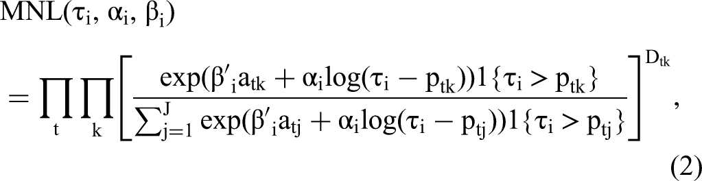
We adopt the convenient logarithmic specification of indirect utility, similar to that of Berry, Levinsohn, and Pakes (1995), because it results in simulated demand curves that are continuous in price, a necessary condition for the simulation-based computation of competitive equilibrium prices. The expression for the choice probability of alternative k in the overall likelihood is then

$$\begin{array}{rl}& \mathrm{MNL}({\tau }_{\mathrm{i}},{\alpha }_{\mathrm{i}},{\beta }_{\mathrm{i}})\\ & =\prod _{\mathrm{t}}\prod _{\mathrm{k}}{\left[{\displaystyle \frac{\exp ({{\beta }^{\mathrm{\prime }}}_{\mathrm{i}}{\mathrm{a}}_{\mathrm{tk}}+{\alpha }_{\mathrm{i}}\log ({\tau }_{\mathrm{i}}-{\mathrm{p}}_{\mathrm{tk}}))1\{{\tau }_{\mathrm{i}}>{\mathrm{p}}_{\mathrm{tk}}\}}{{\sum }_{\mathrm{j}=1}^{\mathrm{J}}\exp ({{\beta }^{\mathrm{\prime }}}_{\mathrm{i}}{\mathrm{a}}_{\mathrm{tj}}+{\alpha }_{\mathrm{i}}\log ({\tau }_{\mathrm{i}}-{\mathrm{p}}_{\mathrm{tj}}))1\{{\tau }_{\mathrm{i}}>{\mathrm{p}}_{\mathrm{tj}}\}}}\right]}^{{\mathrm{D}}_{\mathrm{tk}}},\end{array}$$

(2)

where D_tk = 1 if alternative k is selected in choice task t and 0 otherwise, a_tk characterizes the nonprice attribute levels of alternative k in task t, and p_tk is the corresponding price.

Random Coefficient Model

We adopt the marginal-conditional decomposition in Pachali, Kurz, and Otter (2020) to sign-constrain the budget and price coefficients in line with economic theory in the flexible S-component mixture of normals hierarchical prior/random coefficient distribution:

$$\left(\begin{array}{c}{\tau }_{\mathrm{i}}^{*}\\ {\alpha }_{\mathrm{i}}^{*}\\ {\beta }_{\mathrm{i}}^{*}\end{array}\right)=\left(\begin{array}{c}\log ({\tau }_{\mathrm{i}})\\ \log ({\alpha }_{\mathrm{i}})\\ {\beta }_{\mathrm{i}}\end{array}\right)\sim \sum _{\mathrm{s}=1}^{\mathrm{S}}{\eta }_{\mathrm{s}}\mathrm{N}({\mu }_{\mathrm{s}}^{*}+({\mathrm{\Delta }}^{*}{)}^{\mathrm{\prime }}{\overline{\mathrm{Z}}}_{\mathrm{i}},{\mathrm{V}}_{\mathrm{s}}^{*}),$$

(3)

where ${\overline{\mathrm{Z}}}_{\mathrm{i}}$ is row i of the demeaned matrix of financial demographic variables, such as disposable income and liquid funds; Δ* relates demographics to budget, price, and remaining demand coefficients (as suggested by, e.g., Petrin [2002]); $({\mu }_{\mathrm{s}}^{*},{\mathrm{V}}_{\mathrm{s}}^{*})$ are component-specific mean and variance-covariance parameters; and η_s measures the weight of mixture component s. We need to take into account that Δ* is estimated on the log scale, and Web Appendix B shows how to arrive at the estimates of the relationship between demographics and sign-constrained demand parameters. We decide the number of mixture components (S) in the empirical application by comparing approximations to the marginal likelihood of different model specifications (similarly to the approach proposed in Dubé, Hitsch, and Rossi [2010]).

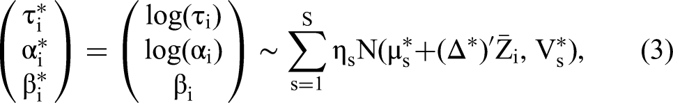
The financial demographic variables provide useful information about differences in budgets across respondents and thus increase the accuracy as well as the efficiency of the random coefficient model. According to household finance theory (e.g., Deaton 1991), the monthly income remaining after accounting for fixed expenditures and the value of liquid assets readily available for spending are important determinants of the budget a consumer can spend on a high-ticket item such as a new laptop. It is thus useful to add this component of observed heterogeneity as data-based information about unobserved budget constraints. Moreover, the posterior relationship between financial demographic variables and model parameters can help with the substantive interpretation of parameters in the individual-level likelihood. For example, finding that financial demographics explain budget variation further substantiates the interpretation of the budget parameter in the model.

Markov Chain Monte Carlo Estimation

Figure 1 shows the directed acyclic graph (DAG) corresponding to the model described in Equation 1 and Equation 3, where ind $\in \{1,\dots ,\mathrm{S}\}$ denotes the mixture component membership of a respondent. The DAG illustrates that both respondents’ financial variables and their stated budgets (before conducting the choice tasks in the experiment) relate to unobserved, true budgets τ_i. These two additional data ingredients provide information about unobserved budgets over and above what can be inferred from the choice model only, facilitating empirical identification beyond subjective functional form assumptions.

Figure 1.

Inferring Budgets from Choice Data, Stated Budgets and Financial Demographics DAG.

Algorithm 1 summarizes each step of our Markov chain Monte Carlo (MCMC) method, based on the DAG in Figure 1. The priors and subjective priors for the upper-level coefficients are specified as proposed in Pachali, Kurz, and Otter (2020), accounting for the change of variable to impose economic constraints. The prior for the error variance follows an inverse chi-square distribution with subjective prior parameters specified as suggested in Rossi, Allenby, and McCulloch (2005).

Algorithm 1.

Markov Chain Monte Carlo Stated Budgets.

For i = 1, …, N, update latent budget, price sensitivity, and remaining utility coefficients (τi, αi, βi) in a Metropolis step (Rossi, Allenby, and McCulloch 2005), with the likelihood function as specified in Equation 1, and conditional on the respondent's stated budget and the current state of the error variance ( ${\mathrm{b}}_{\mathrm{i}},{\sigma }_{\mathrm{error}}^2$ ): $${\tau }_{\mathrm{i}},{\alpha }_{\mathrm{i}},{\beta }_{\mathrm{i}}|{\mu }_{\mathrm{in}{\mathrm{d}}_{\mathrm{i}}}^{*},{\mathrm{V}}_{\mathrm{in}{\mathrm{d}}_{\mathrm{i}}}^{*},\mathrm{in}{\mathrm{d}}_{\mathrm{i}},{\mathrm{\Delta }}^{*},{\mathrm{y}}_{\mathrm{i}},{\mathrm{b}}_{\mathrm{i}},{\sigma }_{\mathrm{error}}^2,{\overline{\mathrm{Z}}}_{\mathrm{i}}.$$ Update upper-level model parameters on the basis of the marginal-conditional decomposition as described in Pachali, Kurz, and Otter (2020), using the updated individual-level coefficients as “data”: $$\{{\mu }_{\mathrm{s}}^{*},{\mathrm{V}}_{\mathrm{s}}^{*},{\eta }_{\mathrm{s}}\}|\{{\tau }_{\mathrm{i}},{\alpha }_{\mathrm{i}},{\beta }_{\mathrm{i}},\mathrm{in}{\mathrm{d}}_{\mathrm{i}}\}.$$ Perform the conjugate update of ${\sigma }_{\mathrm{error}}^2$ , computing the sum of squared residuals between τi and bi as another step of the sampler: $${\sigma }_{\mathrm{error}}^2|{\tau }_{\mathrm{i}},{\mathrm{b}}_{\mathrm{i}}.$$

We note that it is also possible to infer respondents’ budgets {τ_i} purely from the observed choice data {y_i} and respondents’ financial demographics $\{{\overline{\mathrm{Z}}}_{\mathrm{i}}\}$ without accounting for the stated budgets {b_i}. The MCMC method in Algorithm 1 then simplifies to Step 1 and Step 2, omitting ${\mathrm{b}}_{\mathrm{i}},{\sigma }_{\mathrm{error}}^2$ . The contrast of the two models—with and without accounting for stated budgets—illustrates the benefits of adding stated budgets to the model as in Figure 1. In theory, latent budgets are identifiable from variations in choice data alone. In a nutshell, empirical identification of budgets comes from the violation of the Slutsky symmetry implied by the standard quasi-linear utility model (Abaluck and Adams-Prassl 2021). We provide a detailed argument for identifying latent budgets from variations in data in Web Appendix C.

Benchmark Models

Next, we describe the benchmark models that we include in the empirical analyses. A widely adopted choice model assumes quasi-linear demand, omitting the individual-specific index i for simplicity:

$$\mathrm{P}{\mathrm{r}}_{\mathrm{k}}(\beta ,{\beta }_{\mathrm{p}})={\displaystyle \frac{\exp ({\beta }^{\mathrm{\prime }}{\mathrm{a}}_{\mathrm{k}}-{\beta }_{\mathrm{p}}{\mathrm{p}}_{\mathrm{k}})}{{\sum }_{\mathrm{j}=1}^{\mathrm{J}}\exp ({\beta }^{\mathrm{\prime }}{\mathrm{a}}_{\mathrm{j}}-{\beta }_{\mathrm{p}}{\mathrm{p}}_{\mathrm{j}})}.}$$

(4)

It is straightforward to show that the model in Equation 4 is equivalent to the choice model in Equation 2 if the specified budget is much larger than the category-specific price level. The model thus assumes that all prices in a choice set are within the feasible set of alternatives. The price coefficient β_p (coupled with corresponding adjustments of β) approximates that respondents may consistently reject high prices because of budget constraints. From its prevalence in empirical applications, Equation 4 could be regarded as the de facto standard in the marketing literature.

Allenby et al. (2014a) rely on this model but suggest removing respondents on the basis of small marginal likelihoods from the estimation sample to improve inferred prices from CBC optimization exercises. As some may see dropping information-poor respondents as an alternative to accounting for unobserved budgets, we include the Allenby et al. (2014a) model as a benchmark model in the empirical application.

Another popular model for nonlinear price effects is estimating K − 1 price dummies for the K different prices characterizing the choice environment under study. At the level of observed demand, the concept of a budget translates into a highly nonlinear reaction to price, and we therefore consider the dummy-coded model as another benchmark specification.

Characterizing the Bias from Ignoring the Budget Constraint

We next show in a simulation study that benchmark models insufficiently approximate consumers’ latent budget constraints. The first part presents the consequences for model fit, and the second part illustrates the implications for aggregate demand, equilibrium prices, and realized brand profits.

Suppose consumers have heterogeneous preferences for two differentiated brands, A and B. On average, consumers prefer Brand A over Brand B, and ${\overline{\beta }}_{\mathrm{A}}=6>{\overline{\beta }}_{\mathrm{B}}=3$ . Further, assume that about 80% of consumers in the population are budget-constrained and cannot afford the largest price of 4.5 shown in the design. ¹⁰

Each of N = 1,000 simulated consumers makes T = 4 choices from choice sets featuring both inside brands and the outside good. ¹¹ Similarly to our empirical application, we rely on a sensible price grid covering nine possible prices. Prices are uniformly drawn from the set {.5, 1, 1.5, 2, 2.5, 3, 3.5, 4, 4.5}. We use these data to fit the data-generating budget model with the individual-level likelihood defined in Equation 2, the “standard model” with individual-level likelihood given by Equation 4, and the dummy price model accounting for any nonlinear price responses. ¹²

Here, we aim to show that ignoring unobserved budgets in benchmark models biases inferences about aggregate demand. The simulation study does not incorporate the financial demographics or stated budgets that we collect as additional data in our empirical application. ¹³

Evaluation of Model Fit

For the fit comparison, we rely on the marginal aggregate price–demand relationship in the simulated data. We evaluate the fit of the models in terms of their ability to match the model-free and data-based empirical demand curve as shown in Figure 2.

Figure 2.

Comparing Data-Based and Model-Based Aggregate Demand Curves.

In comparison with the benchmarks, we see that the marginal aggregate predictions from the model that infers budgets are close to the data-based curve at every price included in the design. By contrast, it is visually apparent that the dummy-coded model does not perform significantly better than the standard quasi-linear model (Equation 4) and shows the worst fit at many price points. ¹⁴ Notably, the implied aggregate demand curve of the dummy-coded model becomes essentially flat at larger prices and, consequently, overestimates market share at the highest price of 4.5. Table 1 shows all benchmark models’ root mean square error (RMSE) relative to the true data-generating aggregate demand curve computed at the different price points. ¹⁵ The numbers confirm that the dummy model does not improve fit relative to the standard model. This finding is because the approximation of budget constraints through dummy-coded price effects can be poor in finite data sets, especially in hierarchical settings with heterogeneous budget constraints.

Table 1.

RMSE Relative to the Data-Based Aggregate Demand Curve.

Model	RMSE
Standard model	1.51 (.020)
Inferred budgets	1.36 (.019)
Dummy coded	2.42 (.021)

Notes: “Inferred budgets” is estimated on the basis of Step 1 and Step 2 in Algorithm 1, omitting ${\mathrm{b}}_{\mathrm{i}},{\sigma }_{\mathrm{error}}^2$ . Standard errors are in parentheses.

Implications for Aggregate Demand, Equilibrium Prices, and Brand Profits

Next, we investigate differences in market-level predictions between the models. Equation 5 defines the posterior predictive market share of choice alternative k given prices p and choice set configuration A under the model that incorporates budgets. ¹⁶ Posterior predictive market shares in Equation 5 are just fixed numbers given the posterior distributions to be integrated over. We compute corresponding quantities for benchmark models analogously.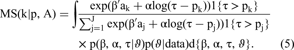

$$\begin{array}{rl}\mathrm{MS}(\mathrm{k}|\mathrm{p},\mathrm{A})=\int & {\displaystyle \frac{\exp ({\beta }^{\mathrm{\prime }}{\mathrm{a}}_{\mathrm{k}}+\alpha \log (\tau -{\mathrm{p}}_{\mathrm{k}}))1\{\tau >{\mathrm{p}}_{\mathrm{k}}\}}{{\sum }_{\mathrm{j}=1}^{\mathrm{J}}\exp ({\beta }^{\mathrm{\prime }}{\mathrm{a}}_{\mathrm{j}}+\alpha \log (\tau -{\mathrm{p}}_{\mathrm{j}}))1\{\tau >{\mathrm{p}}_{\mathrm{j}}\}}}\\ & \times \mathrm{p}(\beta ,\alpha ,\tau |\vartheta )\mathrm{p}(\vartheta |\mathrm{data})\mathrm{d}\{\beta ,\alpha ,\tau ,\vartheta \}.\end{array}$$

(5)

As an illustration, we compute posterior predictive shares in a choice set that offers both inside brands at the highest price used in the design (p = 4.5). As a consequence of ignoring consumers’ budget restrictions, the standard model overstates the share of Brand A in this set and understates the share of outside choices (see Table 2). The more flexible dummy-model approximation fails to correct for the bias of the standard model and overstates the market share of Brand A as well, and even more so. Standard models thus predict that too few consumers will stop choosing inside brands if prices become high.

Table 2.

Posterior Predictive Market Shares.

Brand	True	Standard Model	Inferred Budgets	Dummy Coded
Brand A	3.48	5.05	4.29	8.25
Brand B	.29	.55	.51	.54
Outside	96.23	94.40	95.20	91.20

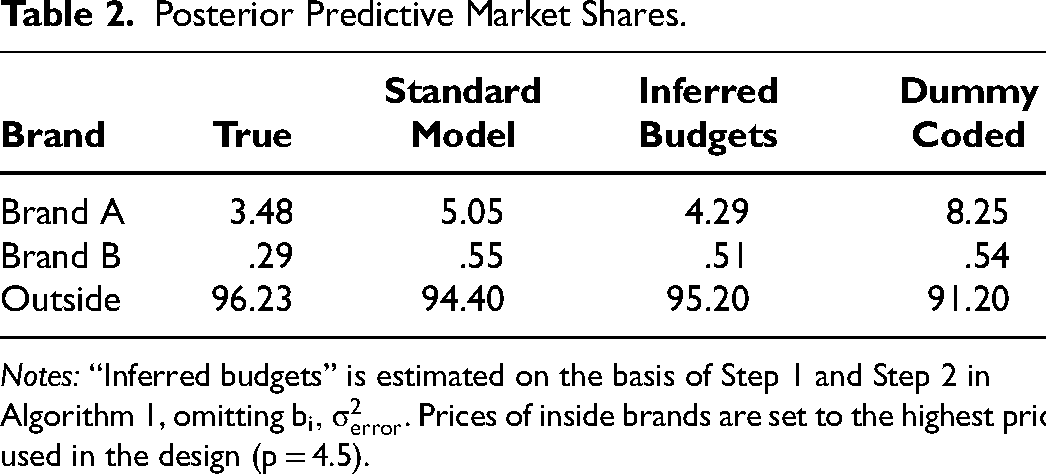
Notes: “Inferred budgets” is estimated on the basis of Step 1 and Step 2 in Algorithm 1, omitting ${\mathrm{b}}_{\mathrm{i}},{\sigma }_{\mathrm{error}}^2$ . Prices of inside brands are set to the highest price used in the design (p = 4.5).

The reason for this failure goes beyond a particular type of shrinkage model employed. The dummy model associates each price level with its own parameter. In expectation, price levels associated with negative parameters translate into low choice probabilities. At the lower end of the sigmoid function that links expected utility to choice probabilities, first derivatives are small, and both first and second derivatives increase (decrease) as utility increases (decreases). Thus, a high price level associated with low choice probabilities will be harder to distinguish from an even higher price level in finite data without a functional form connecting them. Moreover, in a situation where some respondents still find the higher price level acceptable and choose offers at this higher price level, these respondents contribute more information to the inferred population distribution than those that do not, because of the asymmetry of the individual multinomial logit likelihood at the lower end of the sigmoid curve. Note that this applies regardless of the type of shrinkage model or hierarchical prior specification employed.

We next show the implications for equilibrium pricing, a counterfactual outcome that has received recent interest in conjoint studies (e.g., Allenby et al. 2014a; Choi and DeSarbo 1994; Srinivasan, Lovejoy, and Beach 1997). The static Nash equilibrium is defined as a set of prices that simultaneously satisfy all brands’ profit-maximization conditions. We define the kth brand's profit as a function of price, given all other prices as

$$\pi ({\mathrm{p}}_{\mathrm{k}}|{\mathrm{p}}_{-\mathrm{k}})\propto \mathrm{MS}(\mathrm{k}|\mathrm{p},\mathrm{A})({\mathrm{p}}_{\mathrm{k}}-{\mathrm{c}}_{\mathrm{k}}),$$

(6)

where c_k denotes brand-specific, constant marginal costs and A represents the design of product alternatives competing in the market. The proportionality results from ignoring the market size and fixed costs. The pure strategy Nash equilibrium price vector, p*, then solves the first-order conditions (“best-response functions”) of all K brands in the market simultaneously (see Equation 7 for Brand k's condition).

$${\displaystyle \frac{\mathrm{\partial }\pi }{\mathrm{\partial }{\mathrm{p}}_{\mathrm{k}}}\propto {\displaystyle \frac{\mathrm{\partial }}{\mathrm{\partial }{\mathrm{p}}_{\mathrm{k}}}\mathrm{MS}(\mathrm{k}|\mathrm{p},\mathrm{A})({\mathrm{p}}_{\mathrm{k}}-{\mathrm{c}}_{\mathrm{k}})+\mathrm{MS}(\mathrm{k}|\mathrm{p},\mathrm{A}).}}$$

(7)

To compute the equilibrium, we rely on an iterative method (e.g., Allenby et al. 2014a) that computes the optimal price for each brand given other prices until $||{\mathrm{p}}^{\mathrm{r}}-{\mathrm{p}}^{\mathrm{r}-1}||<\mathrm{tol}$ . ¹⁷

A firm's best-response function depends on the derivative of aggregate market share and aggregate market share itself. A necessary condition for the existence of a pure-strategy Nash equilibrium is the continuity of best-response functions, that is, the continuity of market share as a function of price (Caplin and Nalebuff 1991; Friedman 1990). This requirement is obviously fulfilled for the standard linear price model. In the budget model, the logarithmic utility function implies that choice probabilities smoothly approach zero as the price approaches the budget constraint. Thus, simulated changes in aggregate demand result from mixing over continuous changes in heterogeneous choice probabilities and, therefore, are continuous regardless of the number of simulation draws. However, this minimum requirement is not satisfied for the dummy-coded model as the indirect utility function implied by the K – 1 dummy price coefficients is noncontinuous. To preserve continuity, we fit smoothing splines (Hastie and Tibshirani 1986) to every draw from the posterior distribution of the price dummies. We then compute equilibrium prices integrating over the thus processed posterior draws.

Table 3 shows inferred equilibrium prices implied by the different models. As expected, the model inferring unobserved budgets predicts prices close to the truth. However, note that equilibrium prices conditional on posterior uncertainty (finite N) are different from the truth by definition of the objective function that involves expectations of nonlinear functions with respect to the posterior. In comparison, the standard model clearly overstates the equilibrium prices of both brands. The reason is that the model fails to recognize the loss in market share from violating consumers’ budget constraints. It is noteworthy that the dummy-coded model implies a further increased price for Brand A. This is a direct consequence of overestimating demand and the slope of the demand curve at high prices by this model, a result that we replicate in our empirical application. ¹⁸

Table 3.

Equilibrium Prices.

Brand	Max. Price	True	Standard Model	Inferred Budgets	Dummy Coded
Brand A	4.50	2.99	3.18	3.05	4.50
Brand B	4.50	2.49	2.65	2.56	2.45
Outside	.00	.00	.00	.00	.00

Notes: “Inferred budgets” is estimated on the basis of Step 1 and Step 2 in Algorithm 1, omitting ${\mathrm{b}}_{\mathrm{i}},{\sigma }_{\mathrm{error}}^2$ . Marginal costs were set to 2 for both brands in this illustration.

The resulting losses in brand profits from the suboptimal actions suggested by the models are displayed in Table 4. For this purpose, we evaluate the losses of profits for Brand k implied by prices of model m, ${\mathrm{p}}_{\mathrm{k}}^{\mathrm{m}}$ , ${\mathrm{L}}_{\mathrm{k}}=[\pi ({\mathrm{p}}_{\mathrm{k}}^{\mathrm{true}}|{\mathrm{p}}_{-\mathrm{k}}^{\mathrm{true}})-\pi ({\mathrm{p}}_{\mathrm{k}}^{\mathrm{m}}|{\mathrm{p}}_{-\mathrm{k}}^{\mathrm{true}})]/\pi ({\mathrm{p}}_{\mathrm{k}}^{\mathrm{m}}|{\mathrm{p}}_{-\mathrm{k}}^{\mathrm{true}})\times 100$ , where profits $\pi (\cdot )$ are computed using the data-generating true preference distribution.

Table 4.

Average Loss in Brand Profits.

Model	Profit Loss (%)
Standard model	3.31
Inferred budgets	.57
Dummy coded	37.96

Notes: “Inferred budgets” is estimated on the basis of Step 1 and Step 2 in Algorithm 1, omitting ${\mathrm{b}}_{\mathrm{i}},{\sigma }_{\mathrm{error}}^2$ . Losses are computed relative to optimal prices implied by the true preference distribution in the data-generating process. Marginal costs were set to 2 for both brands in this illustration.

We also investigate differences in optimal prices and losses in brand profits for a cost grid considering 30 scenarios in the range of .1 to 3. Figure 3 shows that the benchmark models overestimate the prices of both brands in various cost scenarios, leading to substantial profit losses (Figure 4).

Figure 3.

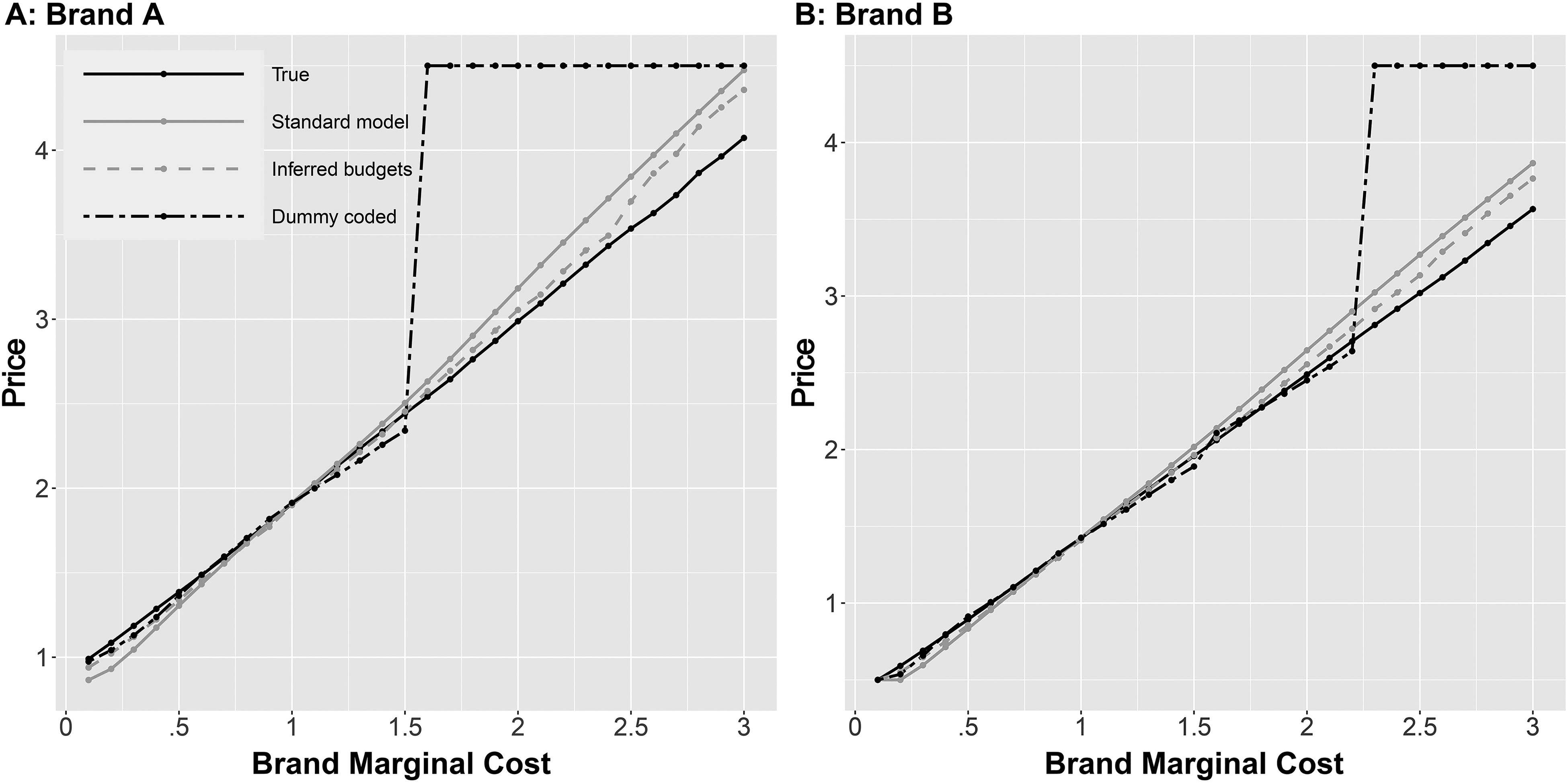
Equilibrium Prices Under Different Cost Scenarios.

Figure 4.

Average Loss in Brand Profits Under Different Cost Scenarios.

Finally, we illustrate the implications for profit losses as a function of the fraction of budget-constrained consumers in the data-generating process. We find that differences in profit losses start to vanish between the standard linear price model and the proposed model if less than 20% of consumers are budget-constrained in the population (see Table W1 in Web Appendix D). By contrast, the dummy-coded model still implies severe profit losses even if only 10% of consumers are budget-constrained in the data-generating process (see Table W1 in Web Appendix D).

Discrete-Choice Experiment on Preferences for Laptops

So far, we have derived a discrete-choice model that infers latent budgets by leveraging additional data about respondents’ financial demographics and stated budgets (see Algorithm 1). This section illustrates the empirical performance of the proposed budget model and compares its fit to several benchmark specifications in the literature. We proceed by discussing the consequences of either ignoring or insufficiently approximating consumers’ budgets for inferred price–demand curves and competitive pricing using a discrete-choice experiment investigating preferences for high-end laptops. A unique feature of our data set is that it contains several metrics characterizing respondents’ financial situation (e.g., disposable income) that should enter the determination of budgets according to economic theory and includes budgets that the respondents stated before evaluating the 15 choice tasks.

Design

Our empirical application uses data from a discrete-choice experiment investigating preferences for higher-end premium laptops. A total of 1,000 respondents, carefully prescreened for market membership, participated in the experiment. Every respondent completed 15 choice sets, comprising three inside options and the outside good. The experiment featured eight attributes, including a seven-level brand attribute; Table 5 summarizes the attributes and corresponding levels.

Table 5.

Description of Attributes of Laptop Data.

Attributes	Levels
Price in EUR	600, 1,000, 1,400, 1,800, 2,200, 2,600, 3,000, 3,500, 4,000
Brand	Dell, Lenovo, Hewlett-Packard (HP), MaxData, Acer, Apple, Asus
Memory	8 GB, 16 GB, 32 GB, 64 GB
Screen size (in inches)	12, 13, 14, 15, 17
Resolution	1,280 × 1,024, 1,600 × 1,200, 1,920 × 1,080, 1,920 × 1,200, 3,840 × 2,160
Processor	AMD Athlon, AMD Ryzen 3, AMD Ryzen 5, Intel Core i3, Intel Core i5, Intel Core i7, Apple M1
Hard disk	HDD (.3 GB/sec), SSD (.6 GB/sec), SSD (1 GB/sec), SSD (2.5 GB/sec), SSD (3.1 GB/sec)
Size of hard disk	250 GB, 512 GB, 1 TB, 2 TB

We collected information about respondents’ demographics. A distinguishing feature of our data set is that it covers a rich set of household finance characteristics, such as the household monthly gross income, monthly disposable income after typical monthly expenditures, the respondent's planned payment method, ownership of houses (real estate), and value of liquid funds available for spending (Table 6). We include some of these financial variables (i.e., disposable income, liquid funds) in the hierarchical prior as causal parents of latent budgets (see the DAG in Figure 1), as suggested by household finance theory (e.g., Deaton 1991). We also directly asked respondents to state “the maximum amount you will be able to spend on your next laptop purchase” (i.e., the “stated budget”) after they were briefed about the covered attribute levels, but before they evaluated the 15 choice tasks in the experiment. We informed respondents carefully about the included attribute levels in the study before asking about their budget to minimize the impact of a potential bias, such as learning about product configurations while answering the choice tasks.

Table 6.

Respondents' Financial Variables in the Laptop Study.

Demographics	Levels
Monthly gross income (in EUR)	Continuous
Monthly net income after typical expenditures (in EUR)	Continuous
Stated budget for next laptop purchase (in EUR)	Continuous
Planned payment method	Cash, paying by installments
Ownership of real estate	Yes, no
Liquid funds (in EUR)	Six predefined intervalsa

^a

Smaller than 5,000; [5,000, 9,999]; [10,000, 19,999]; [20,000, 49,999]; [50,000, 100,000]; larger than 100,000.

The stated budget suffers from measurement error (e.g., Moore, Stinson, and Welniak 2000) and is thus only an indication of the respondent's true latent budget. As a consequence, 54.43% of respondents slightly exceeded the initially stated budget by choosing larger prices in the experiment. Most of the differences between the initially stated budget and the maximum price chosen are small among respondents. The mean equals 159.5 EUR (median 100 EUR), and the stated budget is on average 10.4% (median 8.3%) smaller than the maximum price chosen in the experiment. ¹⁹ These stated budgets, potentially afflicted with measurement error, are fallible indicators and thus add information to the individual-level likelihood functions (see the DAG in Figure 1).

In an additional analysis, we rely on stated budgets to validate the accuracy of our budget estimates in the demand model that excludes the likelihood information in stated budgets. The MCMC method in Algorithm 1 then simplifies to Step 1 and Step 2, omitting ${\mathrm{b}}_{\mathrm{i}},{\sigma }_{\mathrm{error}}^2$ . In this validation exercise, respondents’ latent budgets {τ_i} are thus purely inferred from choice data and respondents’ financial demographics without accounting for stated budgets in the estimation.

Data Quality Assurances

The data provider ensures the quality of collected data through various steps. All respondents originated from permission-based panels. Participating panelists are validated on the basis of their IP addresses and their behavior in other surveys they opted into. This involves cross-checking responses to screening and demographic questions across different surveys each panelist had participated in. In addition, we remove panelists from the sample if they responded in an unreliable manner by (1) exceeding the stated budget in the experiment by 50% or more, (2) not reporting monthly income, and (3) only choosing the outside good throughout the experimental tasks. These steps reduce the initial sample of 1,000 respondents to 643 considered respondents in our analysis. Consistent with the evidence from our practitioner survey mentioned previously, the possibility of incentive-aligned experiments was dismissed on the basis of cost and implementation considerations, as well as the understanding that, because of income effects, endowing respondents with significant budgets may invalidate inference for the target market of consumers not endowed this way. ²⁰

Model-Free Descriptives

We report several model-free summaries of the data to illustrate how respondents react to price changes in the choice experiment and how respondents’ financial situations affect the reported amount of money available for spending on the next laptop (“stated budget”).

Maximum price chosen and empirical aggregate demand

Figure 5 summarizes the empirical distribution of the maximum prices chosen by each respondent considered in the analysis, where the maximum is over repeated measurements for each respondent. The figure shows that only 23 respondents (i.e., 3.58% of 643 respondents) chose a laptop offered at the maximum price of 4,000 EUR in the choice experiment. ²¹ The inclusion of these large prices facilitates the identification of the distribution of budgets in our data.

Figure 5.

Empirical Frequency Distribution of the Maximum Price Chosen.

Figure 6 shows the data-based marginal demand curve computed directly from our choice data. Specifically, we compute the choice share (“demand”) at every unique price in the experiment as the number of times a laptop was chosen at a certain price, for example 2,200 EUR, divided by the number of times a laptop was shown in a choice set at this price. This procedure is also known as count analysis in the CBC literature, as it consists of counting the fraction of wins of an attribute level in the experiment. The result is the empirical aggregate marginal reaction to price. However, note that the curve in Figure 6 does not isolate the impact of price as our design induces higher prices for laptops with better attribute levels in expectation. Nevertheless, Figure 6 shows that respondents react strongly to price in the experiment. For example, the choice shares substantially drop to about 5% at a price of 2,200 EUR. For even larger prices, demand becomes less elastic as many price-sensitive respondents have already chosen the outside good because of their budget restrictions, as we will show. At the price of 4,000 EUR, the choice share is almost zero and equal to 1.7%. We will subsequently revisit this summary of our data to assess the differences between model-based predictions.

Figure 6.

Data-Based Aggregate Demand Curve.

Distribution of stated budgets

Figure 7 shows the empirical distribution of respondents’ stated budgets for the planned purchase of a laptop. The distribution of stated budgets is fairly skewed across the consumer population, with the mean budget equal to 1,157 EUR (median 1,000 EUR). Furthermore, some respondents stated they that had a large amount of money to spend on a new laptop (beyond 2,000 EUR) in the distribution's right tail.

Figure 7.

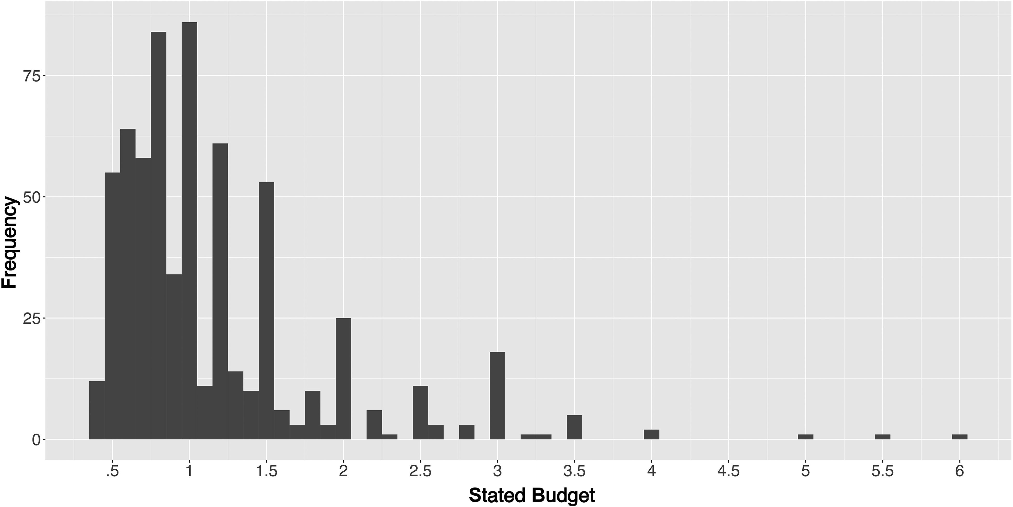
Distribution of Respondents’ Stated Budgets.

Household finance theory suggests that disposable income and the availability of liquid funds causally influence the amount of money available to spend on a laptop (e.g., Deaton 1991). Conditioning on disposable income and liquid funds, causal parents such as gross income ²² or illiquid assets (e.g., property ownership) should thus not matter for the budget constraint. Table W2 in Web Appendix E empirically corroborates this reasoning in our setting. By regressing respondents’ stated budgets on the financial variables mentioned, we find significantly positive conditional direct effects from disposable income and liquid funds and null effects for gross income and property ownership (see Table W2 in Web Appendix E).

Inferred Budget Distribution

We next discuss the inferred budget distribution implied by the proposed model accounting for respondents’ stated budgets in the estimation (see Algorithm 1). ²³ Figure 8 shows the posterior budget distribution characterizing the population of consumers implied by the one-component normal mixture model. Web Appendix F shows that adding more mixture components does not change our inference. We estimate that approximately 96.4% of consumers in the population have budgets for laptops smaller than the highest price (4,000 EUR) shown in the design and are effectively budget-constrained. Web Appendix G illustrates the benefits of accounting for stated budgets in the estimation, compared with the model that infers latent budgets purely from choice data. Figure W3 in Web Appendix G visually depicts that accounting for stated budgets implies thinner tails and less extreme predicted budgets in the posterior distribution. Even though the inclusion of stated budgets improves inference regarding the tails of the distribution, Web Appendix H demonstrates convergent validity between stated budgets and budgets only inferred from the choice part of the likelihood in Equation 2. We find that inferred posterior mean budgets strongly and positively correlate with respondents’ stated budgets when stated budgets are not included in the model as likelihood information (see Table W5 in Web Appendix H).

Figure 8.

Posterior Predictive Density of Budgets.

Our model also infers the empirical relation of respondents’ budgets with financial consumer demographics. Table 7 reports estimated relations between the relevant consumer financial demographics, the budget, and the price coefficient α in the utility function (Equation 2) in Columns 1 and 2. ²⁴ Column 3 in Table 7 reports estimated relations between consumer demographics and the price coefficient β_p in the standard quasi-linear model (Equation 4) for comparison. ²⁵

Table 7.

Estimated Relationship Between Demand Model Coefficients and Financial Demographics.

	W. Stated Budgets		Standard Model
	Budget Coeff.	Price Coeff.: Alpha	Price Coeff.
Disposable income	.051***	−.002	.552**
Liquid funds	.005***	−.001	.085***
Paying by installments	.292**	−.325	2.305

*p < .1. **p < .05. ***p < .01.

Notes: The first two columns show the estimated relationship for the model with stated budgets (see Algorithm 1). The last column shows the estimated relation for the standard linear price model.

The results in Table 7 show that the estimates of budgets relate to consumer financial characteristics as predicted by household finance theory. For example, on average, respondents with higher disposable income and liquid funds have larger budgets for purchasing a laptop. Moreover, we find that inferred price coefficients are independent of disposable income and the value of liquid assets a posteriori. These outcomes align with economic and household finance theory, implying that respondents screen out high prices because of budget constraints. By contrast, the standard model implies that respondents with higher disposable income are universally less price sensitive in an attempt to approximate budget restrictions.

Evaluation of Model Fit

Next, we compare the fit of the benchmark specifications illustrating the superior performance of the proposed budget model. For the fit comparison, we leverage the marginal aggregate price–demand relationship in our data, as in the simulation study. For a fair comparison, the empirical curve excludes observations from information-poor respondents as identified by the sample-censoring approach. We evaluate the fit of the models as their ability to match the model-free and data-based empirical demand curve shown in Figure 9.

Figure 9.

Comparing Data-Based and Model-Based Aggregate Demand Curves.

To keep the figure visually accessible, we omit the aggregate demand curve implied by the standard model without censoring. We see that the standard quasi-linear model (Equation 4) computed on the basis of the censored sample overestimates marginal aggregate demand at low prices, underestimates demand at medium prices, and again overestimates demand at the highest prices included in the experiment (prices higher than 3,500 EUR). The dummy-coded model seems to have little improvement over the standard model and vastly overpredicts demand at low prices and understates demand at medium prices. ²⁶ However, at high prices (higher than 3,500 EUR), the dummy-coded model comes closer to the observed curve. In comparison, the marginal aggregate predictions from the model that accounts for budgets are closer to the observed curve at every price included in the design.

Finally, Table 8 shows the RMSE of all benchmark models relative to the empirical (data-based) aggregate demand curve computed at the different price points in this study. We find that accounting for unobserved budgets substantially improves model fit (RMSE is reduced by 65.42% compared with the best-fitting standard model), while dropping respondents on the basis of low marginal likelihoods does not enhance model fit. This suggests that reducing the sample size deteriorates the inference of consumer preferences in the target population. The dummy-coded model does not improve fit relative to the standard model and is far behind the performance of the budget model. Note that the dummy-coded model may appear flexible at first glance but is likely overparameterized as we need to estimate eight different price dummies in this application. The approximation of budget constraints through dummy-coded price effects will thus be poor in the “small T–large N” setting typical of CBC data in marketing and specifically in hierarchical settings with heterogeneous budget constraints. As explained previously, the reason is the shape of the sigmoid function that connects expected utilities to choice probabilities.

Table 8.

RMSE Relative to the Data-Based Aggregate Demand Curve.

Model	RMSE
Standard model	2.40 (.016)
Standard model (censored sample)	2.58 (.016)
W. stated budgets	.83 (.013)
Dummy-coded model	3.05 (.017)

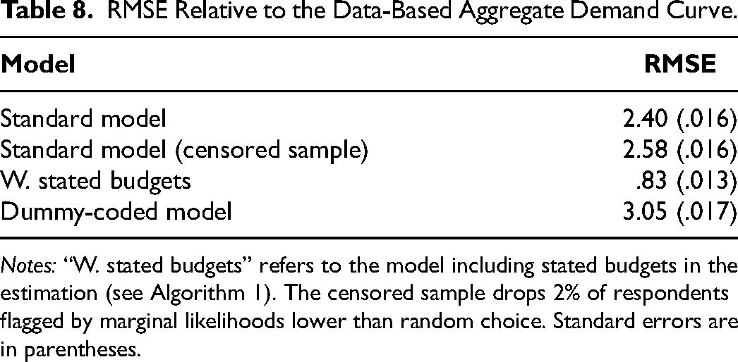
Notes: “W. stated budgets” refers to the model including stated budgets in the estimation (see Algorithm 1). The censored sample drops 2% of respondents flagged by marginal likelihoods lower than random choice. Standard errors are in parentheses.

Implications for Aggregate Demand and Equilibrium Prices

Next, we discuss the consequences for aggregate demand and equilibrium prices. Table 9 summarizes the market scenario we assume, illustrating the consequences of different model specifications for aggregate demand and pricing.

Table 9.

Product Specifications in Market Scenario.

	Memory	Screen Size	Resolution	Processor	Hard Disk	Size of Hard Disk
Dell	32 GB	15 inch	3,840 × 2,160	Intel i7	SSD (3.1 GB/sec)	1 TB
Lenovo	32 GB	15 inch	1,920 × 1,200	AMD Ryzen 5	SSD (2.5 GB/sec)	512 GB
Hewlett-Packard (HP)	64 GB	17 inch	1,920 × 1,200	Intel i7	SSD (3.1 GB/sec)	2 TB
MaxData	8 GB	14 inch	1,280 × 1,024	Intel i3	SSD (1 GB/sec)	250 GB
Acer	8 GB	15 inch	1,280 × 1,024	AMD Ryzen 3	HDD (.3 GB/sec)	250 GB
Apple	64 GB	15 inch	3,840 × 2,160	Apple M1	SSD (3.1 GB/sec)	2 TB
Asus	8 GB	15 inch	1,600 × 1,200	Intel i5	SSD (.6 GB/sec)	250 GB

We first investigate differences in market-level predictions between the benchmark models and the proposed model that includes stated budgets in the estimation (see Algorithm 1). Table 10 summarizes posterior predictive market shares in a scenario where all seven brands as specified in Table 9 are offered at the highest price (4,000 EUR) shown in the design. We find that the standard model overstates the shares of the inside options and understates the share of the outside good. The differences are substantial in size. The standard models that ignore consumers’ budget restrictions predict that too many consumers will be left in the market for laptop computers offered at high prices. For example, the standard linear price model (Equation 4) still predicts that about 10% of consumers in the population would purchase a laptop even if all alternatives were offered for 4,000 EUR. The impact of removing information-poor respondents from the sample to correct this bias is small, according to Table 10. The dummy-coded model provides marginal improvement over the standard linear price model but fails to account for latent budgets adequately. The problem of the dummy-coded model becomes more evident when model-based aggregate demand predictions are considered. Figure 10 plots aggregate posterior demand curves for the premium brand Apple, assuming the respective competitors offer laptops at the highest price.

Figure 10.

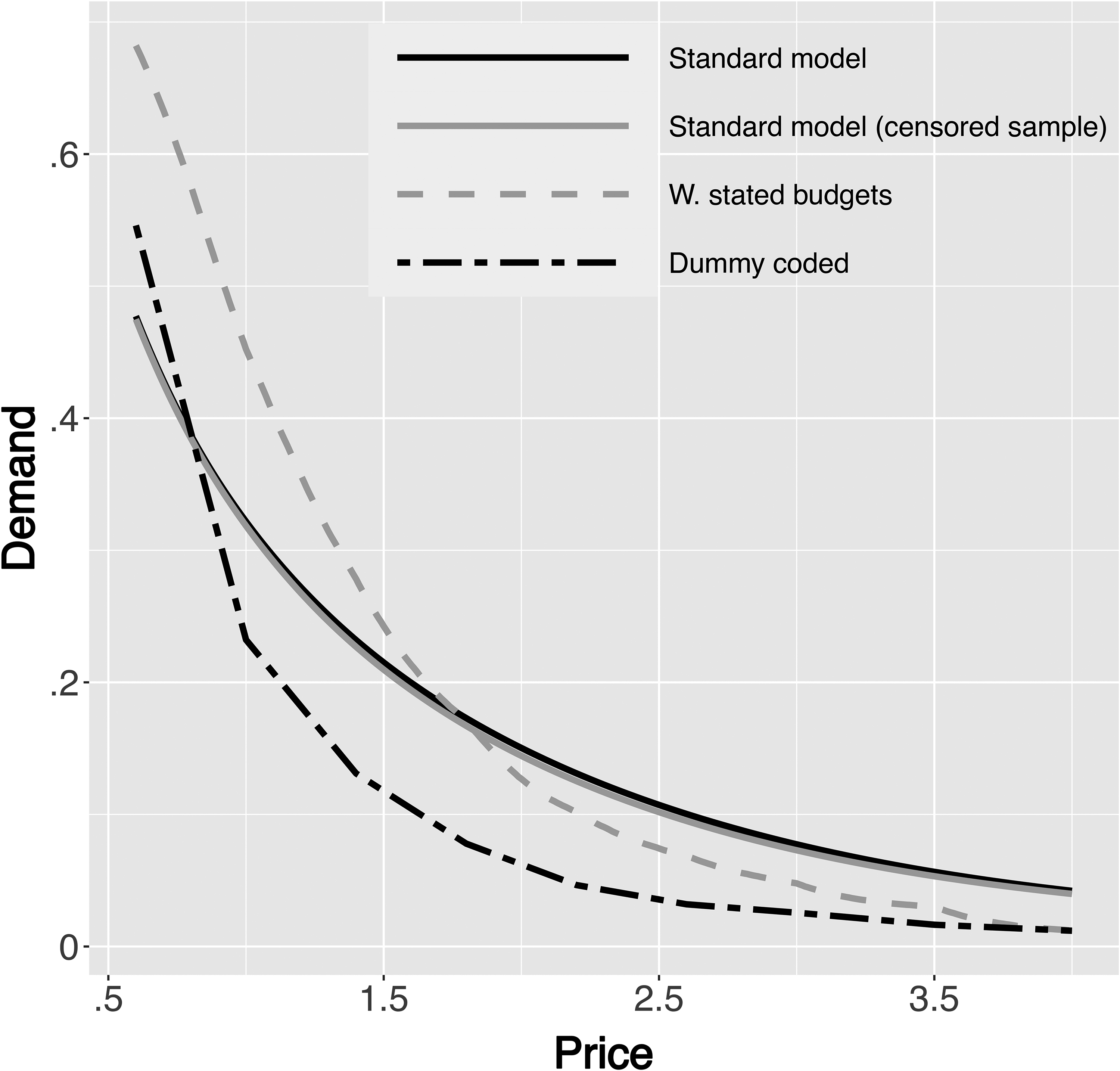
Posterior Predictive Demand Curves for the Apple Laptop.

Table 10.

Posterior Predictive Market Shares.

	Standard Model	Standard Model (Censored Sample)	W. Stated Budgets	Dummy Coded
Dell	1.54	1.47	.63	1.20
Lenovo	1.07	.87	.46	2.41
Hewlett-Packard (HP)	3.89	3.13	.98	.59
MaxData	.05	.04	.04	1.09
Acer	.11	.08	.07	1.05
Apple	4.21	3.98	1.20	1.19
Asus	.11	.11	.11	1.27
Outside	89.01	90.32	96.51	91.20

Notes: Prices of inside brands are set to the highest price (4,000 EUR) shown in the design. “W. stated budgets” refers to the model including stated budgets in the estimation (see Algorithm 1). The censored sample drops 2% of respondents flagged by marginal likelihoods lower than random choice.

Figure 10 shows that none of the benchmark models can match the predicted demand curve of the model accounting for respondents’ budget constraints. Moreover, it is visually apparent that the demand curve implied by the dummy-coded model becomes flat for prices larger than 2,500 EUR.

Due to the distortions in demand curves, the equilibrium predictions from the standard model also appear misleading. The standard linear price models (with and without censoring the sample) overstate equilibrium prices for the high-end laptops and understate prices for remaining products relative to the model that accounts for the influence of budgets (see Table 11). For example, prices of Dell and Apple laptops are estimated to be about 20.65% and 24.82% more expensive in the linear price model based on the censored sample. The dummy-coded model vastly overstates prices, especially for premium brands, as it implies flat aggregate demand curves attenuating the market share penalty of incremental price increases (Figure 10). In an analysis not reported here, we confirm that qualitative differences between models persist when we lower marginal costs by 25%.

Table 11.

Equilibrium Prices (in EUR).

	Max. Price	Standard Model	Standard Model (Censored Sample)	W. Stated Budgets	Dummy-Coded Model
Dell	4,000.00	2,230.01	2,198.01	1,821.84	2,879.06
Lenovo	4,000.00	2,242.47	2,153.99	1,898.35	3,999.95
Hewlett-Packard (HP)	4,000.00	2,629.69	2,521.87	2,191.30	2,069.65
MaxData	4,000.00	716.18	711.60	759.65	1,198.95
Acer	4,000.00	750.33	743.47	836.11	935.54
Apple	4,000.00	3,236.18	3,243.50	2,598.62	2,966.09
Asus	4,000.00	732.13	723.95	924.68	966.86
Outside	.00	.00	.00	.00	.00

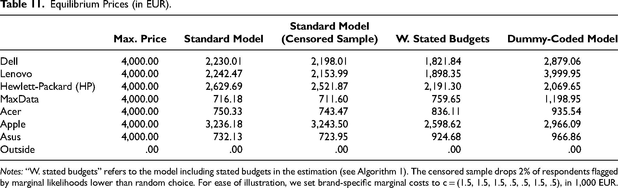
Notes: “W. stated budgets” refers to the model including stated budgets in the estimation (see Algorithm 1). The censored sample drops 2% of respondents flagged by marginal likelihoods lower than random choice. For ease of illustration, we set brand-specific marginal costs to c = (1.5, 1.5, 1.5, .5, .5, 1.5, .5), in 1,000 EUR.

Robustness of Measurement Error Model Specification

We also investigated the performance of an alternative specification of the measurement error model that allows for a common shift (γ) and scale (ψ) bias of stated budgets across respondents; that is, ${\mathrm{b}}_{\mathrm{i}}\sim \mathrm{N}(\gamma +\psi \times {\tau }_{\mathrm{i}},{\sigma }_{\mathrm{error}}^2)$ (see Web Appendix I). This specification picks up systematic differences between the latent and stated budgets. However, as we show in Table W6 in Web Appendix I, the shift and scale measurement error model does not improve fit over the more parsimonious specification in Equation 1. We conjecture that the more flexible model may be influenced unfavorably by individual, more extreme departures between stated budgets and budgets implied by the choice likelihood.

Discussion

Our work makes a theoretically motivated improvement to the standard CBC framework with a new model that estimates respondents’ budget constraints as part of discrete-choice experiments. Despite large stakes being involved in the industry—for example, Apple was awarded about 1 billion USD in damages to be paid by Samsung on the basis of CBC inferences—standard models often ignore budget restrictions, leading to flawed aggregate demand estimates and biased equilibrium price predictions.

As the relevance of budget constraints is strongly supported by economic theory (e.g., Deaton and Muellbauer 1980; Kőszegi and Matějka 2020), we develop a Bayesian model for the inference of latent budget constraints in high-ticket product categories. The proposed method leverages respondents’ stated budgets in the survey, which are potentially afflicted with measurement error, as fallible indicators in the likelihood function and leverages financial demographics as causal parents of budgets in the random coefficient distribution. We show that including these additional data sources helps mitigate the influence of subjective functional form assumptions on the inferred distribution of budgets in the population. This is a desirable property as inference for latent budgets beyond the price support in the experiment would otherwise rely on the extrapolation of a functional form.

We show that omitting the budget constraint substantially biases counterfactual market outcomes in a CBC experiment on high-end laptops. For example, we find that the standard linear price model overstates the equilibrium price for the premium brand Apple by 24.82% even after culling information-poor respondents (Allenby et al. 2014a).

Nonlinear specifications, such as the dummy-coded price model, can approximate consumers’ budget constraints in theory but perform poorly with finite data. An alternative motivation for highly nonlinear price responses is consumer heuristics, such as screening rules for unacceptable attribute levels (e.g., Aribarg et al. 2018; Gilbride and Allenby 2004; Green and Srinivasan 1990). However, an appeal to consumer heuristics translates into a model where consumers could be screening on single attribute, multiple attributes, or even all attributes, which can lead to an overparameterized model and empirical identification problems (see Web Appendix A for a numerical illustration).

We conclude that applied researchers in industry and academia will benefit from estimating budgets in higher-ticket categories. Our methodology is parsimonious, as it only requires estimating one additional parameter at the individual level. Moreover, when the model is fit to data in which budget constraints do not matter given the range of prices investigated, it effectively reverts to the standard quasi-linear model. This is a useful example of a flexible prior structure that allows for the influence of budgets but does not enforce it a priori. In addition, financial background variables and stated budgets collected as part of the CBC survey provide further information about the relevance of budgets.

Going forward, it will be interesting to study budget adjustments as a function of innovative attributes in a product category. Another interesting avenue for future research is the role of the budget constraint in menu-based choice (e.g., Kamakura and Kwak 2012; Kosyakova et al. 2020; Russell and Petersen 2000). Large menus likely preclude the joint choice of large subsets of items because of budgetary limitations. Finally, it would be useful to explore the scope for identification of (distributions of) budgets in aggregate logit models as an alternative to conditioning on a budget distribution such as yearly income based on prior assumptions only (e.g., Berry, Levinsohn, and Pakes 1995).

Supplemental Material

sj-pdf-1-mrj-10.1177_00222437221145283 - Supplemental material for Omitted Budget Constraint Bias and Implications for Competitive Pricing

Supplemental material, sj-pdf-1-mrj-10.1177_00222437221145283 for Omitted Budget Constraint Bias and Implications for Competitive Pricing by Max J. Pachali, Peter Kurz and Thomas Otter in Journal of Marketing Research