Sage Journals: Discover world-class research

Abstract

Using panel data from the Household, Income and Labour Dynamics in Australia survey, this paper analyses the wage gap between the public and private sectors in Australia from 2001 to 2022. The analysis is conducted at both the national and state levels. We found that, since 2014, the public-sector wage premium (nationally) has increased for women but decreased for men, with women's outcomes driving current trends. Additionally, the public-sector wage premium varies significantly across states, indicating that state-level wage-setting forces are more influential than national ones. Our trend analysis reveals that the premium is neither consistently procyclical nor countercyclical. Furthermore, quantile analysis shows that the premium fluctuates across the wage distribution, though not in a uniform pattern over time.

Keywords

Public–private sector wage gap gender regions decompositions quantiles Australia

Introduction

Within the literature there are well-documented differences in the wages of public- and private-sector employees (for recent studies, see Abdallah et al., 2023; Biesenbeek and van der Werff, 2019; Bonaccolto-Töpfer et al., 2022; Choi and Garen, 2021; Makridis, 2021; Murphy et al., 2020). A common finding is that public-sector employees (women in particular) are paid more than their private-sector counterparts and that the gap or premium prevails even in the presence of controls for differences in observable and unobservable characteristics. Studies also reveal significant heterogeneity in the premium across and within countries (Abdallah et al., 2023; Blackaby et al., 2018; Dell’Aringa et al., 2007; Giordano et al., 2015), variation in the premium along the wage distribution (Birch, 2006; Blackaby et al., 1999; Cai and Liu, 2011; Giordano et al., 2015; Mahuteau et al., 2017) and variations in the premium over time (Campos et al., 2017). In some studies the gap is procyclical (Rattsø and Stokke, 2019) and in others it is countercyclical (Abdallah et al., 2023).

Interest in the size and source of the public-sector wage gap arises from considerations of efficiency and equity. In theory, and in the absence of non-competitive forces, the gap should be temporary (e.g., due to skill shortages or labour immobility) and, in the long run, non-existent. However, numerous non-competitive factors influence wage outcomes and drive sectoral differences. Governments, for example, may act as monopolists in certain labour markets such as nursing (Nowak and Preston, 2001) or may use wage policy to deliberately stimulate wage growth for particular groups of workers (e.g., low-paid workers).¹ Governments may also use public-sector wage policy to attract quality public-sector employees and, in turn, affect the quality of services provided (Mahuteau et al., 2017) and/or to control budget deficits. Similarly, fiscal constraints may act as a constraint on public-sector wage offers for some or all groups of workers. Austerity measures adopted in some European countries (post the 2007/08 Global Financial Crisis [GFC]), for example, reduced the public-sector wage gap for high-wage workers (Michael and Christofides, 2020).

Researchers and policy makers are interested in the public–private sector wage gap for several reasons. A public-sector premium may, for example, induce some governments to outsource government work and/or compel the private sector to raise wages to attract labour (Borland et al., 1998). In Australia, institutions such as the Commonwealth Grants Commission closely monitor public–private wage gaps across the states as their remit is to ensure (via fiscal transfers) that states may offer comparable public services given their revenue-generating abilities and associated service delivery costs.

Notwithstanding the significance of public–private wage gaps, the most recent comprehensive assessment of sector wage differentials in Australia is that of Mahuteau et al. (2017). Their analysis employs data from the Household, Income and Labour Dynamics in Australia (HILDA) Survey and covers the period 2001 to 2014. As with many studies they observe a significant public-sector wage premium. At the mean the gap is equal to 5.5% for women and 4.6% for men. They also observe considerable heterogeneity in the premium across states. For example, at the mean, there is an 8.2% premium among men in New South Wales (NSW) and no evidence of a corresponding premium in other states. For women, the public-sector premium varies from 3.1% in Victoria (VIC) to 11.1% for women living in Tasmania (TAS). Mahuteau et al. also show that the premium is larger for low-paid workers and that there is heterogeneity in the low-paid public premium across states.

In this paper data from HILDA are used to revisit the Mahuteau et al. (2017) work and extend the analysis through to 2022. There are reasons to believe that the public–private sector wage differential within and across Australia may have changed since 2001–2014 (the focus of the Mahuteau et al. study). Real wages, for example, have been falling (Treasury, 2023).² Additionally, while wage growth across Australia was faster in the public sector than the private sector over 2001–2022 (Figure 1), a disaggregated analysis shows that in the 2001–2014 period (the period covered by Mahuteau et al.) public-sector wage growth was stronger than private-sector wage growth in all states. In the 2015–2022 period private-sector wage growth was faster than public-sector wage growth in several states, including NSW, South Australia (SA), Western Australia (WA) and TAS (Figures A1 and A2 in Appendix). This likely reflects, in part, government wage policy decisions. In WA, for example, the state Labor government capped public-sector pay rises at $1000 between 2017 and 2021 (Hastie, 2023). NSW capped public-sector wage growth at 2.5% per annum from 2011 to 2023 (Marin-Guzman, 2023). It is also possible that the Covid-19 pandemic affected wage growth by sector and state differently (Colley et al., 2022; Kehoe, 2020).

Figure 1.

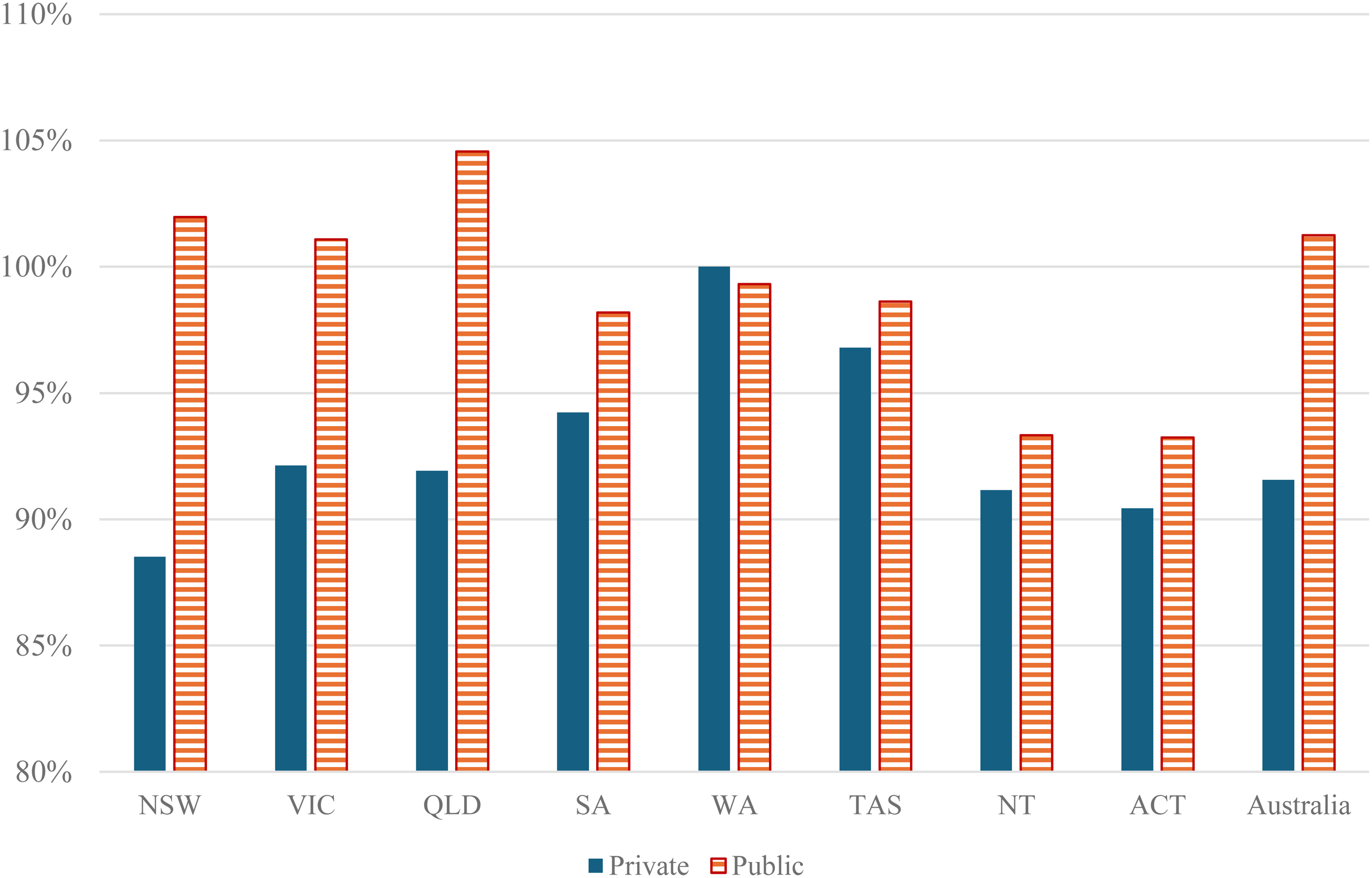
Wage growth in Australia, by state and sector, 2001–2023.

This paper has three main aims. The first, as noted, is to provide an updated analysis of public–private sector wage gaps in Australia (i.e., the gap nationally and the gap within and across states) (we do not offer a disaggregated analysis of the sector-wage differential within the Northern Territory (NT) or the Australian Capital Territory (ACT) on account of too few observations but we do include the NT and ACT samples in the national analysis). Our second aim is to understand how the public–private wage gap has evolved over the last two decades and whether there is any evidence of a particular trend which could be indicative of national rather than state-based wage effects. The third is to examine how the gap has evolved at the mean and across the wage distribution.

Approach

Various approaches may be adopted to measure the extent of the public–private sector wage gap, including techniques that examine the gap at the mean and the gap across the wage distribution.

Dummy variable approach

The simplest approach is to estimate a wage equation using ordinary least squares (OLS) and incorporate a dummy variable, ‘Public’, (coded as 1 if employed in the public sector and 0 if employed in the private sector) to capture the size and significance of the public-sector wage gap (i.e., gap after controlling for other factors thought to affect wages). Equation (1) illustrates such a model, with X being a vector of other characteristics thought to determine wages and $ε$ an error term.

\ln (W a g e_{i}) = P u b l i c_{i} β + X_{i} γ + ε_{i}

(1)

Blinder-Oaxaca decomposition approach

A variant on the ‘dummy variable approach’ in equation (1) is to use the Blinder-Oaxaca decomposition technique (Blinder, 1973; Oaxaca, 1973). The approach requires the estimation of separate regressions for public- and private-sector employees (equations (2) and (3)):

\ln ({Wage}_{pub, i}) = β_{Pub} X_{Pub, i} + ε_{Pub, i}

(2)

\ln ({Wage}_{Priv, i}) = β_{Priv} X_{Priv, i} + ε_{Priv, i}

(3)

After estimation, the subtraction of equation (3) from (2) and a rearrangement of terms we may express the Blinder-Oaxaca decomposition as follows:

\ln (gap) = ({\bar{X}}_{Pub} - {\bar{X}}_{Priv}) {\hat{β}}_{Pub} + {\bar{X}}_{Priv} ({\hat{β}}_{Pub} - {\hat{β}}_{Priv})

(4)

The first term on the right-hand side of equation (4) shows the share of the gap that arises from compositional differences in public- and private-sector workforces. The second term shows the share of the gap that arises from differences in the way that public- and private-sector workers’ characteristics are remunerated (‘coefficients’) and differences in the constants. Taken together, differences in the coefficients plus differences in the constants are commonly referred to as the unexplained component. Jones (1983) shows that the factors contributing to the size of the coefficients and size of the gap in the constants may vary with changes in the way the dummy variables are coded. The magnitude of the total unexplained share (the difference in the coefficients and the constants) together is not affected by the coding process. It could, however, be affected by the variables in the model. If relevant variables are not included in the model the unexplained component will capture discrimination as well as the effects of these omitted variables. Social or normative factors such as gender norms and gender stereotypes that affect decisions that correlate with wages (e.g., investment in education, time in the labour market), for example, will be captured in the unexplained term.

In the literature, there is some debate on whether to weight the decomposition using the public-sector or the private-sector wage structure (for a useful discussion, see Blinder, 1973 or Borland et al., 1998). It is not uncommon, however, to weight using the public-sector wage structure (e.g., Birch, 2006; Preston, 2001). Accordingly, we adopt this approach in this paper. Such an approach has the advantage of showing how much higher private-sector wages need to be (on average) to achieve parity with the public sector (under the assumption of a public-sector premium).

Panel estimators

With the increasing availability of longitudinal data, panel estimation techniques are now more commonly employed in studies of the public–private sector wage gap (e.g., Mahuteau et al., 2017). A preferred panel estimator is a fixed effects (FE) estimator given its value in capturing unobserved characteristics (e.g., ability, preferences for particular sectors, hours preferences etc.) that may be driving sector wage differences (Mahuteau et al., 2017). The FE approach also suffers from a number of limitations. For example, in the FE approach identification of the wage effect relies on those who change sectors. As will be shown below, the proportion of workers in Australia who switch sector of employment is relatively small. Between 2001 and 2022 around 10% of public-sector employees (nationally) switched from the public to the private sector. The share switching from the private sector to the public sector is even smaller (around 4.5%). This means that identification is based on a relatively small portion of the workforce that may have different characteristics to those who stay, leading to results that may not be representative of the entire population. The FE estimates may also be biased if there are unobserved factors that affect the decision to change jobs and affect wages. An example might be changes in human practices within firms.

In the analysis that follows there are sufficient observations to support an FE estimation approach at a national level and an FE approach within the larger states (NSW, VIC and Queensland [QLD]). In the smaller states the number of unique individuals is small, particularly when disaggregated by sector and by sex. For example, in TAS there are 131 unique individuals in the public sector during 2015–2022, with the share switching from the public to the private sector equal to 6.9% (see Table S1 in the online supplemental appendix). We, therefore, eschew a FE approach in these smaller states and, instead, use a random effects (RE) panel estimator. The advantage of the latter is that estimates of the sector-wage gap is based on variations within and across individuals. We recognise that the RE estimator requires the strict assumption that the unobservable characteristics are not correlated with the input variables and that this assumption is likely violated in this analysis. However, we also believe that the RE estimates are an improvement on the OLS estimates. The OLS and RE estimates presented in this paper should be seen as descriptive only.

Quantile approach

Mahuteau et al. (2017) uses a FE quantile regression model with a dummy variable controlling for sector of employment to examine how wages vary across the distribution. We similarly use an FE quantile approach to examine trends across the distribution. As will be noted, we confine this analysis to the national level only.

Time period

For most of the empirical findings we disaggregate the data into the two times periods: 2001–2014 (being the period reported in Mahuteau et al., 2017) and 2015–2022 (for the updated analysis). For the trend analysis, we examine the gap using a moving 5-year window (5-year panel) with FE and RE estimates reported at the national level and by state (as noted, for SA, WA and TAS we only report RE estimates). This trend analysis covers the period 2001–2022 (2001–2005; 2002–2006; 2003–2007; … 2018–2022). The quantile analysis similarly uses a 5-year moving window.

Data, variables, sample and descriptive statistics

Data and variables

The empirical work draws on data from the Household, Income and Labour Dynamics (HILDA) Survey. HILDA is a representative household panel survey that first commenced in 2001. At the time of writing there were 22 waves of data, covering 2001 to 2022. In the interest of building on Mahuteau et al. (2017) our decisions concerning the sample, regression models and variable construction closely follows their work. Our focus, therefore, is on employees aged 21 to 65 years, inclusive. Persons who are self-employed are excluded. The dependent variable is the natural logarithm hourly wage in the main job in 2022 prices. Hourly wages are derived as usual weekly wage in main job divided by usual weekly hours in main job.

Our main variable of interest is sector of employment. In HILDA, sector of employment is self-reported. Following Mahuteau et al. (2017), we classify those reporting that they work for a ‘private sector for profit organisation’ or a ‘private sector not for profit organisation’ as working in the private sector. Those reporting that they work for a ‘government business enterprise or commercial statutory authority’ or ‘other governmental organisation’ are classified as public-sector workers. A small (e.g., 0.8% from the initial 2001–2014 sample) report that they work in ‘other commercial’ and ‘other non-commercial’ sectors. These employees are excluded from the analysis.

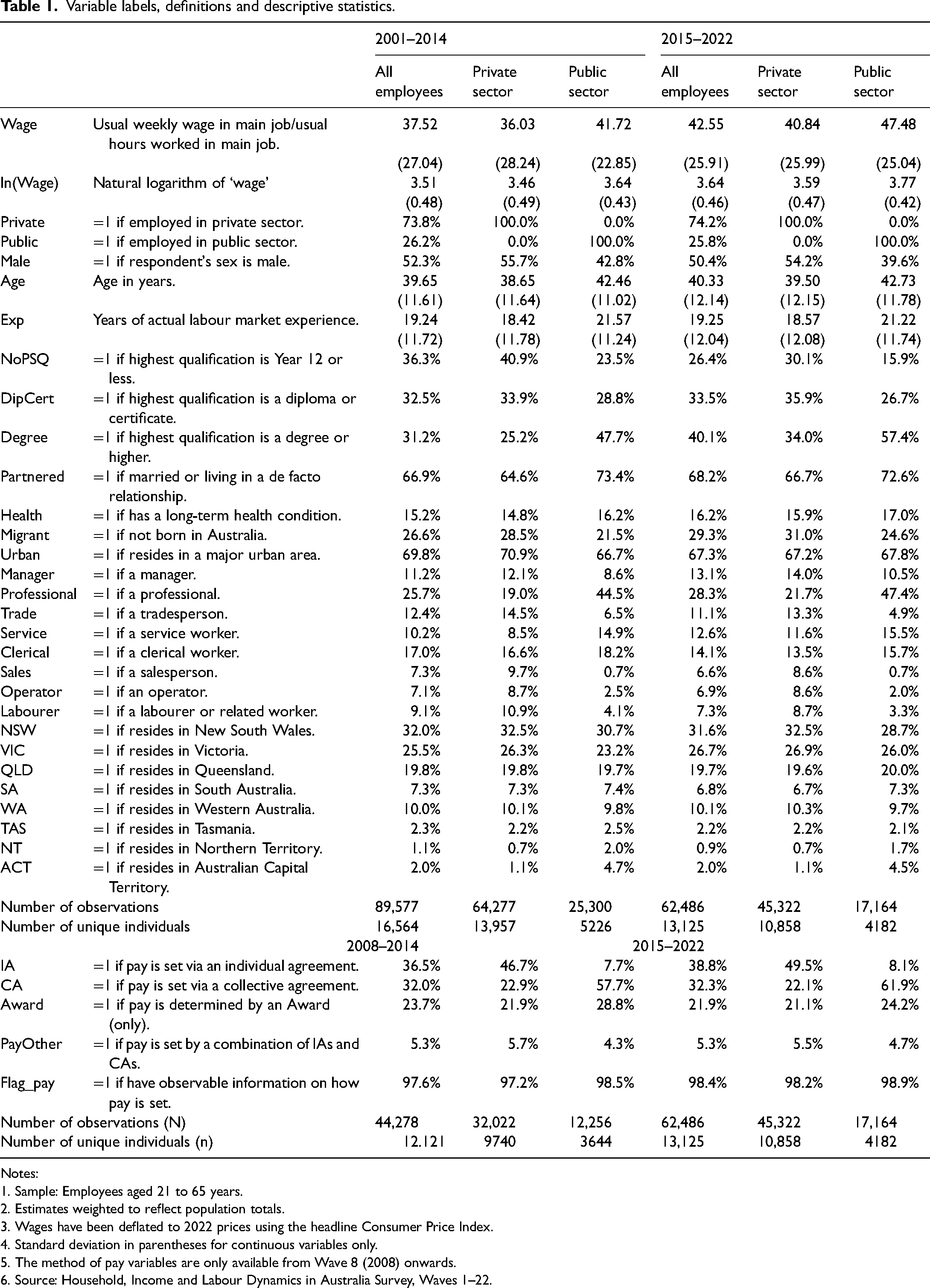
Table 1 details the construction of the variables used in the regressions. As indicated, we pay close attention to the specification used by Mahuteau et al. (2017) but with some modifications. Mahuteau et al. (2017) for example, would appear to model wages with age as a regressor. While we show the descriptives for age in Table 1, we use actual labour experience (‘Exp’) and its square in the regressions to be more consistent with human capital theory.

Table 1.

Variable labels, definitions and descriptive statistics.

		2001–2014			2015–2022
		All employees	Private sector	Public sector	All employees	Private sector	Public sector
Wage	Usual weekly wage in main job/usual hours worked in main job.	37.52	36.03	41.72	42.55	40.84	47.48
		(27.04)	(28.24)	(22.85)	(25.91)	(25.99)	(25.04)
ln(Wage)	Natural logarithm of ‘wage’	3.51	3.46	3.64	3.64	3.59	3.77
		(0.48)	(0.49)	(0.43)	(0.46)	(0.47)	(0.42)
Private	=1 if employed in private sector.	73.8%	100.0%	0.0%	74.2%	100.0%	0.0%
Public	=1 if employed in public sector.	26.2%	0.0%	100.0%	25.8%	0.0%	100.0%
Male	=1 if respondent's sex is male.	52.3%	55.7%	42.8%	50.4%	54.2%	39.6%
Age	Age in years.	39.65	38.65	42.46	40.33	39.50	42.73
		(11.61)	(11.64)	(11.02)	(12.14)	(12.15)	(11.78)
Exp	Years of actual labour market experience.	19.24	18.42	21.57	19.25	18.57	21.22
		(11.72)	(11.78)	(11.24)	(12.04)	(12.08)	(11.74)
NoPSQ	=1 if highest qualification is Year 12 or less.	36.3%	40.9%	23.5%	26.4%	30.1%	15.9%
DipCert	=1 if highest qualification is a diploma or certificate.	32.5%	33.9%	28.8%	33.5%	35.9%	26.7%
Degree	=1 if highest qualification is a degree or higher.	31.2%	25.2%	47.7%	40.1%	34.0%	57.4%
Partnered	=1 if married or living in a de facto relationship.	66.9%	64.6%	73.4%	68.2%	66.7%	72.6%
Health	=1 if has a long-term health condition.	15.2%	14.8%	16.2%	16.2%	15.9%	17.0%
Migrant	=1 if not born in Australia.	26.6%	28.5%	21.5%	29.3%	31.0%	24.6%
Urban	=1 if resides in a major urban area.	69.8%	70.9%	66.7%	67.3%	67.2%	67.8%
Manager	=1 if a manager.	11.2%	12.1%	8.6%	13.1%	14.0%	10.5%
Professional	=1 if a professional.	25.7%	19.0%	44.5%	28.3%	21.7%	47.4%
Trade	=1 if a tradesperson.	12.4%	14.5%	6.5%	11.1%	13.3%	4.9%
Service	=1 if a service worker.	10.2%	8.5%	14.9%	12.6%	11.6%	15.5%
Clerical	=1 if a clerical worker.	17.0%	16.6%	18.2%	14.1%	13.5%	15.7%
Sales	=1 if a salesperson.	7.3%	9.7%	0.7%	6.6%	8.6%	0.7%
Operator	=1 if an operator.	7.1%	8.7%	2.5%	6.9%	8.6%	2.0%
Labourer	=1 if a labourer or related worker.	9.1%	10.9%	4.1%	7.3%	8.7%	3.3%
NSW	=1 if resides in New South Wales.	32.0%	32.5%	30.7%	31.6%	32.5%	28.7%
VIC	=1 if resides in Victoria.	25.5%	26.3%	23.2%	26.7%	26.9%	26.0%
QLD	=1 if resides in Queensland.	19.8%	19.8%	19.7%	19.7%	19.6%	20.0%
SA	=1 if resides in South Australia.	7.3%	7.3%	7.4%	6.8%	6.7%	7.3%
WA	=1 if resides in Western Australia.	10.0%	10.1%	9.8%	10.1%	10.3%	9.7%
TAS	=1 if resides in Tasmania.	2.3%	2.2%	2.5%	2.2%	2.2%	2.1%
NT	=1 if resides in Northern Territory.	1.1%	0.7%	2.0%	0.9%	0.7%	1.7%
ACT	=1 if resides in Australian Capital Territory.	2.0%	1.1%	4.7%	2.0%	1.1%	4.5%
Number of observations		89,577	64,277	25,300	62,486	45,322	17,164
Number of unique individuals		16,564	13,957	5226	13,125	10,858	4182
		2008–2014			2015–2022
IA	=1 if pay is set via an individual agreement.	36.5%	46.7%	7.7%	38.8%	49.5%	8.1%
CA	=1 if pay is set via a collective agreement.	32.0%	22.9%	57.7%	32.3%	22.1%	61.9%
Award	=1 if pay is determined by an Award (only).	23.7%	21.9%	28.8%	21.9%	21.1%	24.2%
PayOther	=1 if pay is set by a combination of IAs and CAs.	5.3%	5.7%	4.3%	5.3%	5.5%	4.7%
Flag_pay	=1 if have observable information on how pay is set.	97.6%	97.2%	98.5%	98.4%	98.2%	98.9%
Number of observations (N)		44,278	32,022	12,256	62,486	45,322	17,164
Number of unique individuals (n)		12.121	9740	3644	13,125	10,858	4182

Notes:

1. Sample: Employees aged 21 to 65 years.

2. Estimates weighted to reflect population totals.

3. Wages have been deflated to 2022 prices using the headline Consumer Price Index.

4. Standard deviation in parentheses for continuous variables only.

5. The method of pay variables are only available from Wave 8 (2008) onwards.

6. Source: Household, Income and Labour Dynamics in Australia Survey, Waves 1–22.

There is some debate in the literature as to whether occupation should be controlled for when estimating the public-sector wage differentials (Belman and Heywood, 2004). The case for including occupation is that it may capture particular characteristics (skills or abilities) of an occupation that are unique to the public sector and which ‘explain’ sector wage differences. However, it is also the case that there are particular occupations which are overrepresented in the public sector (e.g., professionals) and underrepresented in the private sector. Controlling for occupation may cause the size of the public–private sector wage gap to be understated. In the analysis below we, therefore, explore the results with and without occupation controls. Mahuteau et al. (2017) include occupation (one-digit) controls in their analysis.

We also deviate slightly from Mahuteau et al. (2017) via the incorporation of controls for method of pay setting (for periods when this information is available). Beginning in 2008 (Wave 8), the HILDA Survey incorporated questions on method of pay setting (Collective Agreement [CA], Individual Arrangement [IA], Award [Award] or other [PayOther]). As shown in Table 1, pay setting arrangements differ markedly between the public and private sectors. In the 2015–2022 period, for example, 61.9% of public-sector employees had their pay set by a CA. In the private sector, the share was 22.1%. As information on pay setting is only available from 2008, we do not include these controls in the analysis comparing wage differentials over the full period of 2001 to 2022 period (i.e., the trend analysis).

Sample

To give a perspective of the representative nature of the sample, we describe the starting sample size and eventual sample size (the working sample) associated with the 2001–2014 period. In total, in the 2001–2014 period, there are 91,769 observations who are employees and who are aged 21–65 years and work in either the public or private sector (and not in other commercial or other non-commercial workplaces). After excluding observations who were technically employed but did not receive a wage (had zero earnings in the survey week, perhaps because they were on unpaid leave) or were missing information on either occupation, education, marital status, birthplace, or state of residence, we lose 976 observations or 1% of the sample. This reduces the sample to 90,793 observations. We drop a further 1216 observations (1.3% of the 90,793 sample) on account of missing information on actual labour market experience (an important variable in the wage equation). Our working sample for the 2001–2014 period contains 89,577 observations or 16,564 persons (unique individuals). Using the same sample selection rules the working sample for the 2015–2022 period is 62,486 observations or 13,125 persons. During 2001–2014, 26.2% of observations were employed in the public sector. During 2015–2022, the proportion was 25.8%.

Table S1 in the online supplemental appendix provides select panel descriptives. The prime aim of this table is to show the number of persons (unique individuals) by sector and state and the number who switch sectors. Most employees are not sector movers. On average only 10% of public-sector workers switched to the private sector and an even smaller share (5%) of private-sector workers switched to the public sector. The mean number of waves that an individual is observed over was 5.4 in the 2001–2014 period and 4.8 in the 2015–2022 period. This lends further support to the 5-year moving window approach employed when examining trends in the gap.

Descriptive statistics

Descriptive statistics are reported in Table 1. The raw public–private sector gap, in percentage terms is equal to 15.8% during 2001–2014 and 16.3% during 2015–2022.³ The estimates also show that when compared to private-sector employees, public-sector employees are older, have higher levels of labour market experience, are more qualified, more likely to be married, more likely to have a long-term health condition, and less likely to have been born overseas. In the 2015–2022 period, the share of public-sector employees with a degree had increased to 57.4% (up from 47.7% during 2001–2014) while the share of degree qualified private-sector employees was equal to 34.0% (up from 25.3% during 2001–2014).

The occupational data shows that there is a disproportionate share of professionals (e.g., teachers, nurses etc.) in the public sector. During 2001–2014, nearly half (44.5%) of public-sector employees were professionals. During 2015–2022, this share had increased to 47.4%, likely reflecting the expansion of the health and education sectors over the period. Other occupations such as salespersons, operators and labourers are underrepresented in the public sector. The estimates also show that men are underrepresented in the public sector (or that women are overrepresented). During 2001–2014, 42.8% of public-sector employees were men. By 2015–2022, this share had fallen to 39.6%.

In the bottom panel of Table 1 we report the summary statistics for the method of pay setting variables. As previously noted, this information is only available from 2008 in HILDA. We see no reason to restate all the descriptive information for all other variables for the 2008–14 period. Our main purpose in this bottom panel is to simply show that pay setting arrangements differ between the public and private sectors. In the period after 2014, IAs have become more prevalent while the share dependent only on the Award has decreased.

Results

The public–private sector wage gap at the mean—using the dummy variable approach

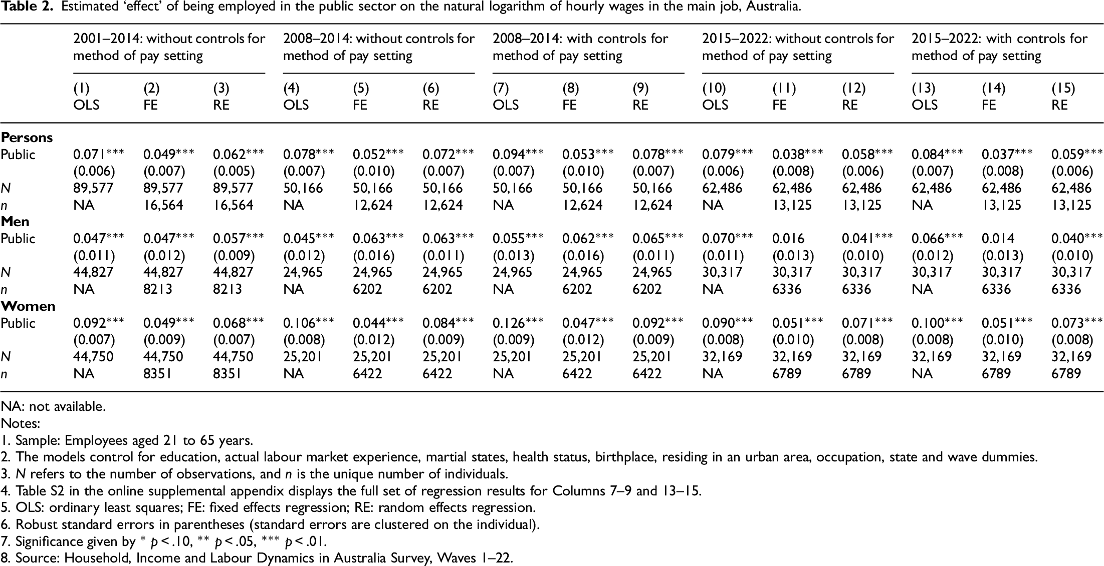
Table 2 displays the estimated public–private wage gap using the dummy variable approach. Three sets of estimates are provided for each time period shown: (a) using OLS; (b) using a FE panel estimator; and (c) using an RE panel estimator. We also disaggregate the analysis by sex and provide estimates with and without the pay-setting controls (in order that comparisons may also be made back to Mahuteau et al. and to periods prior to when this data was available). The results presented are from models with controls for occupation.

Table 2.

Estimated ‘effect’ of being employed in the public sector on the natural logarithm of hourly wages in the main job, Australia.

	2001–2014: without controls for method of pay setting			2008–2014: without controls for method of pay setting			2008–2014: with controls for method of pay setting			2015–2022: without controls for method of pay setting			2015–2022: with controls for method of pay setting
	(1)	(2)	(3)	(4)	(5)	(6)	(7)	(8)	(9)	(10)	(11)	(12)	(13)	(14)	(15)
	OLS	FE	RE	OLS	FE	RE	OLS	FE	RE	OLS	FE	RE	OLS	FE	RE
Persons
Public	0.071***	0.049***	0.062***	0.078***	0.052***	0.072***	0.094***	0.053***	0.078***	0.079***	0.038***	0.058***	0.084***	0.037***	0.059***
	(0.006)	(0.007)	(0.005)	(0.007)	(0.010)	(0.007)	(0.007)	(0.010)	(0.007)	(0.006)	(0.008)	(0.006)	(0.007)	(0.008)	(0.006)
N	89,577	89,577	89,577	50,166	50,166	50,166	50,166	50,166	50,166	62,486	62,486	62,486	62,486	62,486	62,486
n	NA	16,564	16,564	NA	12,624	12,624	NA	12,624	12,624	NA	13,125	13,125	NA	13,125	13,125
Men
Public	0.047***	0.047***	0.057***	0.045***	0.063***	0.063***	0.055***	0.062***	0.065***	0.070***	0.016	0.041***	0.066***	0.014	0.040***
	(0.011)	(0.012)	(0.009)	(0.012)	(0.016)	(0.011)	(0.013)	(0.016)	(0.011)	(0.011)	(0.013)	(0.010)	(0.012)	(0.013)	(0.010)
N	44,827	44,827	44,827	24,965	24,965	24,965	24,965	24,965	24,965	30,317	30,317	30,317	30,317	30,317	30,317
n	NA	8213	8213	NA	6202	6202	NA	6202	6202	NA	6336	6336	NA	6336	6336
Women
Public	0.092***	0.049***	0.068***	0.106***	0.044***	0.084***	0.126***	0.047***	0.092***	0.090***	0.051***	0.071***	0.100***	0.051***	0.073***
	(0.007)	(0.009)	(0.007)	(0.008)	(0.012)	(0.009)	(0.009)	(0.012)	(0.009)	(0.008)	(0.010)	(0.008)	(0.008)	(0.010)	(0.008)
N	44,750	44,750	44,750	25,201	25,201	25,201	25,201	25,201	25,201	32,169	32,169	32,169	32,169	32,169	32,169
n	NA	8351	8351	NA	6422	6422	NA	6422	6422	NA	6789	6789	NA	6789	6789

NA: not available.

Notes:

1. Sample: Employees aged 21 to 65 years.

2. The models control for education, actual labour market experience, martial states, health status, birthplace, residing in an urban area, occupation, state and wave dummies.

3. N refers to the number of observations, and n is the unique number of individuals.

4. Table S2 in the online supplemental appendix displays the full set of regression results for Columns 7–9 and 13–15.

5. OLS: ordinary least squares; FE: fixed effects regression; RE: random effects regression.

6. Robust standard errors in parentheses (standard errors are clustered on the individual).

7. Significance given by * p < .10, ** p < .05, *** p < .01.

8. Source: Household, Income and Labour Dynamics in Australia Survey, Waves 1–22.

Focusing on Column a (for 2001–2014) for persons (and for models without pay setting controls), the coefficient from the OLS regression for working in the public sector is equal to 0.071. When expressed as a percentage, this shows that there is a public-sector premium equal to 7.4% (computed as: [exp(0.071)−1]×100) based on the Halvorsen and Palmquist (1980) approach for interpreting dummy variables in linear wage models. All marginal effects discussed in the body of the paper have been calculated using this method. Mahuteau et al. (2017) similarly report a public-sector wage gap of 7.4% in their 2001–2014 pooled OLS estimates. This, of course, is comforting as we have deliberately followed Mahuteau et al. (2017) in terms of choice of working sample and model specification (other than the variable to capture labour market experience), although we do have a slightly larger sample. Our FE estimates (Column 2) show that public-sector employees during 2001–2014, on average, earned 5.0% more than private-sector employees and that there was little difference in the size of the public-sector premium by gender.

The estimates in Column 2 may be compared to the estimates in Column 11. When we do this, we see that the observed 5% public-sector wage premium during 2001–2014 fell to 3.9% during 2015–2022. The interesting result, however, is in the disaggregated estimates. During 2001–2014 the public-sector wage premium among men was equal to 4.8% and was highly statistically significant. By 2015–2022 it had fallen to 1.6% and was insignificant. Among women the public-sector premium was equal to 5% during 2001–2014, and by 2015–2022, it was marginally higher at 5.2%. In both cases it was highly statistically significant. In other words, in the 2015–2022 period the observed public-sector wage premium is being driven by outcomes in the female labour market. The increase may stem from policies directed at improving gender equality in the public sector (Jean and Groves, 2024 ; Workplace Gender Equality Agency [WGEA], 2023).⁴

State public–private sector wage gaps at the mean—dummy variable approach

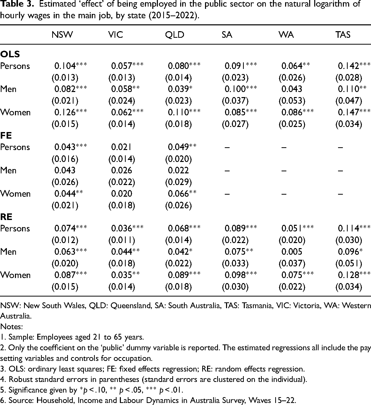
Table 3 displays the OLS, FE and RE coefficient estimates disaggregated by state. We only present results for the 2015–2022 period as our interest is in understanding the extent to which the gap differs (if at all) within states. As previously noted, we do not present estimates for the territories on account of data limitations.

Table 3.

Estimated ‘effect’ of being employed in the public sector on the natural logarithm of hourly wages in the main job, by state (2015–2022).

	NSW	VIC	QLD	SA	WA	TAS
OLS
Persons	0.104***	0.057***	0.080***	0.091***	0.064**	0.142***
	(0.013)	(0.013)	(0.014)	(0.023)	(0.026)	(0.028)
Men	0.082***	0.058**	0.039*	0.100***	0.043	0.110**
	(0.021)	(0.024)	(0.023)	(0.037)	(0.053)	(0.047)
Women	0.126***	0.062***	0.110***	0.085***	0.086***	0.147***
	(0.015)	(0.014)	(0.018)	(0.027)	(0.025)	(0.034)
FE
Persons	0.043***	0.021	0.049**	–	–	–
	(0.016)	(0.014)	(0.020)
Men	0.043	0.026	0.022	–	–	–
	(0.026)	(0.022)	(0.029)
Women	0.044**	0.020	0.066**	–	–	–
	(0.021)	(0.018)	(0.026)
RE
Persons	0.074***	0.036***	0.068***	0.089***	0.051***	0.114***
	(0.012)	(0.011)	(0.014)	(0.022)	(0.020)	(0.030)
Men	0.063***	0.044**	0.042*	0.075**	0.005	0.096*
	(0.020)	(0.018)	(0.022)	(0.033)	(0.037)	(0.051)
Women	0.087***	0.035**	0.089***	0.098***	0.075***	0.128***
	(0.015)	(0.014)	(0.018)	(0.030)	(0.022)	(0.034)

NSW: New South Wales, QLD: Queensland, SA: South Australia, TAS: Tasmania, VIC: Victoria, WA: Western Australia.

Notes:

1. Sample: Employees aged 21 to 65 years.

2. Only the coefficient on the ‘public’ dummy variable is reported. The estimated regressions all include the pay setting variables and controls for occupation.

3. OLS: ordinary least squares; FE: fixed effects regression; RE: random effects regression.

4. Robust standard errors in parentheses (standard errors are clustered on the individual).

5. Significance given by *p < .10, ** p < .05, *** p < .01.

6. Source: Household, Income and Labour Dynamics in Australia Survey, Waves 15–22.

For the larger states, we focus our discussion on the FE results as we believe the samples are sufficiently large in NSW, VIC and QLD to support an FE analysis. In each of these states in the 2015–2022 period, there are, respectively, 1143, 1149 and 851 persons (unique employees) who work in the public sector. The average share switching sector (from public to private) is around 10%. In the smaller states our analysis is descriptive, based on the RE results (in SA, WA and TAS, there are only 379, 377 and 371 unique employees, respectively. The switching shares are 10.3%, 9.8% and 6.9%, respectively) (see Table S1 in the online supplemental appendix).

We first discuss the FE estimates for NSW, VIC and QLD. A common finding (and one that is in keeping with the national estimates) is that there is no evidence of a public–private-sector wage gap among men. Indeed, for VIC, there is no evidence of a public–private-sector wage gap for men or women. In NSW and QLD, the public–private sector wage gap is driven by the public-sector wage premiums among women. In the former this premium for women is equal to 4.5%. In QLD the corresponding premium is 6.8%. These wage premiums again may be capturing initiatives to improve gender wage equality in these states. For example, in 2016, the QLD Government initiated the ‘Queensland Women's Strategy 2016–2021’ with several policies aimed at improving gender pay equality in the state and many initiatives directed to women in the public sector (see Office for Women, 2024). Indeed, the Office of the Special Commissioner, Equity and Diversity (2023) shows that gender wage gap in the public sector for QLD narrowed since 2015 and was much smaller than the gap for the public sector at a national level.

The RE estimates in the remaining states (SA, WA and TAS) similarly show that the public–private sector premium in these states is driven by outcomes among women. The RE estimates point to a particularly large public–private sector wage premium for women in TAS. Mahuteau et al. (2017) similarly found a larger public-sector premium among women in TAS and suggested that it might reflect the use of a premium to attract and retain public-sector workers in TAS.

A key feature of the results is the extent to which the public–private sector earnings gap varies by state (a similar finding was reported in Mahuteau et al., 2017). We suggest that this may mean that state-level wage-setting forces are more influential than national ones. In other words, local labour markets are more important when it comes to considering sector wage differences.

Blinder-Oaxaca decomposition—what's driving the sector-wage gaps?

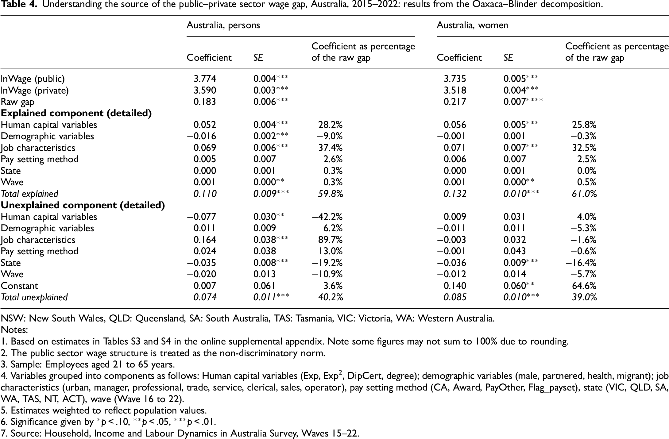
Table 4 displays the results associated with a decomposition of the public–private sector wage gap nationally using the Oaxaca–Blinder technique (Tables S3 and S4 in the online supplemental appendix show the means and regression output used in the decomposition of the gap nationally). Two sets of estimates are reported. The first is for persons (men and women pooled) and the second is for women only (given that the gap is primarily driven by outcomes among women).

Table 4.

Understanding the source of the public–private sector wage gap, Australia, 2015–2022: results from the Oaxaca–Blinder decomposition.

	Australia, persons			Australia, women
	Coefficient	SE	Coefficient as percentage of the raw gap	Coefficient	SE	Coefficient as percentage of the raw gap
lnWage (public)	3.774	0.004***		3.735	0.005***
lnWage (private)	3.590	0.003***		3.518	0.004***
Raw gap	0.183	0.006***		0.217	0.007****
Explained component (detailed)
Human capital variables	0.052	0.004***	28.2%	0.056	0.005***	25.8%
Demographic variables	−0.016	0.002***	−9.0%	−0.001	0.001	−0.3%
Job characteristics	0.069	0.006***	37.4%	0.071	0.007***	32.5%
Pay setting method	0.005	0.007	2.6%	0.006	0.007	2.5%
State	0.000	0.001	0.3%	0.000	0.001	0.0%
Wave	0.001	0.000**	0.3%	0.001	0.000**	0.5%
Total explained	0.110	0.009***	59.8%	0.132	0.010***	61.0%
Unexplained component (detailed)
Human capital variables	−0.077	0.030**	−42.2%	0.009	0.031	4.0%
Demographic variables	0.011	0.009	6.2%	−0.011	0.011	−5.3%
Job characteristics	0.164	0.038***	89.7%	−0.003	0.032	−1.6%
Pay setting method	0.024	0.038	13.0%	−0.001	0.043	−0.6%
State	−0.035	0.008***	−19.2%	−0.036	0.009***	−16.4%
Wave	−0.020	0.013	−10.9%	−0.012	0.014	−5.7%
Constant	0.007	0.061	3.6%	0.140	0.060**	64.6%
Total unexplained	0.074	0.011***	40.2%	0.085	0.010***	39.0%

NSW: New South Wales, QLD: Queensland, SA: South Australia, TAS: Tasmania, VIC: Victoria, WA: Western Australia.

Notes:

1. Based on estimates in Tables S3 and S4 in the online supplemental appendix. Note some figures may not sum to 100% due to rounding.

2. The public sector wage structure is treated as the non-discriminatory norm.

3. Sample: Employees aged 21 to 65 years.

4. Variables grouped into components as follows: Human capital variables (Exp, Exp², DipCert, degree); demographic variables (male, partnered, health, migrant); job characteristics (urban, manager, professional, trade, service, clerical, sales, operator), pay setting method (CA, Award, PayOther, Flag_payset), state (VIC, QLD, SA, WA, TAS, NT, ACT), wave (Wave 16 to 22).

5. Estimates weighted to reflect population values.

6. Significance given by *p < .10, **p < .05, ***p < .01.

7. Source: Household, Income and Labour Dynamics in Australia Survey, Waves 15–22.

Focusing on the results for women, the estimates show that the raw public–private sector wage gap is equal to 0.217 log points. Of this gap 0.132 log points (or 61.0%) may be explained by differences in the characteristics of women who are public- and private-sector employees. At a disaggregated level we see that 32.5% of the raw gap arises from sectoral differences in the jobs (occupations) that women hold. As previously noted (and shown in the descriptive statistics in Table S3 in the online supplemental appendix) women in the public sector are more likely to be employed in higher paid occupations than those in the private sector. For example, during 2015–22, 53.7% of women in the public sector were Professionals, compared with 24.1% of women in the private sector. An additional 25.8% of the observed raw gap stems from differences in the human capital characteristics (education and experience) of women employed in the public and private sectors. During 2015–2022, 62.2% of women in the public sector had a degree. This compares to 36.9% of women in the private sector (Table S3 in the online supplemental appendix).

With 61% of the raw public–private sector wage gap among women explained by differences in the observed characteristics of public- and private-sector employees, this means 39% of the gap (the residual) is unexplained. The unexplained gap reflects sectorial treatment effects (i.e., differences in the way the sectors reward characteristics such as education and experience) and other factors not controlled for in the regression, including unobservable factors such as ability.

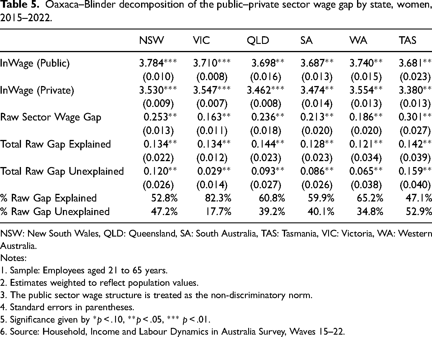
Table 5 summaries the Oaxaca–Blinder decomposition estimates for each of the six states for women. We focus on women rather than persons on account of our earlier analysis showing that the 2015–22 public-sector wage premium is being driven by women. Our main interest lies in understanding how much of the observed raw gap may be ‘explained’ (or described) by differences in characteristics. As shown, there is considerable heterogeneity in the explained share across states. In NSW, for example, the explained share is equal to 52.8%. In VIC it is equal to 82.3% and in QLD it is 60.8%. The explained share also varies across the smaller states, ranging from 47.1% in TAS to 65.2% in WA. For most states, the main source of the explained gap is differences in human capital (education, labour market experience) and occupation (results not reported but available on request). We believe this large variation in both the size of the raw public-sector wage gap and in the source of the gap lends additional support for our contention that public-sector wage gaps are locally driven.

Table 5.

Oaxaca–Blinder decomposition of the public–private sector wage gap by state, women, 2015–2022.

	NSW	VIC	QLD	SA	WA	TAS
lnWage (Public)	3.784***(0.010)	3.710***(0.008)	3.698**(0.016)	3.687**(0.013)	3.740**(0.015)	3.681**(0.023)
lnWage (Private)	3.530***(0.009)	3.547***(0.007)	3.462***(0.008)	3.474**(0.014)	3.554**(0.013)	3.380**(0.013)
Raw Sector Wage Gap	0.253**(0.013)	0.163**(0.011)	0.236**(0.018)	0.213**(0.020)	0.186**(0.020)	0.301**(0.027)
Total Raw Gap Explained	0.134**(0.022)	0.134**(0.012)	0.144**(0.023)	0.128**(0.023)	0.121**(0.034)	0.142**(0.039)
Total Raw Gap Unexplained	0.120**(0.026)	0.029**(0.014)	0.093**(0.027)	0.086**(0.026)	0.065**(0.038)	0.159**(0.040)
% Raw Gap Explained	52.8%	82.3%	60.8%	59.9%	65.2%	47.1%
% Raw Gap Unexplained	47.2%	17.7%	39.2%	40.1%	34.8%	52.9%

NSW: New South Wales, QLD: Queensland, SA: South Australia, TAS: Tasmania, VIC: Victoria, WA: Western Australia.

Notes:

1. Sample: Employees aged 21 to 65 years.

2. Estimates weighted to reflect population values.

3. The public sector wage structure is treated as the non-discriminatory norm.

4. Standard errors in parentheses.

5. Significance given by *p < .10, **p < .05, *** p < .01.

6. Source: Household, Income and Labour Dynamics in Australia Survey, Waves 15–22.

National and state public–private sector wage gaps across the wage distribution

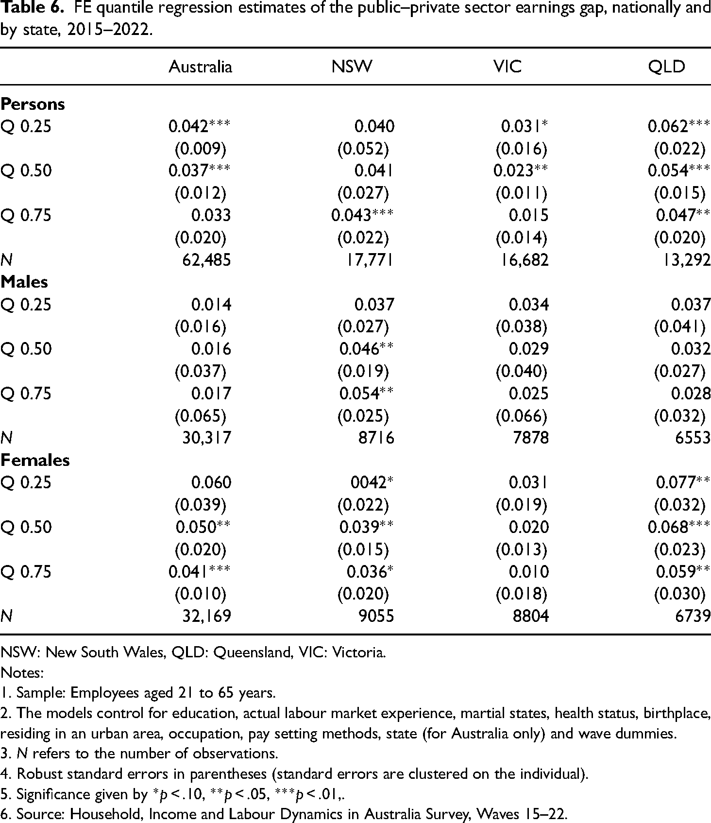
In Table 6 we present the quantile results. The focus is on the period of 2015–2022, and we consider quantiles 0.25 (low-paid workers), 0.50 (median-paid workers) and 0.75 (high-paid workers). Mahuteau et al. (2017) find statistically significant public sector earnings premiums at these quantiles for both men and women, with the premium being larger for low-paid workers and for women. As the estimates are from an FE estimator we only report results for Australia and for the large states (NSW, VIC and QLD).

Table 6.

FE quantile regression estimates of the public–private sector earnings gap, nationally and by state, 2015–2022.

	Australia	NSW	VIC	QLD
Persons
Q 0.25	0.042***(0.009)	0.040(0.052)	0.031*(0.016)	0.062***(0.022)
Q 0.50	0.037***(0.012)	0.041(0.027)	0.023**(0.011)	0.054***(0.015)
Q 0.75	0.033(0.020)	0.043***(0.022)	0.015(0.014)	0.047**(0.020)
N	62,485	17,771	16,682	13,292
Males
Q 0.25	0.014(0.016)	0.037(0.027)	0.034(0.038)	0.037(0.041)
Q 0.50	0.016(0.037)	0.046**(0.019)	0.029(0.040)	0.032(0.027)
Q 0.75	0.017(0.065)	0.054**(0.025)	0.025(0.066)	0.028(0.032)
N	30,317	8716	7878	6553
Females
Q 0.25	0.060(0.039)	0042*(0.022)	0.031(0.019)	0.077**(0.032)
Q 0.50	0.050**(0.020)	0.039**(0.015)	0.020(0.013)	0.068***(0.023)
Q 0.75	0.041***(0.010)	0.036*(0.020)	0.010(0.018)	0.059**(0.030)
N	32,169	9055	8804	6739

NSW: New South Wales, QLD: Queensland, VIC: Victoria.

Notes:

1. Sample: Employees aged 21 to 65 years.

2. The models control for education, actual labour market experience, martial states, health status, birthplace, residing in an urban area, occupation, pay setting methods, state (for Australia only) and wave dummies.

3. N refers to the number of observations.

4. Robust standard errors in parentheses (standard errors are clustered on the individual).

5. Significance given by *p < .10, **p < .05, ***p < .01,.

6. Source: Household, Income and Labour Dynamics in Australia Survey, Waves 15–22.

Focusing on the national results (Column 1), here we again see that across the distribution the public–private sector wage gap is driven by outcomes among women. The premium is smaller for high-paid women (estimated coefficient of 0.041 at quantile 0.75) than at the median (coefficient of 0.50 at quantile 0.50). There is no statistically significant difference in the sector wages of low-paid women. This finding contrasts with the finding Mahuteau et al. (2017) where they argue that the public-sector favours low-waged workers. Evidence here shows that it is highly skilled women who benefit from public sector employment.

Among men, there is no evidence of a public-sector wage premium across the distribution (as given by the insignificant coefficients). This result could imply that since the Mahuteau et al. (2017) study, the wages of males in the private sector have caught up with those in the public sector.

The disaggregated analysis by state (NSW, VIC and QLD) shows that again, most of the public–private sector wage differential is in the female labour market. Only high-paid men in NSW have a public-sector wage premium. In VIC and QLD there is no evidence of a sector-wage differential among men along the wage distribution.

Among women there is evidence of a sector-premium along the distribution, however, there is no specific pattern. In VIC there is no premium across the distribution (similar to men). In NSW and QLD a public-sector premium is observed at all points of the distribution studied, although it is markedly higher and statistically more significant in QLD.

Robustness checks

Before moving to the trend analysis of the public–private sector wage gap, we first conduct some robustness checks. The first examines the results when occupation is not controlled for in the wage model. The second considers results using a dependent variable that is trimmed (that is, the top and bottom 1% of the wage distribution are excluded from the sample). Finally, we examine the results when we also take into consideration Covid-19. The detailed findings associated with these checks are contained in the online supplemental appendix and are summarised below. The robustness checks are based on wages at the mean.

Without occupation

Our robustness checks reveals that the OLS estimates are significantly larger when occupation is removed. The removal of occupation, however, has only a marginal impact on the FE and the RE estimates. For example, during 2015–2022, Table 2 shows that, at the mean, the public–private sector earnings gap is equal to 3.8% using an FE estimator. This rises to 4.1% when occupation is removed (Table S6, Column 14, in the online supplemental appendix). When the sample is restricted to women, the FE estimates show that with occupation the premium is 5.2% (Table 2, Column 14) and without occupation it is 5.6% (Table S6, Column 14, in the online supplemental appendix). A similar pattern is found when disaggregating the results by state (see Table S7 in the online supplemental appendix).

Our next check considers the effects when we exclude the bottom and top 1% of the hourly wage (main job) distribution from the working sample. The results are summarised in Table S11 in the online supplemental appendix. In brief, removing these potential outliers makes little difference to the estimated public–private sector wage gaps. For example, prior to trimming the sample the public-sector premium among women during 2015–2022 is equal to 5.2% (Table 2, Column 14) using an FE estimator. After trimming this gap increases to 5.7% (Table S11, Column 5, in the online supplemental appendix).

Our final check considers the effect that Covid-19 may have had on the public–private sector wage gap. In the 2021 and 2022 HILDA survey respondents are asked whether they received any Covid-19 related payment in the previous financial year. We use this information to construct a binary variable (‘Covid’) coded as 1 if a payment was received and 0 otherwise. The robustness check is constrained to these two waves. The results are contained in Tables S12 and S13 in the online supplemental appendix. We first estimate a pooled model for the two waves without controlling for Covid and then repeat the exercise with the Covid dummy variable included. Based on the FE results (and for the full sample), when the model is estimated without this ‘Covid’ dummy variable, the coefficient on ‘Public’ is equal to 0.062. When ‘Covid’ is included, this coefficient falls to 0.061. The same pattern occurs for women (Table S13 in the online supplemental appendix). When ‘Covid’ is not included the coefficient on ‘Public’ is equal to 0.066 and when it is included the coefficient remains at 0.066. We conclude from this that our results are not sensitive to possible Covid effects.

Based on these checks the remainder of this paper proceeds with an analysis that includes an untrimmed dependent variable, a specification that includes 1-digit occupation controls and a specification that does not adjust for potential Covid-19 effects.

Trends in the public–private sector wage gap—nationally and by state

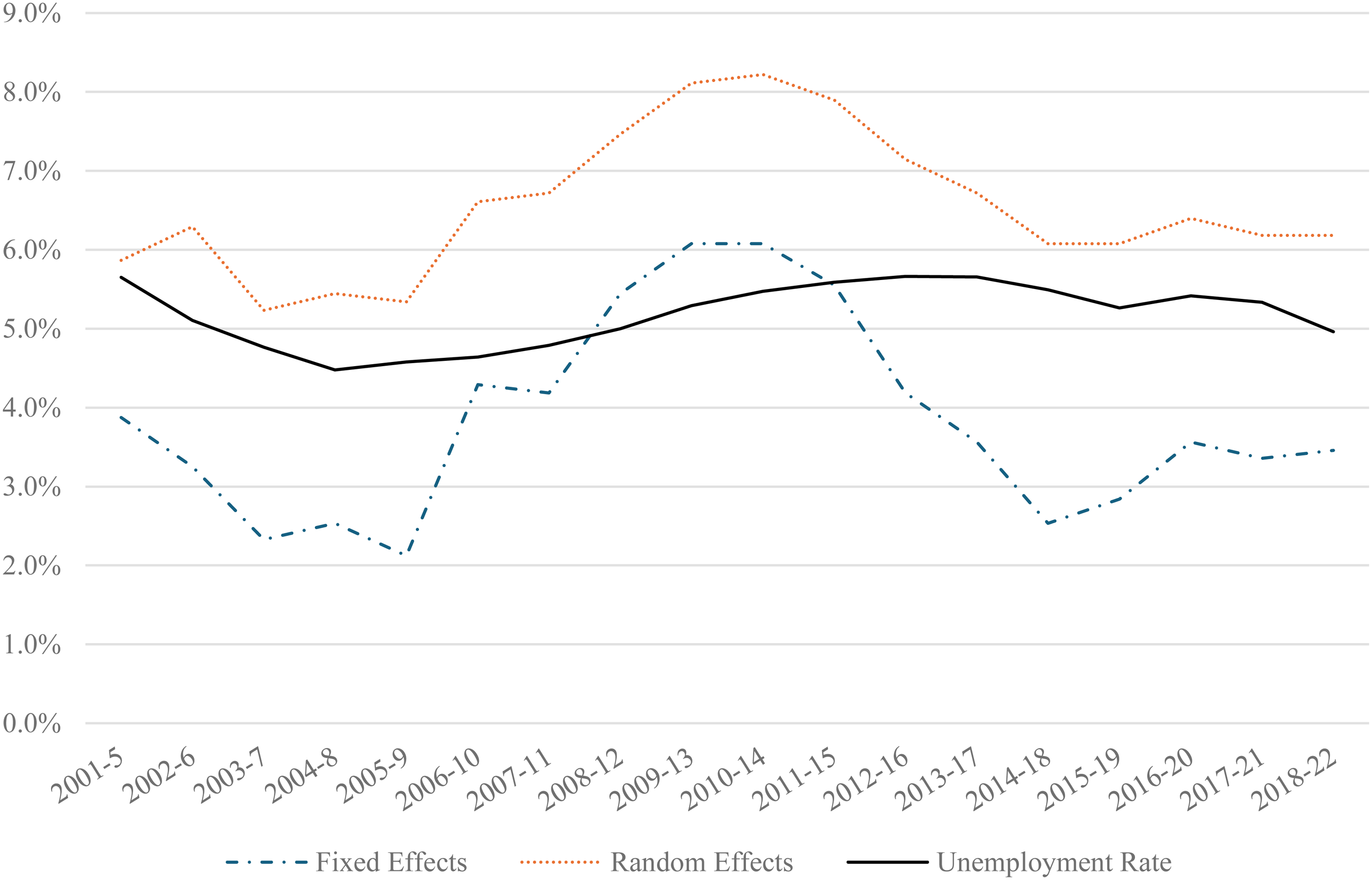
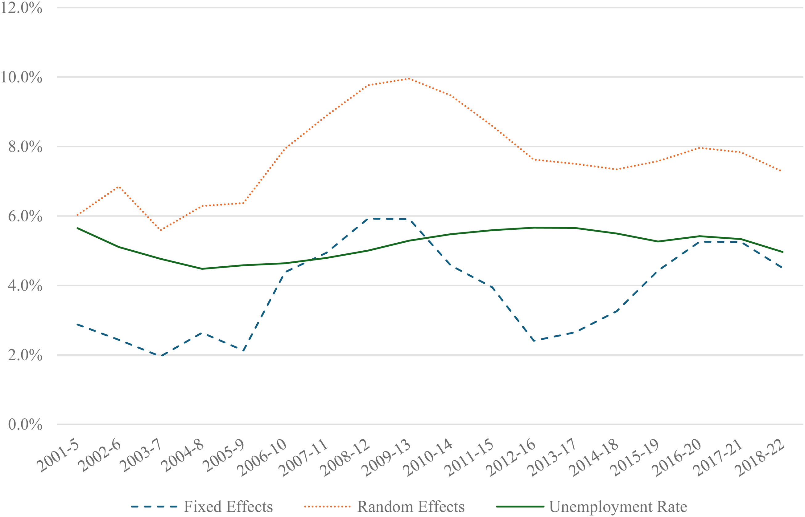
Figure 2 illustrates the trends in the public–private sector wage gap across Australia, with estimates derived using both FE and RE panel estimators over a rolling 5-year window. The sample includes both men and women. The RE and FE estimates are highly correlated, with a correlation coefficient of 0.95. Consistent with previous analyses, the wage gap estimated using the RE method is larger than when the FE method is applied. Focusing on the FE estimates, we observe that the wage gap decreased over the first five of the 5-year windows (2001–2005 to 2005–2009). It then increased from 2006–2010, peaking around 2010–2014, before sharply declining and reaching a low point around 2014–2018. The gap appears to have stabilised during the 2016–2020 period.

Figure 2.

Trends in the public–private sector wage gap in Australia, 2001–2005 to 2018–2022.

At a national level the gap appears to be neither procyclical nor countercyclical (based on a simple comparison with the observed national unemployment rate in the same window). Over the whole period shown the correlation coefficient, comparing the FE estimates with the unemployment rate, is equal to 0.36. If we restrict the period to 2001 to 2014 the FE and unemployment rate correlation coefficient rises to 0.60. It is clear from Figure 2 that the public–private sector wage gap and the unemployment rate had a much weaker correlation after 2014 than before. Figure 3 presents the results for women only. The pattern is similar to that shown in Figure 2 (for persons) (which is not surprising given earlier analysis suggesting that the public-sector gap is driven by outcomes in the female labour market).

Figure 3.

Trends in the public–private sector wage gap in Australia, 2001–2005 to 2018–2022, females.

Figures 4 shows trends in the public–private sector person wage gap at a state level (NSW, VIC and QLD) based on FE estimates. Figure 5 (for NSW, VIC and QLD) and Figure 6 (for SA, WA and TAS) show trends in the gap using an RE estimator. As noted previously, the trend estimates using the RE and FE estimators are highly correlated. Thus while the RE estimator may upwardly bias the premium associated with public-sector employment, they estimates are, nevertheless, valuable when it comes to observing trends (particularly across the smaller states). The corresponding estimates for females from the trend analysis by state are presented in Figures S1 to S3 in the online supplemental appendix, with detailed results (coefficients) reported in Table S13 in the online supplemental appendix.

Figure 4.

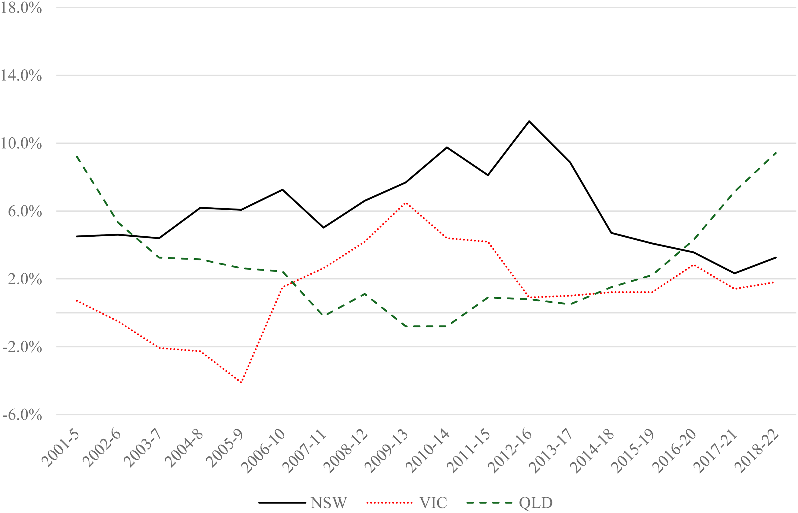
Fixed effects estimates of trends in the public–private sector wage gap in NSW, VIC and QLD 2001–2005 to 2018–2022.

Figure 5.

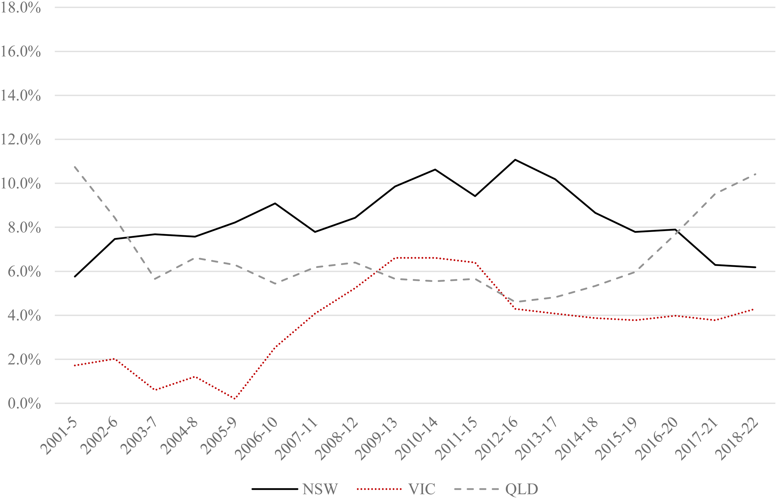
Random effects estimates of trends in the public–private sector wage gap in NSW, VIC and QLD 2001–2005 to 2018–2022.

Figure 6.

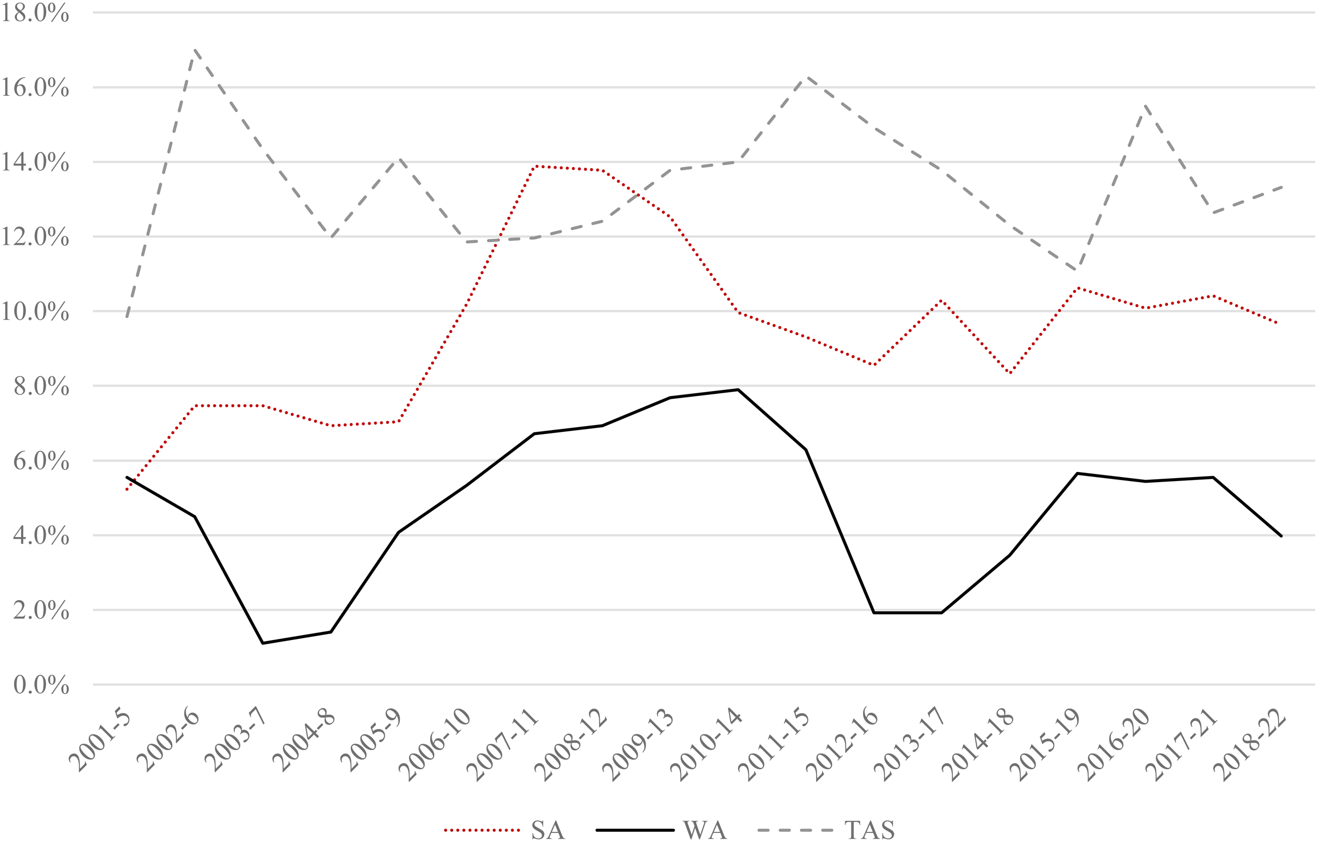
Random effects estimates of trends in the public–private sector wage gap in SA, WA, TAS 2001–2005 to 2018–2022.

As with the estimates at the national level, the public-sector gap also varies considerably over time within states. There is also little correlation in the trends between states. For example, the correlation coefficient associated with a comparison of NSW and VIC is equal to 0.50. A similar comparison of WA and QLD (two resource orientated states) reveals a correlation coefficient of 0.13. A comparison of NSW and TAS generates a correlation coefficient of 0.37.

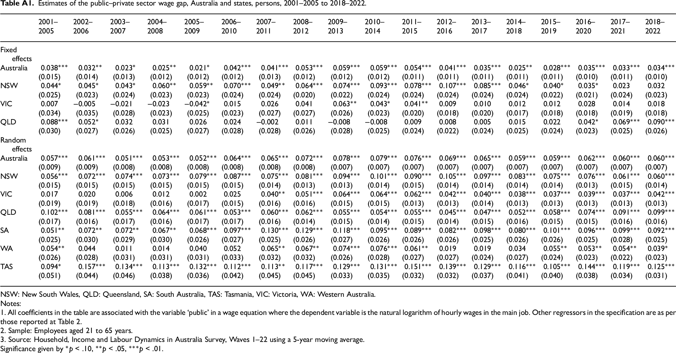
The FE results for NSW, VIC and QLD (Figure 4) show that when the public–private sector premium was increasing in NSW (over the early part of the 2000s) it was falling in VIC and QLD. Post the GFC there would appear to be catch-up in VIC. In recent years, the gap in QLD has been increasing while in the other states the pattern seems to be one of decline. The coefficient estimates associated with ‘Public’ in each of the FE regressions for the three states are provided in Table A1 in Appendix (the corresponding estimates for women are contained in Table S13 in the online supplemental appendix). In NSW the FE generated gap was statistically significant through to 2016–2020 and since then (2017–2021, 2018–2022) has not been significant. In VIC the gap was only significant in the 2009–2013 to 2011–2015 period. In QLD the gap was insignificant over much of the period examined and in recent years (2016–2020 to 2018–2022 has become statistically significant).

The RE estimates (also summarised in Table A1 in Appendix and Table S13 in the online supplemental appendix) show that, with the exception of WA, the gap has been statistically significant in all states since the GFC. In WA the gap was insignificant between 2012–2016 and 2014–2018. It may be that wage spill-over effects from strong growth in the resource sector served to minimise the public–private sector wage gap during these years. Indeed, Preston and Birch (2018) suggest that the mining boom was a key driver of stronger wage growth in WA relative to Australia. During 2018–2022 the WA public–private sector premium was marginally significant (10% level), whereas in all other states it was significant at the 1% level.

Trends in the public–private sector wage gap across the distribution

Finally, Figure 7 shows trends in the public–private sector wage gap across the distribution of persons. The estimates are generated using a FE quantile regression. The analysis considers the public–private sector wage gap for quantile 0.25 (low-paid workers) and quantile 0.75 (high-paid workers) as well as the mean and median of wages. We only focus on the outcomes nationally given the diversity of results at the state level.

Figure 7.

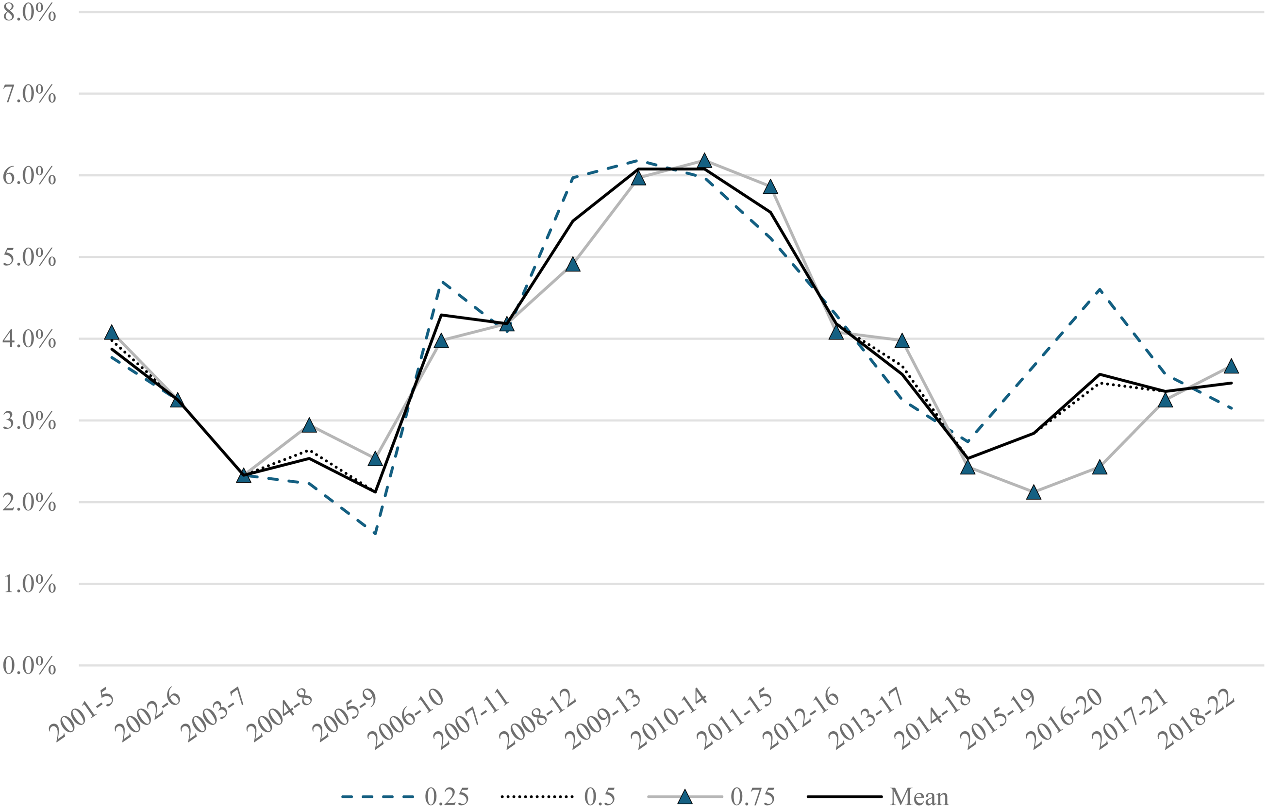
FE-Quantile estimates of trends in the public–private sector wage gap, Australia.

There are two distinct features in Figure 7. First, there are similar trends in the public–private sector earnings gap along the distribution over the period analysed up until 2014. Hence for most years, the gap is generally rising and falling in a similar manner for high-paid and low-paid workers. The main difference occurs in the 2014–2020 period when the premium is rising for low paid employees and falling for high-paid employees.

Second, differences in the earnings gap between high-paid and low-paid employees varies (without a consistent pattern). From 2003–2009 the public–private sector earnings gap was larger for high-paid workers than low-paid workers. This was also the case for 2010–2017. For other periods (such as 2017–2013 and 2013–2021), the public–private sector earnings premium was larger for low-paid workers.

Figure 8 presents the FE quantile regression results for women. The pattern is similar to that observed in Figure 7 (for persons), although a bit more accentuated. For example, in the GFC period the wage premium among low-paid public-sector women was falling at a faster rate than among high-paid public-sector women. From around 2013/2014, this trend reversed with the premium rising faster among low-paid public-sector women vis-à-vis their higher-paid counterparts. It may be that the public-sector wage caps had more of an impact on higher-paid workers and/or that government initiatives aimed at promoting women in the public sector benefited low-paid workers to a greater extent. It may also be that low-paid women in the private sector (e.g., in feminised areas such as childcare, retail trade and hospitality) experienced a faster slow-down in wage growth during this period, thus driving up the public-sector wage gap. Stewart et al. (2022), for example, show that wage growth in hospitality and retail trade has been slower than other industries since 2013. Relatedly, Martin (2024), suggests that childcare workers and retail workers are amongst the lowest paid workers in Australia.

Figure 8.

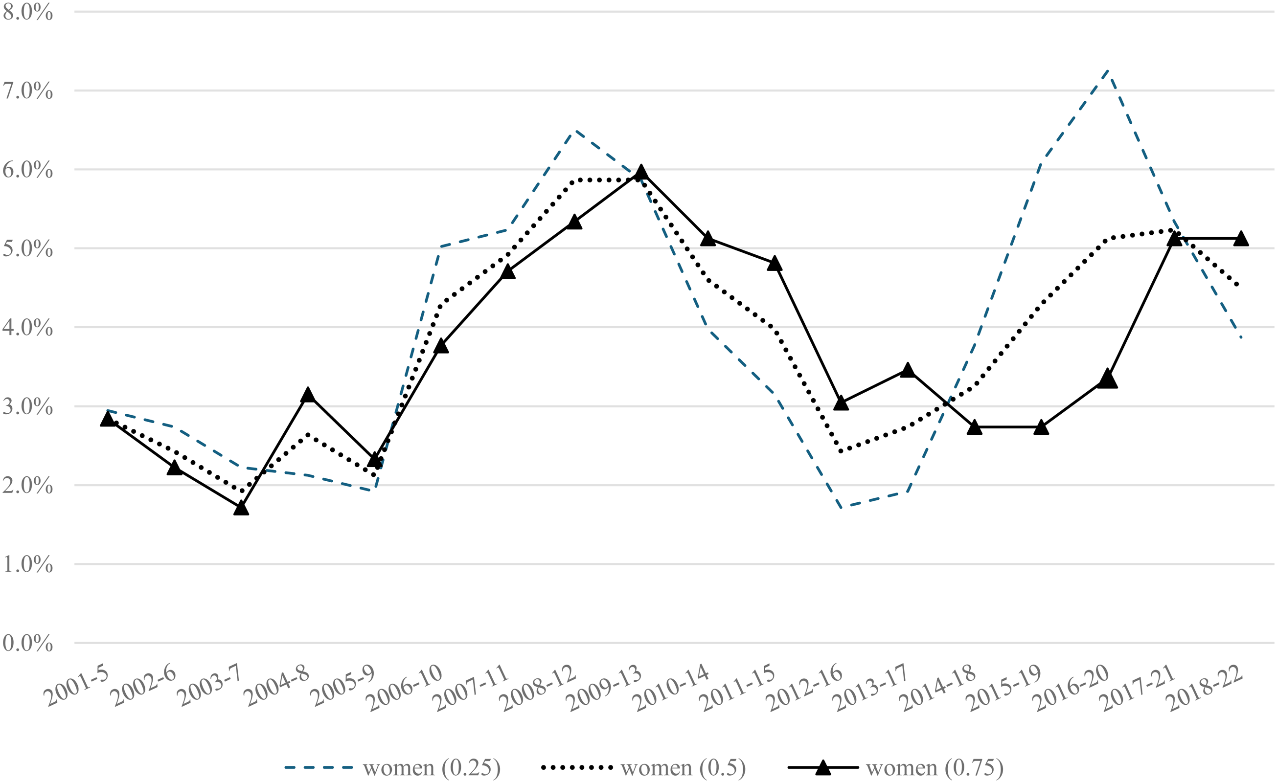
FE-Quantile estimates of trends in the public–private sector wage gap, Australia.

Summary and conclusion

This paper draws on data from the HILDA Survey to provide a detailed analysis of public–private sector wage gaps in Australia. To date Mahuteau et al. (2017) offer the most recent study of this wage differential in Australia, with their analysis also drawing on HILDA and covering the period 2001 to 2014. In the time since then the composition of the public sector has changed. For example, During 2001–2014, 42.8% of public-sector employees aged 21 to 65 were men, by 2015–22 this share had fallen to 39.6%. Similarly, during 2001–2014, 47.7% of public-sector employees held a degree, by 2015–22 this share had increased to 57.4%. Alongside these changes there has been a fall in real wage (Treasury, 2023) and the imposition of public-sector wage caps in some states. Accordingly, there are reasons to believe that the public-sector wage gap may have changed since the work of Mahuteau et al. and that a more recent analysis is warranted. The paper, therefore, has two main aims. The first is to extend the work of Mahuteau et al. by considering the gap in the 2015–2022 period. The second is to examine trends in the gap using 22 waves of data available in the HILDA Survey.

Our empirical work employs several approaches, including OLS and panel estimation techniques. For Australia as a whole and for the three large states (NSW, VIC and QLD) we primarily focus on the results generated using an FE panel estimator. In the smaller states (SA, WA and TAS) we rely on a RE estimator, noting that these results may suffer from endogeneity. Accordingly, no causality is claimed for the analysis concerning these states. We also disaggregate the results by persons, men and women.

Our main findings may be summarised as follows. First, in the period since 2014 the public-sector wage premium has increased for women and fallen for men. Indeed, in the case of men there is now no statistically significant gap at the national level. As at 2015–2022 the premium, at the mean, is 5.2% (significant at the 1% level) for women and 1.4% (statistically insignificant) for men. Second, the public-sector gap is now largely a female phenomenon; that is, it is driven by outcomes in the female labour market. Third, there is no obvious pattern in the magnitude of the public-sector premium across states. In VIC, for example, the wages of men and women in the public sector are qualitatively the same as those in the private sector. In NSW and QLD, in contrast, there is a highly statistically significant premium for women and an insignificant premium among men. Decomposition analysis also shows that the source of the gap (in terms of share of the raw public-sector wage gap that may be explained by differences in characteristics of public- and private-sector employees) differs across states.

Our fourth finding (based on a trend analysis using a 5-year moving window) shows that the public-sector premium is not constant over time and is neither procyclical, nor countercyclical. The fact that the trends differ by state lead us to our fifth finding: that public-sector wage gaps in Australia are more the product of local labour market forces rather than national pressures. Indeed, transition analysis using the panel aspect of HILDA shows that fewer than 10% of public-sector employees switch sectors (move to the private sector). This share is even smaller when considering those who move from the private to the public sector.

Our final finding, based on quantile analysis, is that the premium varies across the distribution, but not in a constant way by state or over time. Quantile analysis based on FE techniques shows that, post 2014, the premium among low-paid public-sector employees was above that of high-paid public-sector employees, although this pattern has reversed in recent times. It is possible that state sector wages policy such as wage caps have constrained the wages of higher paid public-sector employees to a greater extent than lower-paid public-sector employees, thus explaining the trends observed. Relatedly, it could be that interventions to improve gender equality in the public sector (WGEA, 2023) had a greater impact on the outcome of low-paid public-sector employees than higher-paid public-sector employees. A third explanation might be that real wages of low paid private-sector employees fell at a faster rate than low-paid public-sector employees.⁵

It is beyond the scope of this paper to explain why, nationally, the public–private sector wage premium has risen for women and fallen for men. We believe this should be a priority for future research. Further research might also fruitfully examine what is happening to public–private sector wage gaps by level of government employment. Within HILDA we are only able to identify whether an employee works in the public or private sector. Earlier work by Birch (2006) found that the gap was larger among federal government employees than it was among state government employees. Future work might also undertake a disaggregated analysis that incorporates the ACTs and the NT or investigate the gap within industries and occupations and/or examine why public- and private-sector employment is so ‘sticky’ (why is transition so small?).

Supplemental Material

sj-docx-1-jir-10.1177_00221856241300717 - Supplemental material for Public–private sector wage gaps in Australia: Extent, trends and gender

Supplemental material, sj-docx-1-jir-10.1177_00221856241300717 for Public–private sector wage gaps in Australia: Extent, trends and gender by Elisa Birch and Alison Preston in Journal of Industrial Relations

Footnotes

HILDA Disclaimer

This paper uses data from the Household, Income and Labour Dynamics in Australia (HILDA) Survey. We acknowledge that the HILDA Project was initiated and is funded by the Australian Government Department of Social Services (DSS) and is managed by the Melbourne Institute of Applied Economic and Social Research (Melbourne Institute). The findings and views reported, however, are those of the authors and should not be attributed to either the DSS or the Melbourne Institute.

Declaration of conflicting interests

The authors declared no potential conflicts of interest with respect to the research, authorship and/or publication of this article.

Funding

The authors received no financial support for the research, authorship and/or publication of this article.

ORCID iDs

Elisa Birch

Alison Preston

Supplemental material

Supplemental material for this article is available online.

Notes

Correction (January 2025):

The article has been updated with the addition of Disclaimer statement since its original publication. See correction notice for more details:

Author biographies

Elisa Birch is a senior lecturer in the Department of Economics at the University of Western Australia. Her research interests include labour economics and the economics of education.

Alison Preston is a professor of Economics at the University of Western Australia. Her research interests are in gendered aspects of employment, wage determination and financial literacy.

Appendix

Table A1.

Estimates of the public–private sector wage gap, Australia and states, persons, 2001–2005 to 2018–2022.

	2001–2005	2002–2006	2003–2007	2004–2008	2005–2009	2006–2010	2007–2011	2008–2012	2009–2013	2010–2014	2011–2015	2012–2016	2013–2017	2014–2018	2015–2019	2016–2020	2017–2021	2018–2022
Fixed effects
Australia	0.038***	0.032**	0.023*	0.025**	0.021*	0.042***	0.041***	0.053***	0.059***	0.059***	0.054***	0.041***	0.035***	0.025**	0.028***	0.035***	0.033***	0.034***
	(0.015)	(0.014)	(0.013)	(0.012)	(0.012)	(0.012)	(0.013)	(0.012)	(0.012)	(0.012)	(0.011)	(0.011)	(0.011)	(0.011)	(0.011)	(0.010)	(0.011)	(0.010)
NSW	0.044*	0.045*	0.043*	0.060**	0.059**	0.070***	0.049**	0.064***	0.074***	0.093***	0.078***	0.107***	0.085***	0.046*	0.040*	0.035*	0.023	0.032
	(0.025)	(0.023)	(0.024)	(0.023)	(0.023)	(0.024)	(0.024)	(0.020)	(0.022)	(0.024)	(0.024)	(0.024)	(0.024)	(0.024)	(0.022)	(0.021)	(0.024)	(0.023)
VIC	0.007	−0.005	−0.021	−0.023	−0.042*	0.015	0.026	0.041	0.063**	0.043*	0.041**	0.009	0.010	0.012	0.012	0.028	0.014	0.018
	(0.034)	(0.035)	(0.028)	(0.023)	(0.025)	(0.023)	(0.027)	(0.027)	(0.026)	(0.023)	(0.020)	(0.018)	(0.020)	(0.017)	(0.018)	(0.018)	(0.019)	(0.018)
QLD	0.088***	0.052*	0.032	0.031	0.026	0.024	−0.002	0.011	−0.008	−0.008	0.009	0.008	0.005	0.015	0.022	0.042*	0.069***	0.090***
	(0.030)	(0.027)	(0.026)	(0.025)	(0.027)	(0.028)	(0.028)	(0.026)	(0.028)	(0.025)	(0.024)	(0.022)	(0.024)	(0.025)	(0.024)	(0.023)	(0.025)	(0.026)
Random effects
Australia	0.057***	0.061***	0.051***	0.053***	0.052***	0.064***	0.065***	0.072***	0.078***	0.079***	0.076***	0.069***	0.065***	0.059***	0.059***	0.062***	0.060***	0.060***
	(0.009)	(0.009)	(0.008)	(0.008)	(0.008)	(0.008)	(0.008)	(0.008)	(0.007)	(0.007)	(0.007)	(0.007)	(0.007)	(0.007)	(0.007)	(0.007)	(0.007)	(0.007)
NSW	0.056***	0.072***	0.074***	0.073***	0.079***	0.087***	0.075***	0.081***	0.094***	0.101***	0.090***	0.105***	0.097***	0.083***	0.075***	0.076***	0.061***	0.060***
	(0.015)	(0.015)	(0.015)	(0.015)	(0.015)	(0.015)	(0.014)	(0.013)	(0.013)	(0.014)	(0.015)	(0.014)	(0.014)	(0.014)	(0.014)	(0.013)	(0.015)	(0.014)
VIC	0.017	0.020	0.006	0.012	0.002	0.025	0.040**	0.051***	0.064***	0.064***	0.062***	0.042***	0.040***	0.038***	0.037***	0.039***	0.037***	0.042***
	(0.019)	(0.019)	(0.018)	(0.016)	(0.017)	(0.015)	(0.016)	(0.016)	(0.015)	(0.015)	(0.013)	(0.013)	(0.014)	(0.013)	(0.013)	(0.013)	(0.013)	(0.013)
QLD	0.102***	0.081***	0.055***	0.064***	0.061***	0.053***	0.060***	0.062***	0.055***	0.054***	0.055***	0.045***	0.047***	0.052***	0.058***	0.074***	0.091***	0.099***
	(0.017)	(0.016)	(0.017)	(0.016)	(0.017)	(0.017)	(0.016)	(0.014)	(0.015)	(0.014)	(0.015)	(0.014)	(0.015)	(0.016)	(0.015)	(0.015)	(0.016)	(0.016)
SA	0.051**	0.072**	0.072**	0.067**	0.068***	0.097***	0.130***	0.129***	0.118***	0.095***	0.089***	0.082***	0.098***	0.080***	0.101***	0.096***	0.099***	0.092***
	(0.025)	(0.030)	(0.029)	(0.030)	(0.026)	(0.027)	(0.025)	(0.026)	(0.027)	(0.026)	(0.026)	(0.026)	(0.025)	(0.026)	(0.026)	(0.025)	(0.028)	(0.025)
WA	0.054**	0.044	0.011	0.014	0.040	0.052	0.065**	0.067**	0.074***	0.076***	0.061**	0.019	0.019	0.034	0.055**	0.053**	0.054**	0.039*
	(0.026)	(0.028)	(0.031)	(0.031)	(0.031)	(0.033)	(0.032)	(0.032)	(0.026)	(0.028)	(0.027)	(0.027)	(0.024)	(0.027)	(0.024)	(0.023)	(0.022)	(0.023)
TAS	0.094*	0.157***	0.134***	0.113***	0.132***	0.112***	0.113**	0.117***	0.129***	0.131***	0.151***	0.139***	0.129***	0.116***	0.105***	0.144***	0.119***	0.125***
	(0.051)	(0.044)	(0.046)	(0.038)	(0.036)	(0.042)	(0.045)	(0.045)	(0.033)	(0.035)	(0.032)	(0.032)	(0.037)	(0.041)	(0.040)	(0.038)	(0.034)	(0.031)

NSW: New South Wales, QLD: Queensland, SA: South Australia, TAS: Tasmania, VIC: Victoria, WA: Western Australia.

Notes:

1. All coefficients in the table are associated with the variable ‘public’ in a wage equation where the dependent variable is the natural logarithm of hourly wages in the main job. Other regressors in the specification are as per those reported at Table 2.

2. Sample: Employees aged 21 to 65 years.

3. Source: Household, Income and Labour Dynamics in Australia Survey, Waves 1–22 using a 5-year moving average.

Significance given by *p < .10, **p < .05, ***p < .01.

References

Abdallah

Coady

Jirasavetakul

(2023) Public-private wage differentials and interactions across countries and time. International Monetary Fund Working Paper WP/23/64, International Monetary Fund, Washington, United States. Available at: https://www.imf.org/en/Publications/WP/Issues/2023/03/17/Public-Private-Wage-Differentials-and-Interactions-Across-Countries-and-Time-531080

Belman

Heywood

(2004) Public wage differentials and the treatment of occupational differences. Journal of Policy Analysis and Management 23(1): 135–152.

Biesenbeek

van der Werff

(2019) Public private wage differentials: Evidence from The Netherlands. De Economist (Netherlands) 167(1): 23–43.

Birch

(2006) The public-private sector earnings gap in Australia: A quantile regression approach. Australian Journal of Labour Economics 9(2): 99–123.

Blackaby

Murphy

O’Leary

(1999) The payment of public sector workers in the UK: Reconciliation with north American findings. Economics Letters 65(2): 239–243.

Blackaby

Murphy

O’Leary

, et al. (2018) Regional pay? The public/private sector pay differential. Regional Studies 52(4): 477–489.

Blinder

(1973) Wage discrimination: Reduced form and structural estimates. Journal of Human Resources 8(4): 436–455.

Bonaccolto-Töpfer

Castagnetti

Prümer

(2022) Understanding the public-private sector wage gap in Germany: New evidence from a fixed effects quantile approach. Economic Modelling 116: 1–12.

Borland

Hirschberg

Lye

(1998) Earnings of public sector and private sector employees in Australia: Is there a difference? Economic Record 74(2224): 36–53.

10.

Cai

Liu

(2011) Public-Private sector wage gap in Australia: Variation along the distribution. British Journal of Industrial Relations 49(2): 362–390.

11.

Campos

Papapetrou

Depalo

, et al. (2017) Understanding the public sector pay gap. IZA Journal of Labor Policy 6(7): 1–29.

12.

Choi

Garen

(2021) The federal-private wage differential: How has it evolved? Applied Economics 53(5): 536–554.

13.

Clun

Crowe

(2022) You deserve more than thanks’: Albanese steps up pledge on pay. Sydney Morning Herald, 2 May. Available at: https://www.smh.com.au/politics/federal/you-deserve-more-than-thanks-albanese-steps-up-pledge-on-pay-20220502-p5aht4.html

14.

Colley

Woods

Head

(2022) Pandemic effects on public service employment in Australia. Economic and Labour Relations Review 33(1): 56–79.

15.

Dell’Aringa

Lucifora

Origo

(2007) Public sector pay and regional competitiveness. A first Look at regional public-private wage differentials in Italy. The Manchester School 75(4): 445–478.

16.

Giordano

Pereira

Depalo

, et al. (2015) The public sector pay gap in a selection of euro area countries in the pre-crisis period. Review of Public Economics 214(3): 11–34.

17.

Halvorsen

Palmquist

(1980) The interpretation of dummy variables in semilogarithmic equations. American Economic Review 30(3): 474–475.

18.

Hastie

(2023) Cook goes back to basics for New WA public sector pay policy. WA Today, 8 December. Available at: https://www.watoday.com.au/politics/western-australia/cook-goes-back-to-basics-for-new-wa-public-sector-pay-policy-20231218-p5es7h.html

19.

Jean

Groves

(2024) Workplace gender equality agency scorecard shows women in the public service are paid 13.5pc less than men, but the gaps is even bigger in the private sector. ABC News, 20 June. Available at: https://www.abc.net.au/news/2024-06-20/women-earn-less-than-men-in-public-and-private-sector/103995276

20.

Jones

(1983) Sources of gender inequality in income: What the Australian census says. Social Forces 62(1): 134–153.

21.

Kehoe

(2020) K-shaped’ recession as public service swells. The Australian Financial Review, 9 September. Available at: https://www.afr.com/policy/economy/k-shaped-recession-as-public-service-swells-20200908-p55tk6

22.

Mahuteau

Mavromaras

Richardson

, et al. (2017) Public-Private sector wage differentials in Australia. Economic Record 93(S1): 105–121.

23.

Makridis

(2021) (Why) is there a public/private pay gap? Journal of Government and Economics 1: 1–9.

24.

Marin-Guzman

(2023) ‘The wage cap is dead’: NSW public servants accept 4pc pay rise. Australian Financial Review, 21 July. Available at: https://www.afr.com/work-and-careers/workplace/the-wage-cap-is-dead-nsw-public-servants-accept-4pc-pay-rise-20230721-p5dq6n

25.

Martin

(2024) Why are child carers still paid less than retail workers? and how can we help fix it? The Conversation, 13 August. Available at: https://theconversation.com/why-are-child-carers-still-paid-less-than-retail-workers-and-how-can-we-help-fix-it-236563

26.

Michael

Christofides

(2020) The impact of austerity measures on the public-private wage gap in Europe. Labour Economics 63: 1–20.

27.

Murphy

Blackaby

O’Leary

, et al. (2020) Understanding what has been happening to the public-sector pay premium in Great Britain: A distributional approach based on the labour force survey. British Journal of Industrial Relations 58(2): 737–300.

28.

Nowak

Preston

(2001) Can human capital theory explain why nurses are so poorly paid? Australian Economic Papers 40(2): 232–245.

29.

Oaxaca

(1973) Male-Female wage differentials in urban labor markets. International Economic Review 14(3): 693–709.

30.

Office for Women (2024) Queensland women's strategy 2016-21. Available at: https://www.women.qld.gov.au/about-us/about-office-for-women (accessed 22 November 2024).

31.

Office of the Special Commissioner, Equity and Diversity (2023) Queensland public sector gender pay equity dashboard 2023. Available at: https://www.psc.qld.gov.au/_publications/Queensland-public-sector-Gender-pay-equity-dashboard-2023.pdf (accessed 22 November 2024).

32.

Preston

(2001) The Structure and Determinants of Wage Relativities: Evidence from Australia. Surrey, United Kingdom: Ashgate Publishing.

33.

Preston

Birch

(2018) The western Australian wage structure and gender wage gap: A post mining boom analysis. Journal of Industrial Relations 60(5): 619–646.

34.

Rattsø

Stokke

(2019) Identification of the private-public wage gap. Labour Economics 59: 153–163.

35.

Risse

(2023) Unseen and undervalued: how much is ‘women’s work’ undervalued in the economy? Opinion Article, Committee for Economic Development of Australia (CEDA), Canberra, Australia. Available at: https://www.ceda.com.au/newsandresources/opinion/workforce-skills/unseen-and-undervalued-how-much-is-womens-work (accessed 22 November 2024).

36.

Stewart

Stanford

Hardy

(2022) The wages crisis: Revisited. The Australian Institute, Canberra, Australia. Available at: https://australiainstitute.org.au/wp-content/uploads/2022/05/Wages-Crisis-Revisited-WEB.pdf (accessed 22 November 2024).

37.

Treasury (2023) Working future, the Australian government’s white paper on jobs and opportunities. Australian Treasury, Canberra, Australia. Available at: https://treasury.gov.au/employment-whitepaper/final-report (accessed 22 November 2024).

38.

Workplace Gender Equality Agency (2023) 2022 commonwealth public sector gender equality snapshot. Workplace Gender Equity Agency, Sydney Australia. Available at: https://www.wgea.gov.au/publications/public-sector-snapshot-2022 (accessed 22 November 2024).

Supplementary Material

Please find the following supplemental material available below.

For Open Access articles published under a Creative Commons License, all supplemental material carries the same license as the article it is associated with.

For non-Open Access articles published, all supplemental material carries a non-exclusive license, and permission requests for re-use of supplemental material or any part of supplemental material shall be sent directly to the copyright owner as specified in the copyright notice associated with the article.

0.00 MB

0.16 MB

Public–private sector wage gaps in Australia: Extent,trends and gender

Abstract

Keywords

Introduction

Approach

Dummy variable approach

Blinder-Oaxaca decomposition approach

Panel estimators

Quantile approach

Time period

Data, variables, sample and descriptive statistics

Data and variables

Sample

Descriptive statistics

Results

The public–private sector wage gap at the mean—using the dummy variable approach

State public–private sector wage gaps at the mean—dummy variable approach

Blinder-Oaxaca decomposition—what's driving the sector-wage gaps?

National and state public–private sector wage gaps across the wage distribution

Robustness checks

Without occupation

Trends in the public–private sector wage gap—nationally and by state

Trends in the public–private sector wage gap across the distribution

Summary and conclusion

Supplemental Material

sj-docx-1-jir-10.1177_00221856241300717 - Supplemental material for Public–private sector wage gaps in Australia: Extent, trends and gender

Footnotes

HILDA Disclaimer

Declaration of conflicting interests

Funding

ORCID iDs

Supplemental material

Notes

Correction (January 2025):

Author biographies

Appendix

References

Supplementary Material