Predicting the fiber orientation of injection molded components and the geometry influence with neural networks

Abstract

The injection molding simulation of short fiber reinforced plastics (SFRP) is time consuming. However, until now it is necessary for predicting the local fiber orientation, to optimize the molding process and to predict the mechanical behavior of the material. This research presents the capabilities of artificial neural networks (NN) in predicting fiber orientation tensor (FOT) during injection molding processes, with a focus on enhancing computational efficiency compared to traditional simulation methods. Three NN architectures are compared based on simulated injection molded plates, with the goal of predicting the effect of the plate geometry on the local fiber orientation. Results indicate that NN outperform the baseline assumption of aligned fibers and demonstrate significant potential for accurate FOT prediction. The computational efficiency of NN, especially during the prediction phase, showcases a reduction in processing time by a factor of 10⁴ compared to traditional simulation methods. This research lays a foundation for further exploration into the feasibility of NN in partly replacing time-consuming simulations for practical applications in injection molding processes.

Introduction

The usage of SFRP in many industry sectors is well established and the prediction of its behavior is critical for a major part of all supply and construction chains.^1,2 Due to their substructure which is dominated by the fiber orientation SFRP performs strongly anisotropic. ³ This dependency must be considered for accurate predictions of the behavior of components made from SFRP.^4,5 Therefore, in the last decades much effort was invested to establish precise models of the fluid dynamics of viscous materials and the interaction of fibers carried along. This has resulted in molding simulations based on methods and models with a high confidence-level capable of predicting the critical dependencies reliably.^6–12

Still the availability of predictions of the local fiber orientations is often a bottle neck because such molding simulations are time consuming and have a high cost in computational power. This applies in particular to mobility applications with high security requirements, because during the developing and designing phase the demands for rapid iterations are usually too high to wait for a molding simulation. This is especially true, as a change in the component shape results in completely different local FOTs because the fiber distribution is mainly determined by the geometry of the molded part.

Thus, there is a great need for a FOT prediction with a maximal computing time of several minutes, even for complex geometries. Such predictions wouldn’t have to be perfectly precise, as for a final evaluation after the designing iterations a larger time investment with the detailed molding simulation can be justified.

The recent prominent developments in the field of AI create a spotlight on this method of analyzing and forecasting data and its applications in engineering. ¹³ NN in particular have shown a great capability to learn complex dependencies in data without much human intervention needed. ¹⁴

A rule of thumb is, that AI is typically successful if a large data basis is available with the output data showing strong correlation to the input data.^15,16 With the currently available computed tomography (CT) scan technologies it is impossible to create such a large data basis within manageable expenses. Therefore, this study is based on data produced by simulations, with a previously fitted and validated simulation model. To have good correlations in the data an appropriate set of geometries was chosen, while keeping it as simple as possible (see chapter 3).

Alongside natural speech processing and generation AI was very successful in two areas, which are applicable for the molding of SFRP. Firstly, AI is an effective tool for image recognition and generation, which is a 2D application but was also transferred to 3D shape recognition (for example PointNet ¹⁷ ). This aligns well to predicting FOTs, as the NN needs to recognize the shape of the component geometry and connect it to the influence on the local fiber distribution. Secondly, the successes in forecasting of time series for example for weather forecasts or stock markets^18–20 could be transferred to the prediction of flow patterns of SFRP with one special dimension interpreted as time dimension. Therefore, these two concepts will be tested in the following.

The goal of this paper is to give a first insight on whether it is possible to predict local FOTs with NN and to determine which architectures achieve the best results, as the research on this application of AI is sparse. Because large experimental data on FOTs in injection molding can only be obtained with extremely high effort, the presented method is based on simulated data exclusively while using a verified simulation model. Therefore, in the foreseeable future the NN applied to injection molding will always rely on traditional injection molding simulations. The aim is not to outperform molding simulations in accuracy but to significantly speed up the process. The method of using NN would then perfectly complement the traditional approach for all applications requiring a “quick first prediction”.

Methods & material

Short fiber reinforced plastics (SFRPs)

Short Fiber Reinforced Plastics (SFRPs) describe a type of material that combines a matrix material with a reinforcing fiber material. The matrix, here consisting of polypropylene (PP), maintains the shape and form of the component and provides great manufacturing flexibility and a high capability to absorb energy. The reinforcing fibers, in this case made of glass, significantly influence the mechanical properties of the composite material. They primarily enhance strength and stiffness. This leads to materials characterized by high strength-to-weight ratios, excellent fatigue resistance, and extensive design flexibility. The properties of SFRPs do not only depend on characteristics of the matrix and the fibers but also the orientation of the fibers play a significant role.

This study is focused on the injection molding manufacturing process. In this process, the fibers mixed with a thermoplastic polymer, are heated, and then injected under pressure into some dice. In the viscous liquid the comparably short fiber, in our case 1-2 mm, are subjected to many forces influencing their orientation. The fiber orientation is mainly determined by the geometry of the molded part. Notably, in this study the focus is therefore on the geometry influence, and neither on the influence of process parameters nor on different materials.

In a straight plate typically three layers are formed in thickness direction with fiber pointing in the molding direction due to friction with the dice and 90° rotated fibers in the middle. The orientation changes if the plate is bent. At holes and edges fiber accumulate. Behind holes weld lines are formed. Moreover, depending on the component, a multitude of additional effects can.

Although in theory the FOT in large components could be scanned by CT, this is too much effort and in practice simulations are performed and verified instead. Likewise in this research all data is generated by simulations with a verified material model from literature.

Molding simulations

Fiber orientation predictions play an important role in understanding the behavior of fiber-reinforced composites, as the composite performance is greatly influenced by the local fiber orientation. Their modelling by correct simulations is important as it allows manufacturers to assess the potential strength, stiffness and overall performance before the final product is manufactured. One of the most frequently used models is the Folgar-Tucker model. ²¹ It describes the development of the second-order fiber orientation tensor and considers several factors such as the viscosity of the matrix, the ratio of fiber diameter to length and the flow velocity field. An important aspect of the Folgar-Tucker model is the choice of closure, i.e. the mathematical closure used to describe the fiber orientation distribution. Examples of closures that are widely used are quadratic, linear, and orthotropic. For detailed overview of closure approximations, we refer to Al-Qudsi et al. ²² In the current work a smooth orthotropic closure approximation is applied.

The injection simulations are performed with FLUID, ²³ a simulation tool developed in Fraunhofer Institute for Industrial Mathematics (Fraunhofer ITWM), department of Flow and Material Simulations. It was conceived and developed to perform simulations of non-Newtonian systems ranging from single-phase shear-thinning fluids to multiphase suspensions such as flow of reinforced concrete. ²⁴ One of FLUID’s capabilities is the simulation of injection molding processes. These involve solving equations to predict and analyze the behavior of the molten plastic suspension in a mold during the injection molding process. The Navier-Stokes equations build the fundament, as they describe the velocity and pressure fields. These equations are supplemented by the energy conservation equation, that accounts for the temperature distribution in the mold. Equations for fiber orientation, used to predict the orientation of the fibers in the suspension, complete the overall system.^25,26

A non-Newtonian, shear-thinning liquid was used as simulation model. The density of the matrix material was set to 1139 (kg/m³) and the viscosity was modelled using the well-known Carreau model (see Figure 1). For simplicity, isothermal flow conditions were assumed. The fiber orientation is modelled by the Folgar-Tucker equation with a diffusion coefficient of 0.0035, a fiber length of 10 mm and a diameter of 0.01 mm. The model was optimized and validated on CT scans and simulations of plates and more complex components in a public project from 2020. ²⁷

Figure 1.

The applied Carreau viscosity with respect to the shear rate.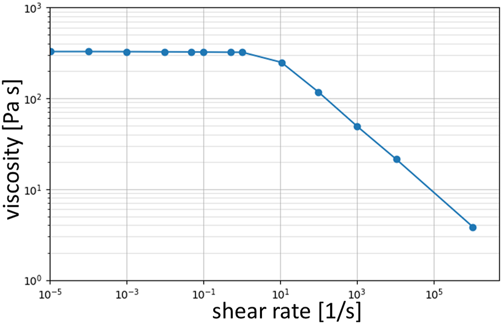

Neural network architectures

To evaluate the potential capability of NN in predicting the local FOT, three different architectures were investigated. The aim here was not to develop a new AI method, but to apply established methods to a new field and to discover the most promising approach. As the molding simulation is performed on a mesh grid of finite elements the data is previously organized on a regular mesh grid with constant shape (see chapter 3).

Dense Neural Networks (DNN) constitute the foundational architecture explored in this study. DNNs consist of layers of interconnected nodes, where information flows unidirectionally from input to output. Thereby between neighboring layers all nodes are fully connected as shown in Figure 2. Here the input mesh grid is first flattened to a single 1D input vector. The model learns from the input data, adjusting weights and biases to minimize the error in predicting the desired output. DNNs provide a straightforward approach and are not based on prior knowledge about the data. For the data in this research an architecture with 10 layers and 100 neurons per layer showed the best performance resulting in about 22 million trainable parameters.

Figure 2.

The architecture of a DNN with input layer, hidden layers and output layers fully connected.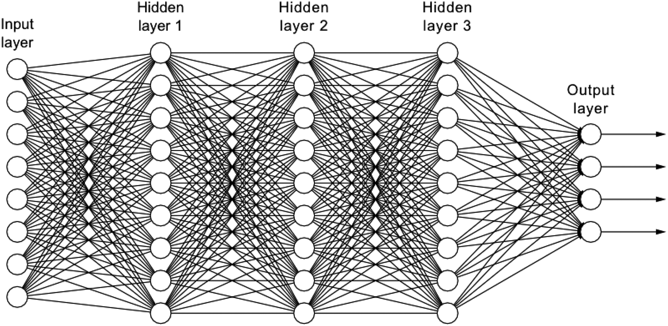

Convolutional Neural Networks (CNNs) are well-suited for spatial data ²⁸ like the fiber orientation patterns in SFRPs and typically significantly outperforming DNNs on more dimensional spatial input data. This network architecture is often utilized for 2D and 3D image recognition. A common CNNs consist of a convolutional layer, extracting local features from input data, and a pooling layer, reducing the spatial dimensionality to keep the model computationally efficient (see Figure 3). The convolutional layer involves sliding kernels over the input grid, performing element-wise multiplications and summations to extract features generating the so-called feature map. The subsequent pooling layer divides this feature map into nonoverlapping parts only keeping the most relevant information of each region, for example the maximum value. The pooling operation can be applied to three dimensions analogously to the convolution operation. The best performance could here be achieved with a kernel size = 4, three convolutional layers with 64, 128 and 256 features respectively, followed by a dense layer of 512 and the output layer. Overall, this entails 130 million trainable parameters.

Figure 3.

The outline of a CNN with input, the padding, the multiplication with the kernel, the resulting feature map, and the pooling.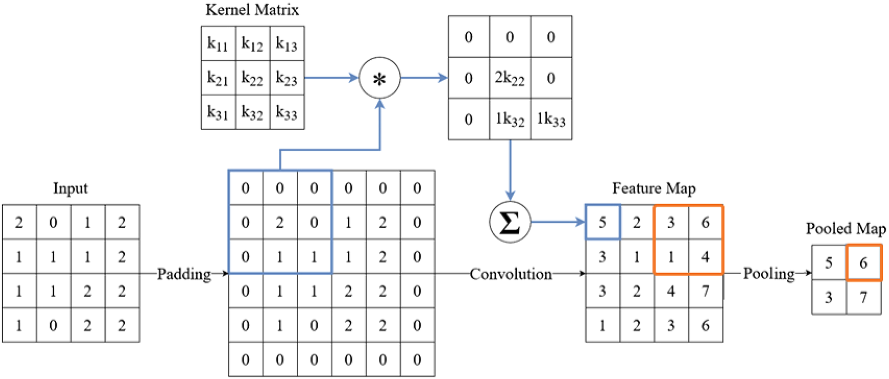

The final architecture considered for the prediction task is a Recurrent Neural Network (RNN) often used for predicting time series. Unlike the previously explored architectures, which classify as Feed Forward Neural Networks (FFNNs), a RNN introduces a memory component to the model that allows predictions to be influenced not only by the current input, but also by the network’s previous states (see Figure 4). This characteristic aligns well with the underlying concept of the injection molding process. The RNN might be able to model the gradual evolution of fiber orientations as the mold gets filled from left to right. Unlike abrupt changes, the FOTs are expected to change rather gradually across the spatial coordinates, with the filling direction assumed as the most important factor. Consequently, the third spatial direction (the filling direction) is interpreted as the time dimension. For this purpose, the input mesh grid is separated into 2D slices and fed to the RNN sequentially.

Figure 4.

The outline of a RNN with sequence input, an iterative prediction, and the hidden state.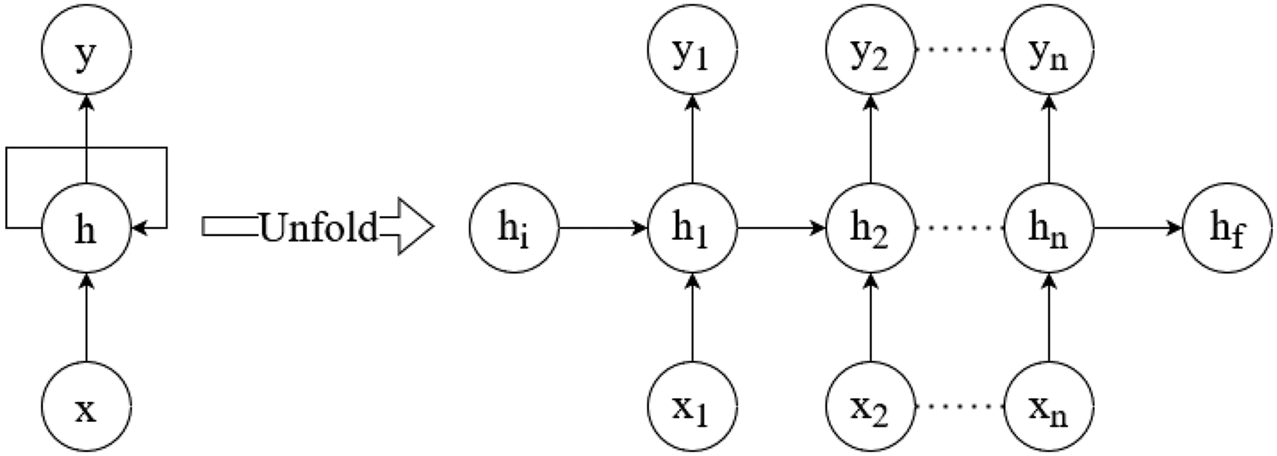

Recurrent Neural Network (RNN) in general have the problem of losing information over longer time iterations and of vanishing gradients for the parameter optimization. ²⁹ Thus in this research an enhanced RNN network is employed: the so-called Long Short Term Memory (LSTM) network first introduced by Hochreiter and Schmidhuber. ³⁰ The LSTM has a more elaborate method of keeping the relevant information in the memory state due to special input, forget and output gates (see Figure 5). As the spatial characteristic of the features remain as two-dimensional grids of the original 3D mesh, a network with a ConvLSTM2D layer was employed, combining the benefits of both the LSTM network and the previously used convolutional network. While this network type is a hybrid of a convolutional and a recurrent model, it will be continuously referred to as LSTM, to maintain clarity when comparing the different models. Here only two recurrent layers were necessary to achieve the best performance with each 25 features followed by dense output layer. Therefore, only 20 million free parameters were trained.

Figure 5.

A schematic overview of a LSTM with the iterative input and output, the forget gate, the input gate, and the output gate.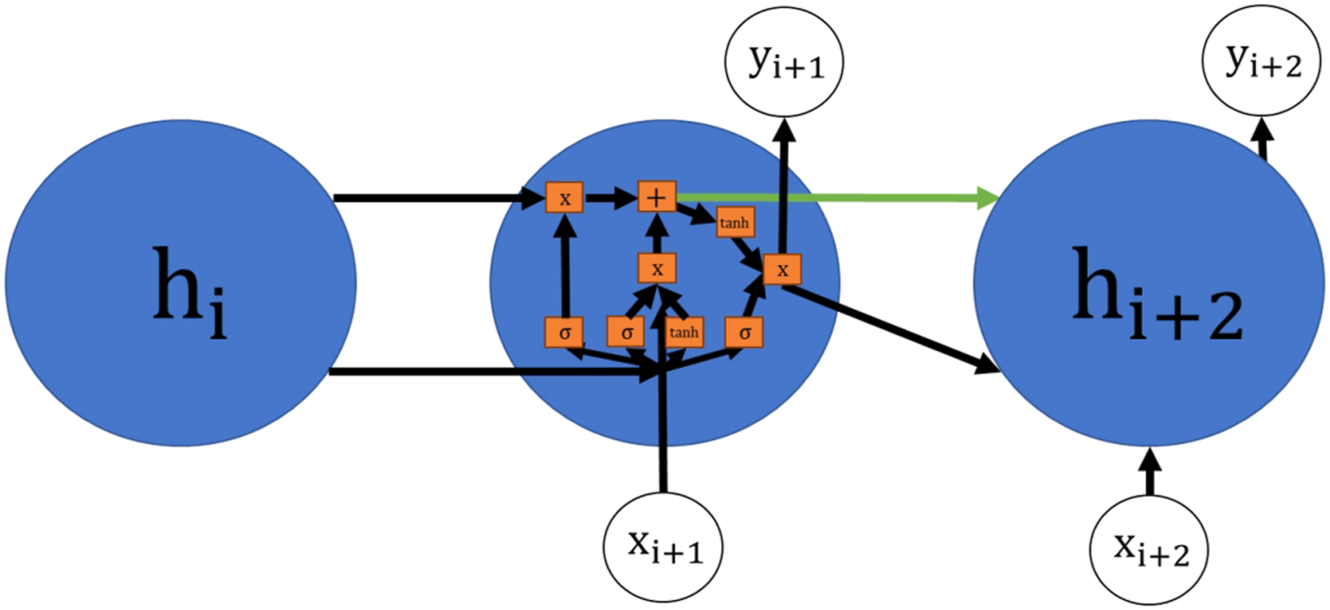

Transformer architecture have recently gained a lot of attention with the great success of Large Language Models (LLM), still in this research they were not tested. The key elements of transformer architectures are an embedding of all possible input subsequences as well as an attention mechanism. ³¹ Accordingly, the models have great generalizing capabilities and context knowledge, but they have a need for a very large data basis, hence the name “Large” Language Models. As such a large data basis is not available for molding simulations transformer architecture were not easily applicable here.

A NN is typically characterized by two parameter sets, the trainable parameters and the hyperparameters. The trainable parameters, which are present inside the network, for example in the form of weights and biases, are the elements that enable the learning of a NN. As a model gets trained by minimizing an error function for some training data, these parameters get adapted, to let the model make more accurate predictions. The hyperparameters, on the other hand, include the external configurations of a model and are chosen prior to the training process.

For this study, the Rectified Linear Unit (ReLU) was used as activation function for all layers (except the output layer, where a sigmoid function was used). ReLU was chosen due to its computationally efficient introduction of the needed non-linearity to let the model capture complex patterns while yielding generally good performances on a variety of tasks ³² (see Figure 6). For the learning process, the ADAM optimizer ³³ was employed to update the weights and biases of the models. It works by calculating the first and second momentum for the gradient descent operation, the commonly used optimization algorithm and adapts the learning rate based on these moments, making it a versatile and popular choice as an optimizer.

Figure 6.

A depiction of the ReLU activation function.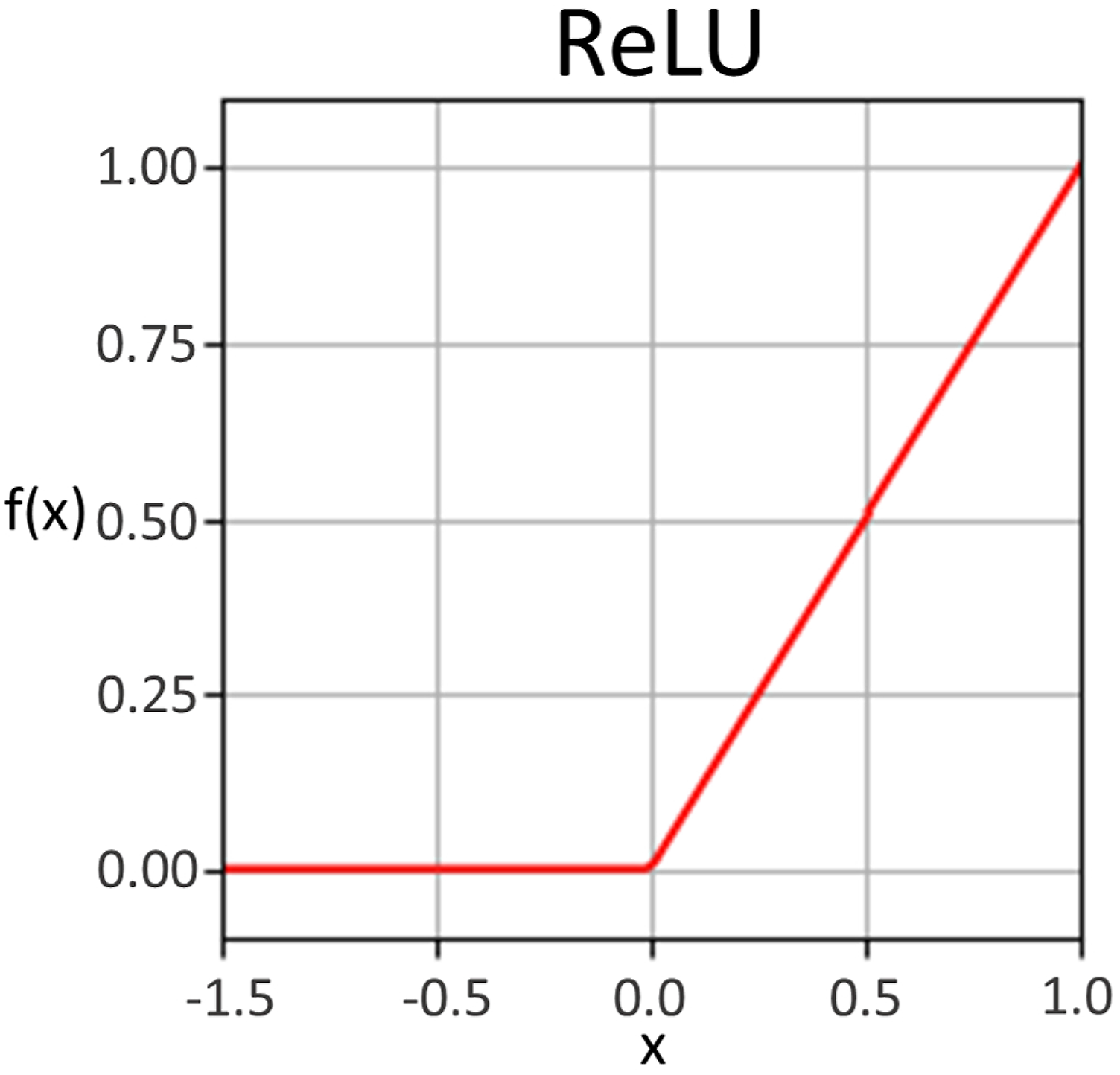

Other parameters, which include the number of training epochs, the batch size, the concretely employed architecture, like the depth and the widths of the models, as well as the number of kernels for convolutions, the amount of LSTM layers and special techniques like dropout, to prevent overfitting, were manually varied and adapted for the different models.

This study was conducted using the machine learning framework TensorFlow together with Keras, the high-level NN library for the programming language Python and with the Python extension NumPy used for data preparation and postprocessing. An exception to this is of cause the molding simulation, which was performed in FLUID, as mentioned above.

Data basis

Providing real experimental data of the local fiber orientation from molded components can in principle be done by CT scans. However, this is costly and time-consuming and therefore normally only performed on small volumes to have a sufficiently high resolution. Thus, this research relies on the simulation of the molding process with a simulation model that was previously validated on CT scans as explained above. ³⁴

The injection molding process with SFRP was simulated for 200 plates, each defined by a unique set of geometry parameters. The plate geometries are a cuboid with a fixed width of 50 mm in the x direction, a variable length of 60 mm to 90 mm in the y direction, and a variable thickness of 2 mm to 3.5 mm in the z direction. It was ensured that the plate had at least 7 elements in the thickness direction during the simulation. Additionally, each plate had a circular cut-out, characterized by the x and y coordinates of the center and the radius of the hole, as shown in Figure 7.

Figure 7.

A depiction of one of the plate geometries with a varying plate length, plate thickness, hole radius and hole coordinates.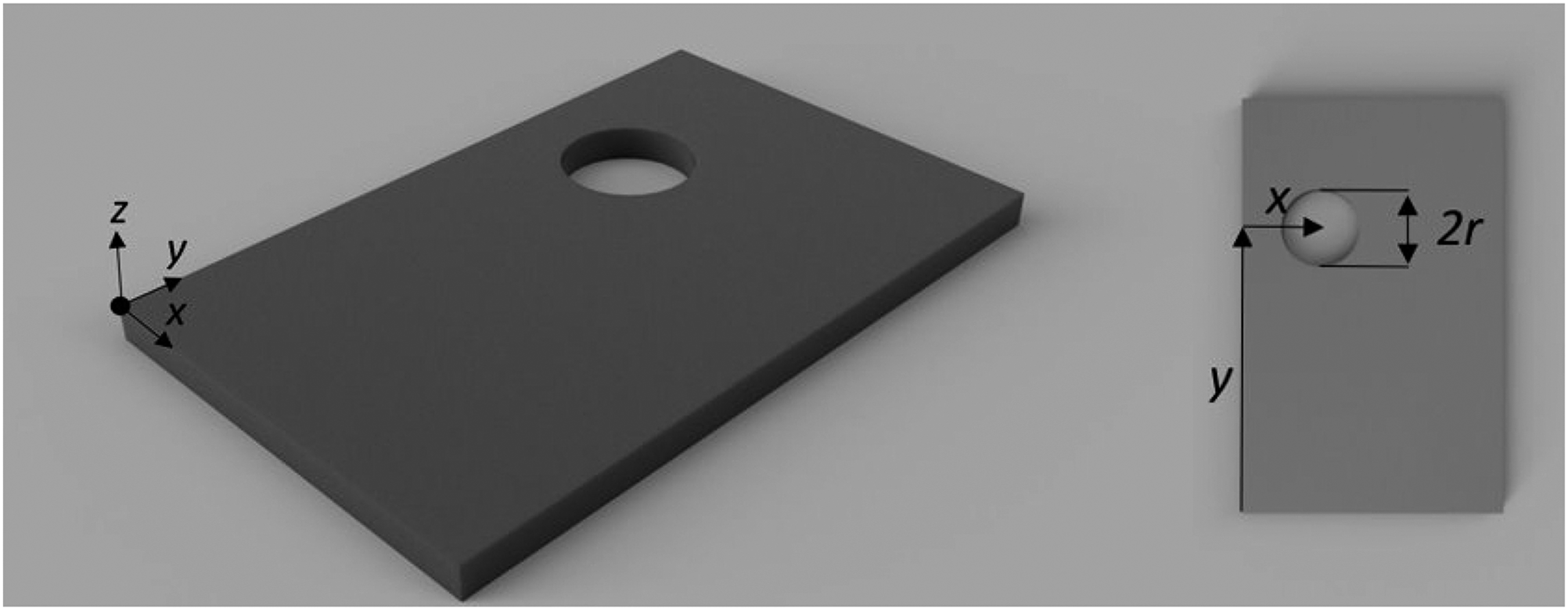

The filler neck for the molding process was located parallel to the x axis, resulting in an injection flow in the y direction. This geometry was chosen for its simplicity ensuring a problem-free data generation phase as well as reasonable small input and output matrices. Despite this simplicity, it introduces sufficient complexity for the molding process in particular with the presence of the cut-out to differentiate the resulting FOT distributions for distinct geometries, as illustrated in Figure 8.

Figure 8.

Four examples of the results in plates of varying length using traditional molding simulations with the software FLUID. Color coded is the percentage of fibers in × direction.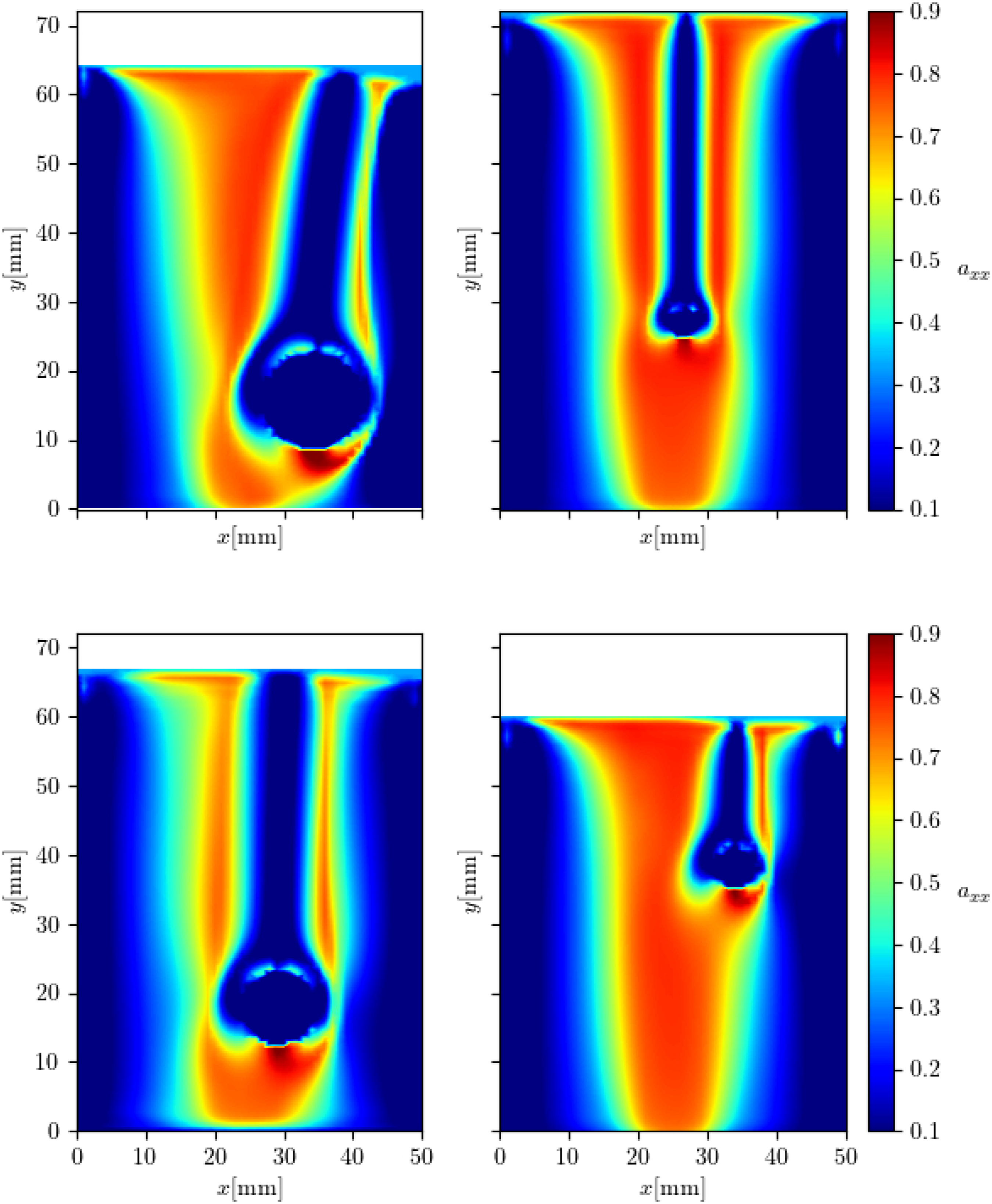

In Figure 8 a top-down view of the mid most elements in thickness direction (z) is shown. Color-coded is the A_xx element of the FOT corresponding to the percentage of fibers in x direction. The influence of the left and right dice wall is strongly visible leading to less than 15% of fibers in x-direction near the left and right edges. Also, fibers are accumulating at the end of the plate and aligning with the dice wall in x-direction. An even stronger but very local accumulation can be seen in front of the holes. The fluid flows around the hole and forms a weld line behind it with unoriented fibers (forming the blue tail) that continues until the end of the plate.

Overall, this data and the chosen component geometry are suitable as a starting point for analyzing the capability of NN to predict local FOTs.

After the simulation of all plates the local FOTs were mapped on a regular grid with 51 × 101 × 7 elements paying no heed to the geometry parameters. This makes a simple handling of the data possible for the NN. Altogether, the output data consisted of 200*51*101*7*6 = 43 268 400 values (plate number * x-dim * y-dim * z-dim * FOT elements).

The input for each plate was also organized on a mesh grid with the same dimensions. The information on the grid points could be chosen in different ways. One could either give the local x-, y-, z- coordinate and indicating the hole with a negative sign. Or one could give a binary input with 1 for points in plate and 0 for points in the hole while additionally supplying the NN with the grid spacing as metadata. In this study features were applied that are specialized for the tested geometries. The features consisted of the local x-, y- coordinate minus the x-, y- coordinate of the hole. By doing this, the most important information is handed to the network, even capturing the information, if the point is behind or in front of the hole. However, additional testing indicates that all input features are viable. These results will not be show here in detail, as this paper is intended as an overview on the performance of different model architecture.

Before training the models, the input and output data were prepared to be better suited as training data for a NN model. This involves centering around zero and normalizing the range to achieve better training results without falsely favoring the features of lager scales. ³⁵

A commonly encountered problem, when training NN, is overfitting. This refers to a model being too well adapted to the training data, rather memorizing the data itself, than capturing patterns from it, resulting in very good performance on the data it has been trained on, while making bad predictions for data not seen during optimization. To avoid this, the data was split into three disjoint sets:

• Training set – data on which the network is trained and optimized.

• Validation set – data on which the network can verify its generalization progress being excluded by the training itself. The performance check is used to optimize hyperparameters.

• Test set – data the network will not see during optimization of the model and its architecture to test the final trained model on an unseen dataset.

As the amount of data for this study was limited, the test and the validation sets were kept small, with each set containing 15 simulated plates, while the training data included the remaining 170.

Results

After creating the data basis with the molding simulations and preparing the data for ease of training, the three architectures to be tested where implemented. They were trained on the data and their hyperparameters were optimized. Afterwards, their capability of predicting the local FOTs can be judged by calculating the mean square error (MSE) between the predicted and the simulated FOT data. Additionally, the models were compared to a random fiber orientation and a baseline assuming all fibers aligned in molding direction (see Figure 9). For each NN model, the corresponding MSE values for the training and validation sets are illustrated.

Figure 9.

The performance of the three tested architecture measured by MSE compared with a random orientation and the baseline.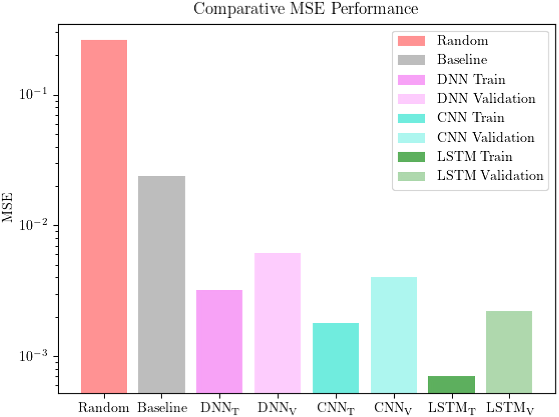

All the architectures outperform the baseline significantly. The increased complexity of the CNN and the LSTM architecture seem to enhance their prediction capabilities over the simpler DNN. The LSTM network achieved the best results of the three networks, with an MSE of 7 × 10−4 on the training data and 2.5 × 10−3 on the validation data. This recurrent model therefore predicts the FOTs from unseen feature sets almost as accurately as the best CNN could predict for data it has seen during optimization. Despite this superb performance, it is worth mentioning that the training process of the LSTM network was far more computationally expensive taking 23h while the CNN is trained within 5 min and the DNN within 1 min.

Once a trained model is available, the prediction process for hundreds of plates is a matter of seconds for all discussed architectures. This presents a strong contrast to the molding simulations, which require multiple hours for simulating a single plate and thus are dramatically outperformed by the NN. The predictions exhibit an impressive boost in speed, exceeding factors of 10,000 for the time needed to predict the FOTs for a single plate. All these calculation times were achieved on a single machine with 4 cores and could even be improved by moving to a computing cluster.

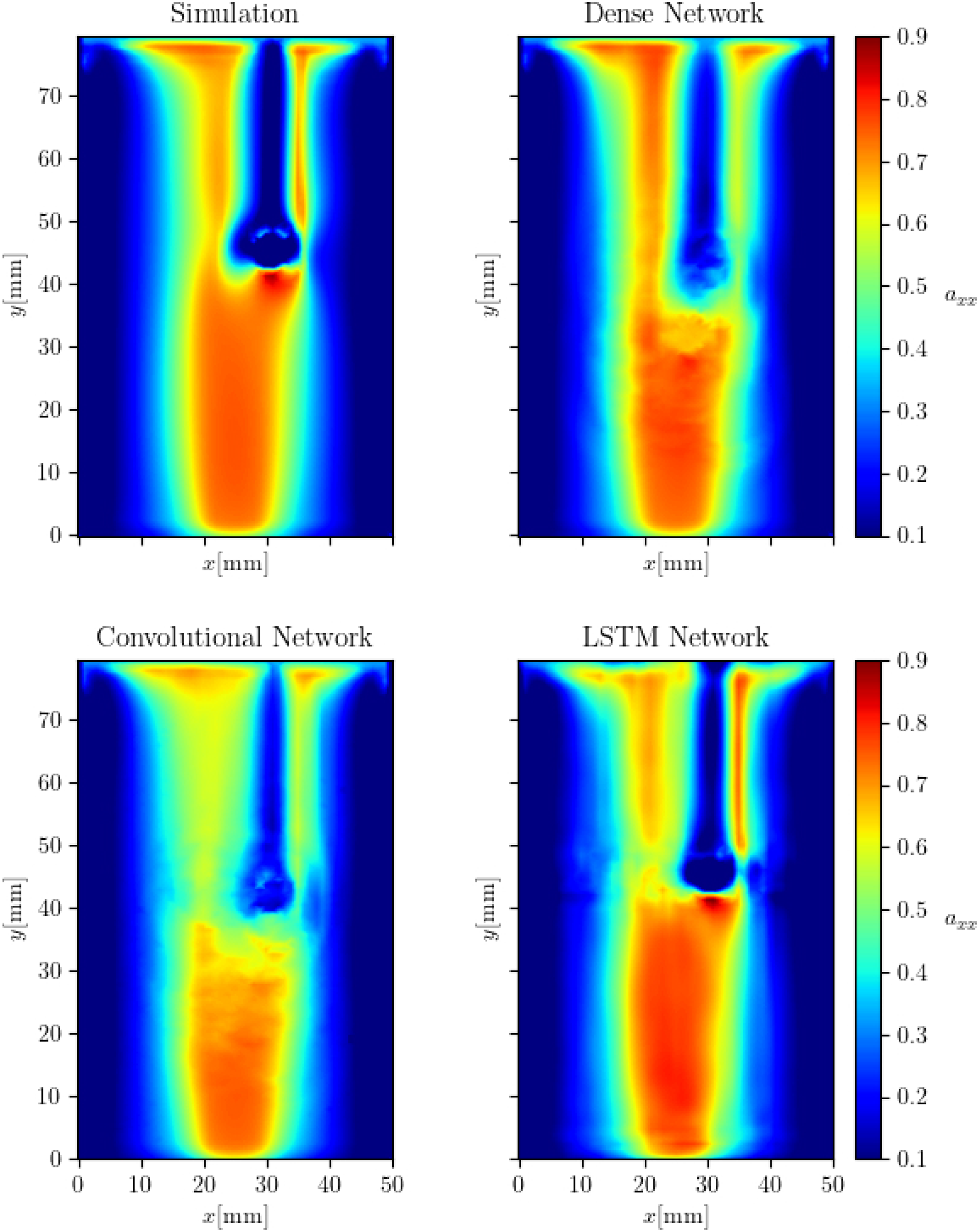
To gain a better understanding on how good the capabilities of the different models are, their predictions of individual plates are visualized in Figure 10 for a plate from the training set and in Figure 11 for a plate from the validation set. Again visualisation is done from a top-down perspective of the midmost elements in thickness direction with the color code for the A_xx component showing the tendency of the fibers to align with the x axis.

Figure 10.

A comparison of the predictions of the trained NN with the simulated data of a plate from the training data.

Figure 11.

A comparison of the predictions of the trained NN with the simulated data of a plate from the test data.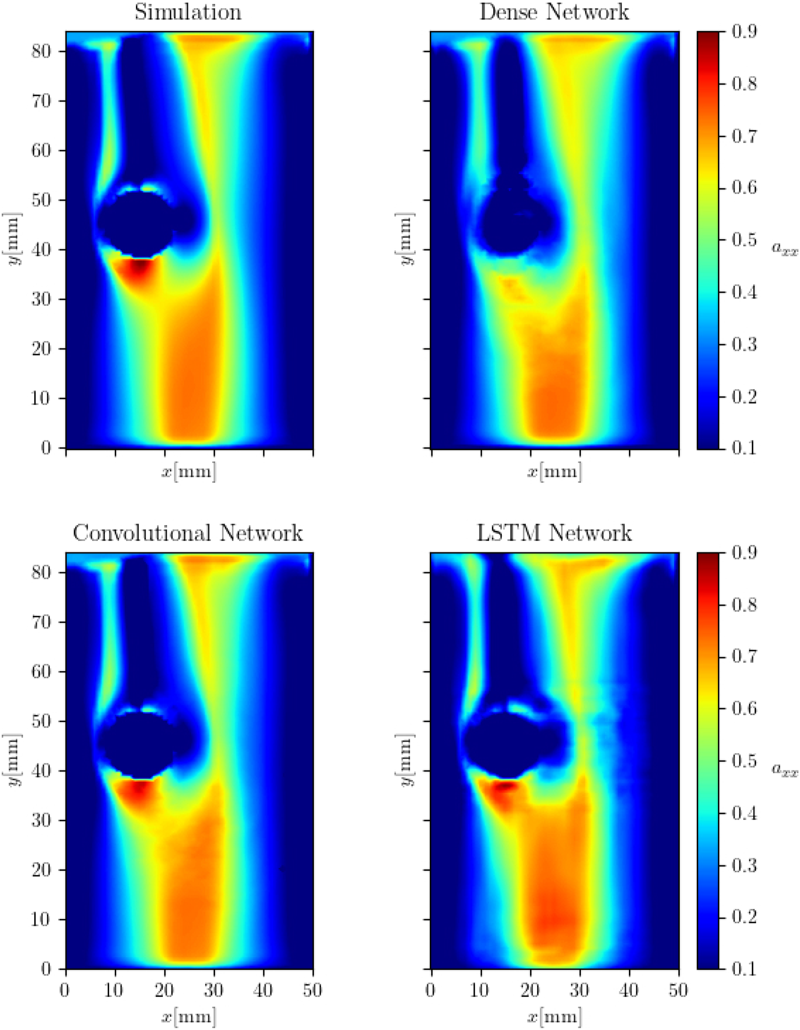

Regarding the training example, all models successfully grasp the major characteristics of the simulations: including the influence of the dice walls, the accumulation at the end of the plate, the cut-through area, the flow pattern around it, and the unoriented fibers in the weld line behind the hole. The dense networks prioritises the overall trend of the fibers over intricate details, as for example the sharp transitions near the hole. In contrast, the LSTM network also captures the more distinct features but exhibits increased noise in the distribution, especially at the edges of the patterns. Lastly, the convolutional network provides outstanding predictions, presenting almost perfect copies of the simulations.

Even more significant is the capacity of the models for predicting new data, as this is the ultimate objective of models trained to partly replace simulations and speed up the molding prediction. For the unfamiliar data, the convolutional network cannot maintain the previously demonstrated superb results, performing significantly worse in terms of grasping the distinct features of the simulated FOTs, also failing to predict the broader trend for some areas. The dense network presents similar forecasts. The LSTM network exhibits superior outcomes for both the validation and the test instances, effectively capturing patterns and the overall trend.

Conclusion

This study demonstrates that NN can be trained on molding simulations to predict the local fiber orientation of SFRP and account for the influence of the component geometry. The three tested architectures exhibit good results and are capable to predict the largest of the FOTs for the chosen geometry (with MSE < ${10}^{-2}$ ). All of them demonstrate the potential for significant decreasing the computational expenses for forecasting, speeding the process up by a factor of 10,000. Thereby NN achieves the goal of creating a prediction within minutes even for large components. The best performing architecture is the LSTM, presenting the lowest MSE on all datasets ( $7\times {10}^{-4}$ and $2.5\times {10}^{-3}$ ) and demonstrating excellent pattern forecasting, including on unseen data. Despite taking 23h to train the model, for predicting it outperforms traditional methods by a magnitude of ${10}^4$ . The CNN performs exceptionally well on the training data ( $1.8\times {10}^{-3}$ ) while having trouble capturing the visible patterns of the plates the model was not optimized for during the learning cycle. Lastly, the DNN shows decent and consistent results, especially in comparison to the minimal computational demands of the model.

Seeing the advantages of AI, it is important to keep in mind, that with the presented method there will always be a need for the traditional methods of molding simulation. For once, as creating an experimental data base is far too much effort, all AI must be built on simulative results and therefore can not be better than the simulations. And secondly, the implementation of new features observed in experiments or even the modeling a different material cannot be done by only NN but needs the creation of a data basis with detailed simulations.

The presented method shows that NN will play an indispensable role in molding simulations in the future. There are however several ways the method could be improved and extended. The input features applied here were very much suitable for the simple geometry. But for more diverse and general geometries the input features should be more transferable between use cases. Similarly, in this research all plates were mapped on a grid with equal size. But in practice there will be different input dimensions for different geometries, raising the need for flexible architectures.

Overall, the presented method and results show that NN can be applied to predict the FOTs in a molding process. It has great advantages by reducing the prediction time while relying on the traditional method for creating a training data basis. With a larger data basis more specialized network architecture could be developed enabling the application to real components and revolutionizing the whole field of molding simulations.