Sage Journals: Discover world-class research

Abstract

The prerequisite to equip structures with in situ electrical health monitoring systems in a meaningful manner is to estimate potential damage locations. In this context, an analytical approach to model the spatial and temporal evolution of transverse inter-fibre fractures (IFF) is exemplified for ${[90_{3} / 0_{2}]}_{s}$ cross-ply laminates under three-point bending. The model is based on the tensile load in the bottom 90°-layer. The effective stress is computed directly from the specimen displacement, whereas the strength is considered to be periodically distributed due to material inhomogeneities along the specimen. The continuous comparison between the sinusoidal strength function and the effective stress allows modelling progressive damage in form of IFF. A modified Hann window is used to consider their effect to the bottom 90°-layer. Experiments with the same configuration are performed and the observed IFF evolution is used to tune the model parameters in an optimisation procedure, e.g., the peak separation of the sinusoid and the length of the Hann window. The comparison between model and experiment shows a high level of agreement. The model is thus capable to reproduce experiments with minimal computational effort. This makes it highly suitable as input for electrical monitoring models that rely on the continuous damage evolution of the investigated structure. In its current form, the model is limited to the specified configuration. However, the simple analytical approach allows it to be easily adapted. It is furthermore shown that progressive composite damage in terms of spatial and temporal evolution can be accurately described using an analytical approach.

Keywords

Analytical model carbon fibre reinforced polymer inter-fibre fracture parameter optimisation three-point bending

Introduction

Carbon fibre reinforced polymers (CFRP) are a preferred material in aerospace and automotive applications where light weight and durability are required in addition to mechanical integrity under continuous load cycles. In order to use CFRP structures more extensively in load-bearing conditions, the monitoring for structural failures in an economical manner is essential. Therefore, it is crucial to develop built-in sensing systems that allow continuous monitoring of the integrity of structures, thus enabling Structural Health Monitoring (SHM). SHM can be performed using e.g. optical fibre bragg grating sensors, infrared thermography testing,^1–3 lamb wave based scanning techniques,⁴ or ultrasonic arrays.⁵ In the case of CFRP, electrically conductive carbon fibers are present in the structure, so that any damage that occurs can be detected via the measurable change in electrical properties.^6–9

In any case, knowledge of possible damage locations and the development of damage over time is advantageous in order to integrate suitable measuring devices into the structure in a meaningful way. The location of the first occurring damage and the further development of damage depend in a specific manner on the considered structure and the loading. However, universally applicable criteria and methods are available that allow these data to be computed or experimentally determined for arbitrary structures. In 1981, Hashin¹⁰ derived criteria for the failure in undirectional fibre composites under different loading conditions and separately modeled fibre and matrix damage modes. In the 1980s and 1990s, early analytical^11,12 and numerical^13,14 models were derived to capture transverse matrix cracking of composite cross-ply laminates under uniaxial tension. Since then different kinds of damage formulations with a varying degree of complexity were developed for composite laminates and are applied in the recent literature.^15–17 Based on these damage formulations, the progressive fracture in composite laminates can be computed. The main focus is on the delamination of single composite layers^18–20 and on the matrix cracking.^21–24 Typically, experimental and numerical methods are used in these works, individually and in combination. However, the numerical computation of multiple damage locations with explicit modeling of the microstructure is time-consuming.²⁵

In this work, the identification of potential damage locations and the development of damage will be exemplified analytically using a CFRP beam consisting of a ${[90_{3} / 0_{2}]}_{s}$ cross-ply CFRP laminate. The laminate layup is selected deliberately, so that any formed IFF is stopped at the lower 90°-0°-layer interface and does not lead to a failure of the entire specimen. The analytical model in its current form is limited to such layups. The question of where cracks form in the bottom 90°-layer of the laminate, how the stresses in this layer change as a result of crack formation, and what crack configuration is formed until failure is investigated. Existing criteria mentioned above for analysing matrix cracks under local stress are utilised using a maximum allowable stress criterion. Furthermore, it is assumed that material inhomogeneities in the laminate are involved in the matrix cracking behaviour,^26–29 i.e., in the formation of inter-fibre fractures (IFF). These inhomogeneities may be present directly in the material, or may be a result of the manufacturing process. Thus, the material properties of the composite, in the present case strength as the maximum allowable stress, are considered to have a spatial distribution.^29,30

An analytical model for this structure is developed, numerically evaluated and experimentally verified. For this purpose, a three-point bending test is used. Compared to a tensile test as an alternative, it results in clearly distributed IFF on just one side of the specimen. For the proposed model, the three-point bending configuration is further advantageous over a four-point bending configuration characterised by a sectionwise constant normal stress because an individual value of the normal stress is allocated to each position over the half-span of the specimen. This allows the highly accurate and temporally unambiguous identification of IFF during the experiment and provides reliable inputs for the introduced model. The above-mentioned properties are implemented in the model of the laminate, which is thus able to provide data on the spatial and temporal evolution of matrix damage in the lower layer of the CFRP cross-ply laminate. In this way, indications are obtained as to where measuring devices should be installed to monitor the structural condition. Experimental reference data from an earlier work of the authors²⁴ are used to tune the model parameters in an optimisation process.

The above should make it clear that the procedure described can be useful when designing structures that are to be equipped with SHM systems. The prerequisite is the existence of a model for the mechanical structure, an analytical or numerical model for the initiation and development of damage and, if necessary, an assumption about the spatial distribution of the material strength. The methodology used and the procedure explained here as an exemplary case can then be transferred to other structures, systems and laminate layups with 90°-layers.

The remainder of the manuscript is organised as follows. First, the authors’ experimental results, see also Linke et al.²⁴, are briefly revisited. This is followed by the presentation of the analytical model of the mechanical system. Here, the stress distribution, the spatially heterogeneous distribution of strength and the modeling of the inter-fibre fractures are discussed. In the next section, the parameters included in the model are determined by an optimisation procedure. Finally, the results obtained with the model and the optimised parameters are presented and compared with experimental results. The main results of the work are summarised at the end.

Experiments

This section details the specimen manufacturing and the experimental procedure used for data collection. The information given in this section has been adopted from an earlier work of the authors.²⁴

Specimen manufacturing

The specimens for this work are manufactured from prepregs (Hexcel HexPly M21/34%/UD194/T800S) with an epoxy matrix and unidirectional carbon fibre reinforcement. Multiple plies of the prepreg are stacked in ${[90_{3} / 0_{2}]}_{s}$ sequence. The laminate is cured under 7 bar pressure at 180°C for 120 min in an autoclave with nitrogen atmosphere. After curing, the laminate is cut into specimens with dimensions of 100 mm × 15 mm using a water-lubricated diamond saw. The specimens are cleaned by using isopropyl alcohol in order to remove any loose particles from the cutting processes. No further polishing is performed. The nominal thickness h is 1.9 mm (see Figure 1). A total of four specimens are manufactured. Since inhomogeneities, e.g., voids and resin-rich areas, are expected to affect the mechanical response and thus the experimental results,^30–32 testing multiple specimens increases the significance of the obtained data. However, the parameters of the introduced analytical model are tuned in order to fit it to an arbitrary experimental reference. Hence, the general applicability of the model and of the optimisation procedure is independent from the number of performed experiments.

Figure 1.

Specimen configuration for experimental testing and analytical modeling.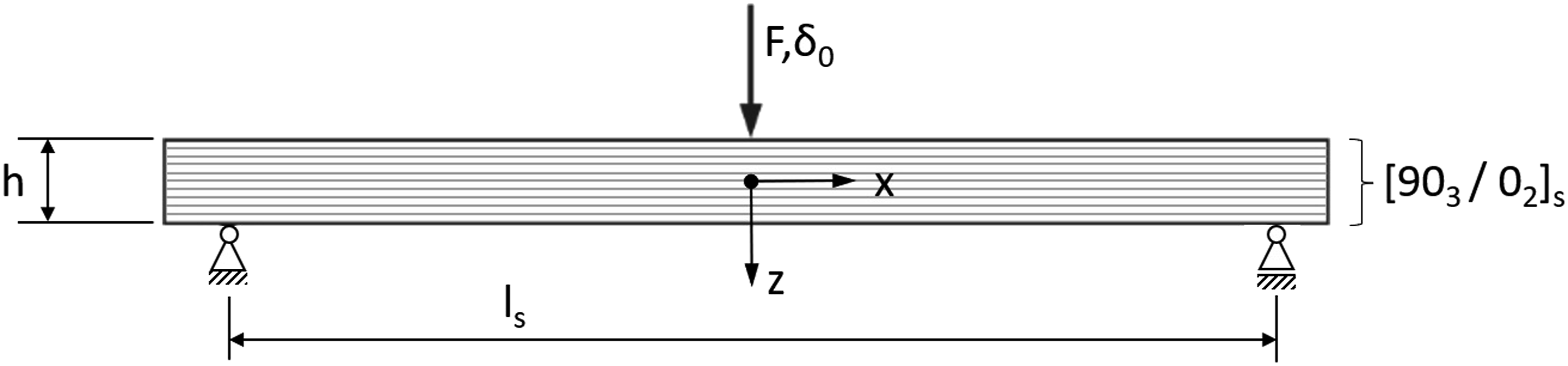

Setup and procedure

Prior to test, the specimens are observed with a Keyence VHX-5000 digital microscope to locate potential pre-cracks from the manufacturing process. For the four specimens tested, an amount of zero, one, two and four pre-cracks per specimen is detected. The three-point bending test is performend on a Tira Test 2810 testing machine. Supports of radius 2 mm and a 1 kN load transducer with a mandrel radius of 5 mm are employed. The support span l_s is 55 mm and the velocity of the mandrel is set to 5 mm/min. Relevant data about time T, displacement of the mandrel δ₀ and applied force F are sampled at a rate of 50 Hz. The specimens are not loaded to ultimate failure in order to avoid extensive permanent deformation. Only displacements δ₀ ≤ 8.5 mm are used for evaluation. The specimen configuration with the origin of the xz-coordindate system in the centre is shown in Figure 1.

An infrared camera VarioCam from Infratec is installed at a distance of 100 mm from the side face of the specimen. It observes the experiment for potential IFF, that form at the bottom face of the specimen. The mechanical energy, that is introduced through the mandrel, is partially transformed into thermal energy and released during IFF formation. The increased temperature around an IFF, which is about 0.32 K,²⁴ can be detected using passive infrared thermography (PIRT). PIRT images are logged with a rate of 12 Hz and provide information about time of occurence T_IFF as well as about the approximate horizontal position of new IFF. However, the deformation of the specimen is not considered in this measurement. After test, the specimens are observed again under the optical microscope to obtain the exact, individual position x_IFF of every IFF that occured during the experiment. Previous data about pre-cracks are removed from the data set. In accordance with the reason for the selection of ${[90_{3} / 0_{2}]}_{s}$ laminates, all formed IFF travel completely through all bottom 90°-layers and stop at the 90°–0°-layer interface. No delaminations are observed at this interface.

Post-processing

In order to relate spatial (x_IFF) and temporal information (T_IFF) for each IFF, gathered data from the experiments are correlated. First, the approximate positions from PIRT are corrected with respect to the displacement δ₀ of the specimen using a function as introduced by Linke et al.²⁴ Second, the true IFF position x_IFF along the specimen from microscopic analysis is correlated with the temporal information T_IFF from PIRT. Finally, this temporal information T_IFF is correlated to force and displacement data (F-δ₀) from the testing machine that are logged in discrete time steps. Thus, a complete picture of the spatial and temporal evolution of IFF in a CFRP specimen under three-point bending can be gathered that additionally provides information about mandrel displacement δ₀ and applied force F in the moment of IFF formation.

Modeling

In this section, a first approach to model the IFF formation in the bottom 90°-layer of laminates under a three-point bending test is derived. This approach is based on two analytical functions. The first one describes a periodically varying function for the maximum allowable stress to consider material inhomogeneities. The second one applies a window function to the triangular normal stress distribution in bent beams to incorporate the impact of formed IFF.

Homogeneous normal stress distribution

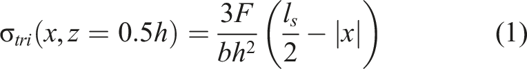
Formation of IFF in specimens is caused by local tensile stresses exceeding a maximum allowable stress σ_max(x). For the given configuration (see Figure 1), tensile stresses occur in the lower half of the deflected specimen. The effective stress directly depends on the local bending moment within the support span l_s. It increases linearly (a) from the supports to the load introduction point, (b) from the horizontal symmetry plane of the laminate to the bottom 90°-layer via position z [−0.5 h ≤ z ≤ +0.5 h] and (c) with the applied force F.^33–35 Since solely the stress at the bottom of the laminate is considered, z has a fixed value of 0.5 h. The resulting stress between the supports has the theoretical shape of a triangle. This triangular stress σ_tri(x) is given by

σ_{t r i} (x, z = 0.5 h) = \frac{3 F}{b h^{2}} (\frac{l_{s}}{2} - | x |)

(1)

where x has its origin in the centre of the specimen, h is the thickness and b the width of the specimen.^33,36 The triangular stress σ_tri(x) is proportional to the applied force F which is related to the centre displacement δ₀ via recorded test machine data as displayed in Figure 2. The third-order regression function

F (δ_{0}) = - 0.0028 \frac{N}{{m m}^{3}} \cdot δ_{0}^{3} - 0.8647 {\frac{N}{m m}}^{2} \cdot δ_{0}^{2} + 34.8879 \frac{N}{m m} \cdot δ_{0}

(2)

is obtained from all performed experiments. It is clearly evident that the function becomes increasingly non-linear for large displacements δ₀. This is due to the effect of IFF formations in the specimens.

Figure 2.

Experimental force–displacement curves of four specimens (black) and regression function (red).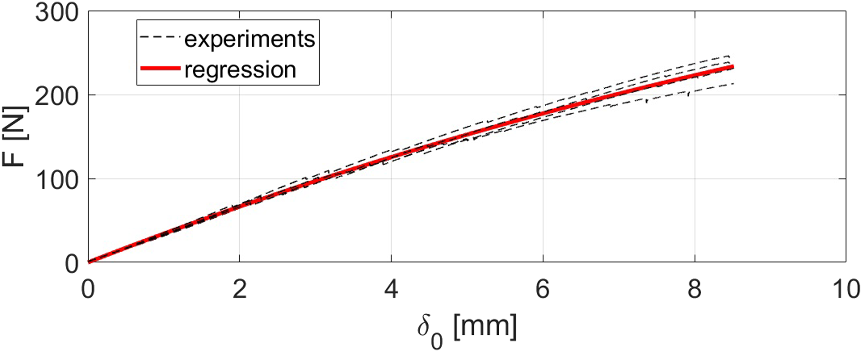

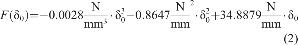
The applied force F is then plugged into equation (1) to make the triangular stress σ_tri(x) dependend on the applied displacement δ₀. The maximum displacement δ_0, max is set to a nominal value of 8.51 mm which is the maximum covered by all the experiments.

Since the modeled system is statically determined (see Figure 1), there is no load redistribution after fracture.

Heterogeneous strength distribution

For a general imperfect specimen, as assumed in this work, randomly dispersed inhomogeneities such as voids, pre-cracks or resin-rich areas^37–39 must be considered for the modeling process. They can affect the local damage formation threshold, e.g., the maximum allowable stress or strain.^29–31 It is reported in the literature that the stochastic distribution of these intrinsic properties in the specimen has not necessarily a monotone trend.²⁹ Arai et al.³⁰ numerically obtained a non-uniformal distribution of the maximum stress in FRP and assumed, among others, a periodic microstructure. The current work takes up this approach and models the strength of the heterogeneous specimen via a periodic and harmonic sinusoid as given by

σ_{\max} (x) = σ_{def} + σ_{A} \cdot \sin (2 π \frac{x}{λ} + ϕ)

(3)

that depends on the defect threshold σ_def, the peak amplitude σ_A, the peak separation λ and the offset ϕ. It takes into account stochastically distributed variations from the nominal defect threshold σ_def. The selected sinusoid is a first approach to model these variations. The experimentally observed fact that an IFF can form at a lower x position after another IFF formed at a higher x position indicates that a homogeneous strength is not able to model the IFF evolution sufficiently. Due to its nature, a constant strength value in combination with the triangular stress distribution can only capture IFF formation with increasing x positions. Thus, a superposed function that locally varies the strength as a function of x is required, so that the specific IFF evolution from the experiments can be modeled. However, a variety of other functions σ_max(x) may be applied.

Modeling of IFF

The model in the unloaded condition (δ₀ = 0 mm) is depicted Figure 3(a). In this state, the effective stress distribution σ_eff(x) is equal to the triangular stress σ_tri(x). It is important to note that the presence of pre-cracks is neglected in the current approach since the model aims to consider the mean experimental behavior from four tested specimens. The latter are characterised by individual amounts and positions of pre-cracks. In the course of the simulation, the model continuously compares the increasing effective stress σ_eff(x) with the sinusoidal strength σ_max(x) over the length of the specimen [−1/2l_s ≤ x ≤ +1/2l_s]. An IFF forms at x = x_IFF, when the stress locally exceeds the strength: σ_eff (x_IFF) > σ_max (x_IFF), see Figure 3(b) and (d).

Figure 3.

Visualisation of the triangular stress σ_tri(x) and the effective stress σ_eff(x) compared to the modeled strength σ_max(x) for increasing displacements δ₀ and number of IFF. All model parameters have an exemplary setting. (a) δ₀ = 0.00 mm: No effective stresses σ_eff(x) are present in the specimen. The strength σ_max(x) is periodic. (b) δ₀ = 2.03 mm: The first maxima (marked by ○) of the effective stress σ_eff(x) reaches the modeled strength σ_max(x). (c) δ₀ = 2.04 mm: Formation of the first IFF forces the local stress σ_eff(x) to zero and affects the stress in the vicinity. (d) δ₀ = 2.62 mm: Another maxima (marked by ○) of the effective stress σ_eff(x) reaches the modeled strength σ_max(x).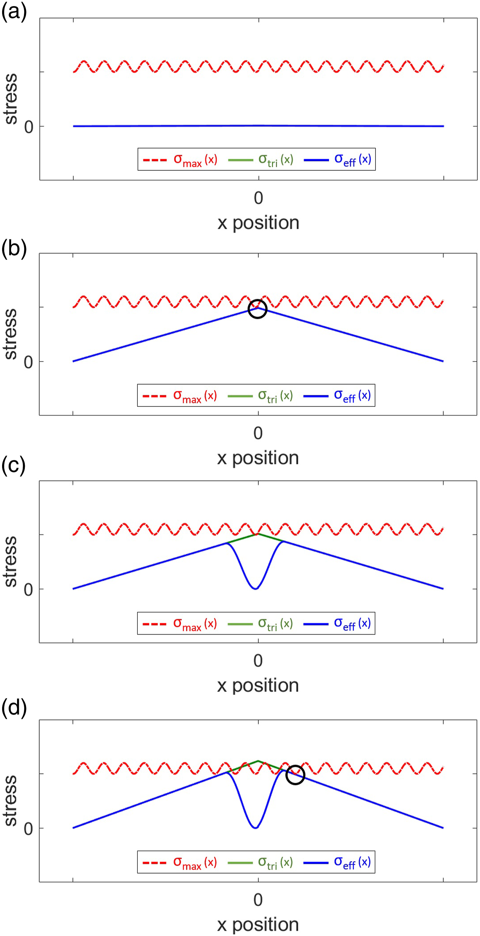

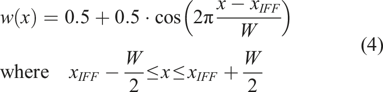
As the considered bottom layer of the composite fails, the effective stress σ_eff(x) at the IFF location x_IFF must be forced to zero.^40–42 To model this constraint, a modified Hann window

\begin{array}{l} w (x) = 0.5 + 0.5 \cdot \cos (2 π \frac{x - x_{I F F}}{W}) \\ w h e r e x_{I F F} - \frac{W}{2} \leq x \leq x_{I F F} + \frac{W}{2} \end{array}

(4)

is introduced.^43–45 Contrary to the original definition of the Hann window, this function ranges from one at its edges to zero in the centre of the window. It models a section of length W with reduced stress in the vicinity of the IFF, see Figure 3(c). Each time a new IFF (counting number n) occurs, the modified Hann window w(x) is locally applied to the effective stress σ_eff(x) in the affected interval

[x_{I F F, n} - W / 2 \leq x \leq x_{I F F, n} + W / 2]

Parameters

The presented modeling approach for the IFF evolution requires five input parameters. The following parameters characterise the sinusoidal strength σ_max(x): (1) the defect threshold σ_def offsets the baseline of the sinusoid along the stress axis, (2) the peak separation λ defines the distance in space between two adjacent strength maxima, (3) the peak amplitude σ_A sets the extremal values with respect to σ_def and (4) the offset ϕ shifts the periodic function along the longitudinal specimen axis starting from the centre. Further, (5) the length of the window W characterises the size of the reduced stress section in the vicinity of an IFF. These parameters are shown in Figure 4.

Figure 4.

Visualisation of the model including parameters to be optimised.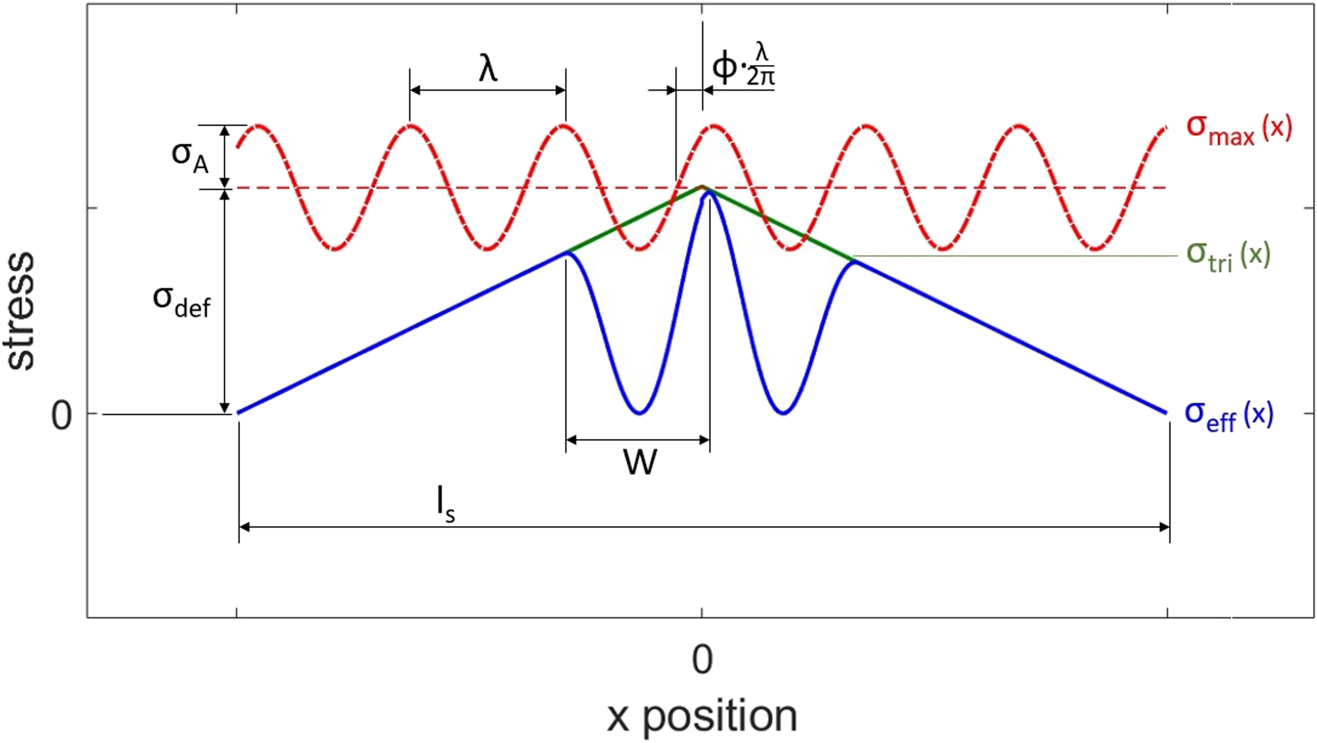

Parameter optimisation

In this section, an approach for the parameter optimisation is outlined. First, reasonable settings are selected for all model parameters based on mechanical considerations. The analytical model is then run for the chosen variety of parameter settings. To evaluate the model and to find the optimised settings, two figures of merit are introduced that consider the spatial distribution and the number of IFF at every displacement δ₀. Finally, the optimised parameter set is discussed.

Parameter settings

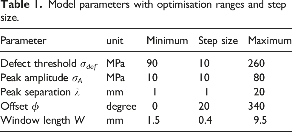
The ranges and the step sizes for the model parameters used for optimisation are selected considering simple constraints, e.g., the peak amplitude σ_A must be smaller than the defect threshold σ_def and the peak separation λ should be far smaller than the support span l_s. The defect threshold σ_def is approximated using experimental IFF information and the triangular stress σ_tri(x).

The required model parameters and their selected settings are listed in Table 1. In the context of the optimisation process, all possible combinations of these parameter settings are used as an input for the model. After each run, the figures of merit introduced in the following are applied to the results in order to evaluate the agreement with the experimental reference data. It has to be noted that the goal of this work is to describe an analytical approach that reasonably models the IFF evolution in bent CFRP specimens. A more detailed optimisation strategy that may result in a lower overall error is beyond the scope this paper.

Table 1.

Model parameters with optimisation ranges and step size.

Parameter	unit	Minimum	Step size	Maximum
Defect threshold σ_def	MPa	90	10	260
Peak amplitude σ_A	MPa	10	10	80
Peak separation λ	mm	1	1	20
Offset ϕ	degree	0	20	340
Window length W	mm	1.5	0.4	9.5

The optimised parameter settings will give an idea of the magnitude of each parameter and how the ultimate settings might be. Further, these settings will allow conclusions about the significance of each parameter on the model output and how they affect the latter.

Figures of merit

The optimisation of the model parameters is performed with experimental data as reference. Two different figures of merit are used. They are easily to determine and characterise the spatial and temporal IFF evolution. The first one is the current number of IFF (NOI). The second one is the IFF distribution width (IDW) which is the distance between the rightmost and the leftmost IFF at a particular displacement δ₀.

To compare information about these figures of merit, two aspects must be considered. (I) Since NOI and IDW are measured in different units, a relative measure has to be introduced. (II) The mean values of the associated quantities over the entire experiment, 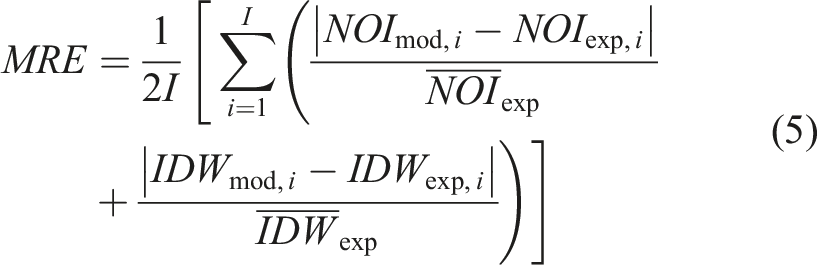${\bar{N O I}}_{\exp}$ = 5.14 and ${\bar{I D W}}_{\exp}$ = 16.09 mm, are used to obtain the relative errors. This ensures equal reference values for the errors troughout the experiment. Finally, the errors for NOI and IDW over all displacements δ_0,i (increment size Δδ₀) are equally weighted to obtain a final mean relative error (MRE) of the model. It is defined as

M R E = \frac{1}{2 I} [\sum_{i = 1}^{I} (\frac{| N O I_{\mod, i} - N O I_{\exp, i} |}{{\bar{N O I}}_{\exp}} + \frac{| I D W_{\mod, i} - I D W_{\exp, i} |}{{\bar{I D W}}_{\exp}})]

(5)

where I = δ_0, max/Δδ₀ is the number of evaluation points. Experimental reference data NOI_exp,i and IDW_exp,i are obtained by calculating the mean values from all four experiments at the associated displacement δ_0,i.

Results of the optimisation

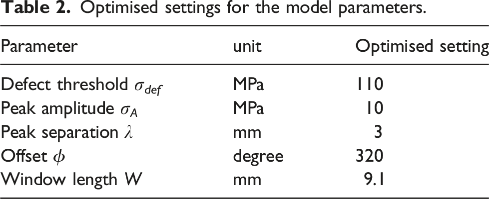
The optimised parameter settings based on the introduced figures of merit are listed below in Table 2. A minimum MRE of 7.70% is achieved with this combination, which results from an error of 9.85% for NOI and 5.55% for IDW, respectively. Basically, the optimised settings are only valid for the investigated three-point bending configuration. The applicability to other configurations needs to be addressed in a subsequent work. However, the method used can be adopted.

Table 2.

Optimised settings for the model parameters.

Parameter	unit	Optimised setting
Defect threshold σ_def	MPa	110
Peak amplitude σ_A	MPa	10
Peak separation λ	mm	3
Offset ϕ	degree	320
Window length W	mm	9.1

The model output as a result of the optimisation is plotted in Figure 5. Good agreement with the experimental average over the entire experiment is achieved. The vast majority of the data points are within the experimental boundaries, shaded in grey.

Figure 5.

Comparison between experimental data and analytical model as a result of the optimisation process. (a) Comparison of the number of IFF (NOI), (b) Comparison of the IFF distribution width (IDW).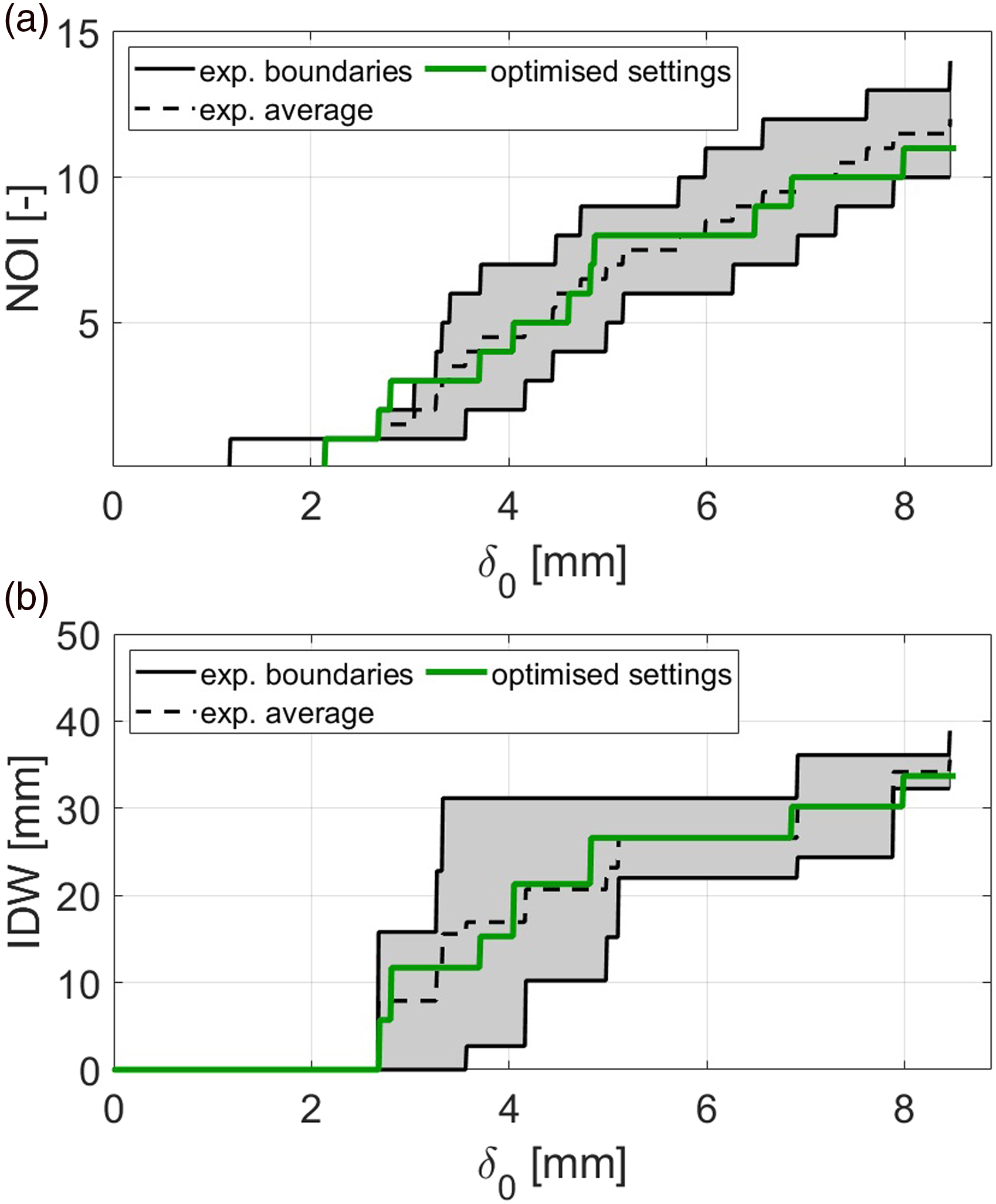

The results reveal some interesting aspects about the model. First, the optimised parameters for the peak amplitude σ_A = 10 MPa and the defect threshold σ_def = 110 MPa show that the main contribution to the strength σ_max(x) comes from the latter. This is in accordance with the general idea of the modeling approach that a constant defect threshold is superposed with a moderate spatial variation due to inhomogeneities. This variation σ_A is around 9% of the base value σ_def. Thus, the material inhomogeneity is assumed to be relatively small.

Secondly, the optimised length of the window W is found to be 9.1 mm. This is more than a factor of 2.5 larger than the mean IFF spacing of 3.39 mm determined during the experiments.²⁴ The analytical model thus reveals that the window length W does not constrain the IFF spacing. New IFF can rather form within the weakened section around an extisting IFF. The reason for this behaviour is the application of the modified Hann window w(x) itself, which introduces an extra local maximum to the effective stress σ_eff(x) (see Figure 3(c)) where new IFF may form.

Moreover, the combination of the peak separation λ = 3 mm and the offset ϕ = 320° gives the first IFF at x_IFF = −0.4 mm. This is consistent with experimental observations that the first IFF occurs near the specimen centre.²⁴ Further, Figure 6 shows the effective stress σ_eff(x) at the end of the simulation. The IFF positions are nearly uniformly distributed along the x-direction of the specimen. Their spacing mainly ranges from 2.7 mm to 3.6 mm, just one value of 5.3 mm is higher than the others. The resulting mean IFF spacing of the model is 3.37 mm, which is very close to the experimental reference value. It clearly correlates with the optimised setting for λ = 3 mm. The latter thus mainly defines the IFF spacing of the model. Accordingly, the offset ϕ defines the position of the first IFF based on the obtained peak separation λ.

Figure 6.

Effective stress σ_eff(x) at the end of the simulation (δ₀ = 8.51 mm) with optimised parameters. IFF positions are marked with a black square.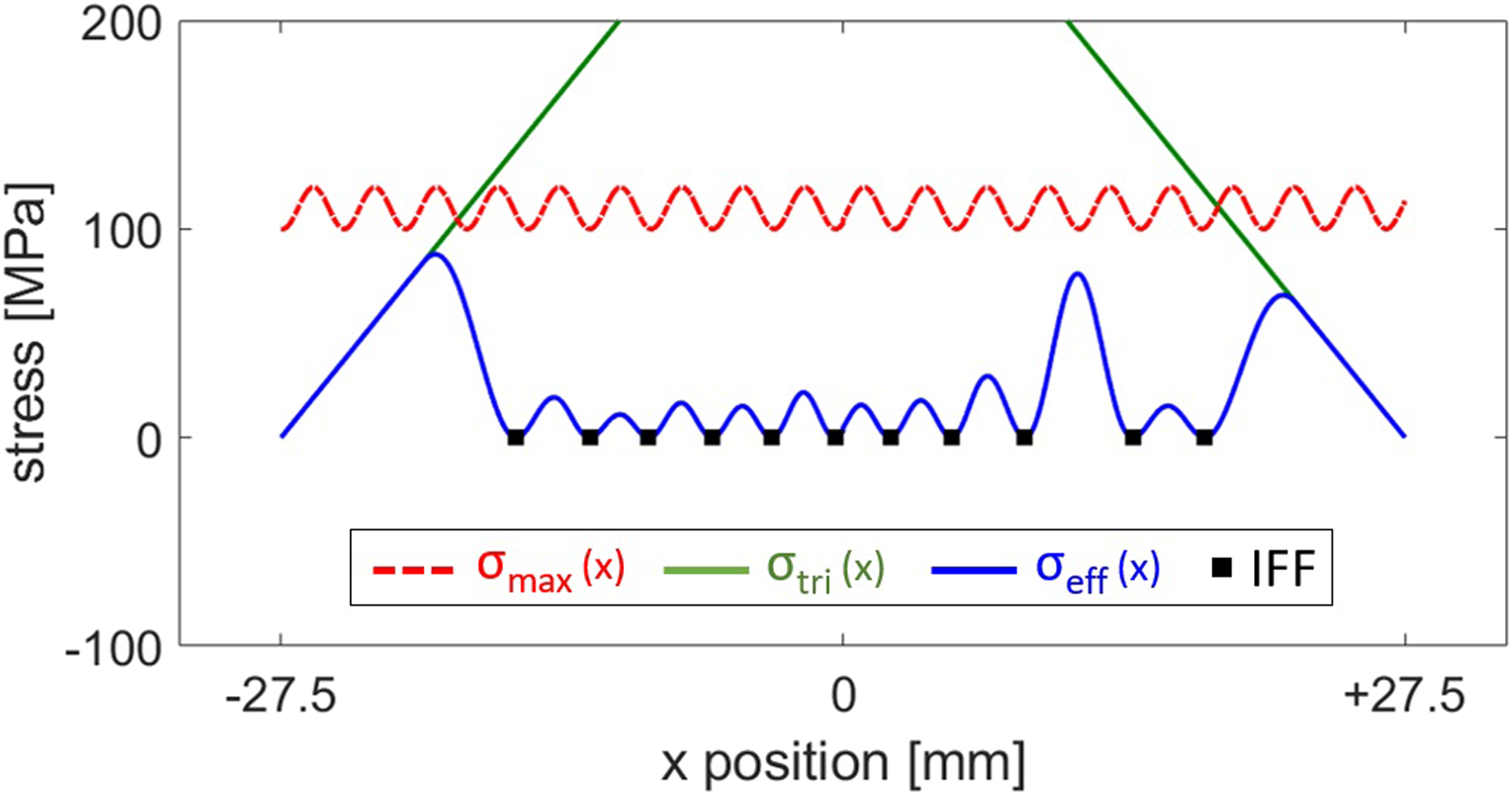

Finally, Figure 6 shows the increasing weakening effect due to existing IFF. The triangular stress σ_tri(x), which assumes an undamaged specimen, exceeds the strength σ_max(x) over a wide range (approximately 67% of the support span l_s). It outlines the necessity of the modified Hann window w(x) that significantly reduces the effective stress σ_eff(x) in order to fit the simulation with the experiment for increasing damage.

The model with optimised parameters shows good agreement with the experimental data in Figure 5 that are included in the figures of merit for the optimisation process. In addition, the model confirms the experimental observation that the first IFF forms near the specimen centre. Further, the mean experimental IFF spacing matches the analytically obtained value. The latter directly results from NOI and IDW. In this context, Figure 7 compares the IFF evolution in terms of the position x and the critical displacement δ₀ as a result of the analytical model (a) with the experimental data (b-e) from four experiments. The plots further reveal the NOI, the IDW as well as the IFF spacing. It is evident that qualitative agreement with respect to the spatial and temporal evolution is achieved. Thus, the presented analytical approach, characterised by a sinusoid-based and heterogeneous strength distribution, and the selected figures of merit are found to be well suited to model the spatial and temporal IFF evolution in ${[90_{3} / 0_{2}]}_{s}$ cross-ply laminates under three-point bending tests. However, a direct comparison between the analytical model and a single experiment is not reasonable since the model with calibrated parameters represents the mean IFF evolution over a variety of experiments.

Figure 7.

Output of the analytical model and data from four experiments with respect to the position x and the critical displacement δ₀ for each IFF. (a) Analytical model, (b) Experiment #1, (c) Experiment #2, (d) Experiment #3, (e) Experiment #4.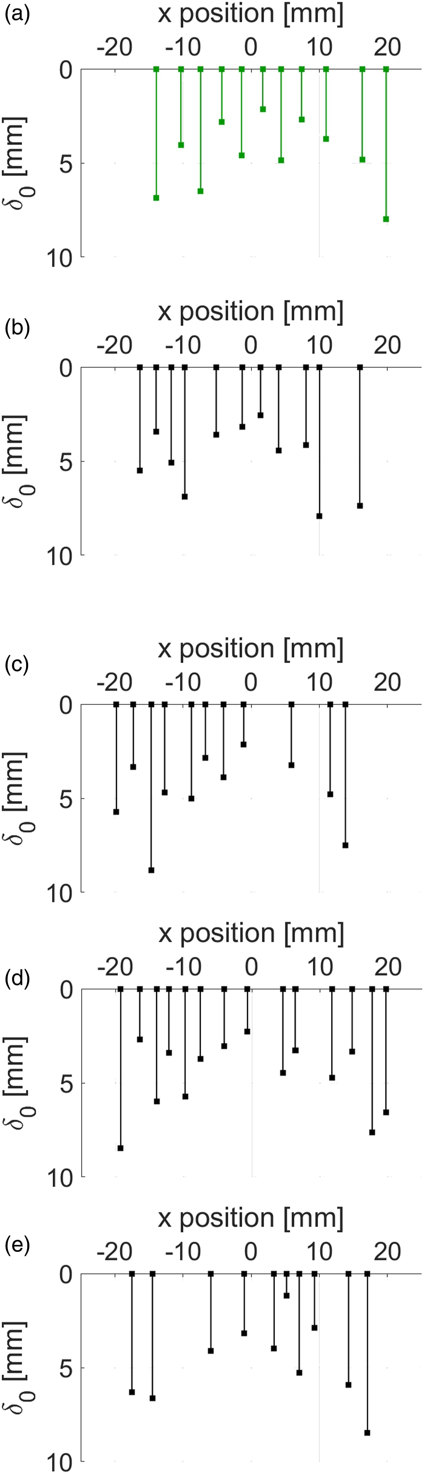

Conclusion

In this paper, an analytical approach to model the IFF distribution in the bottom 90°-layer of ${[90_{3} / 0_{2}]}_{s}$ CFRP laminates under a three-point bending test was outlined. It was based on two concepts. First, the maximum allowable tensile stress before IFF formation was modeled periodically distributed along the longitudinal specimen axis using a sinusoid. Secondly, the effective tensile stress at the bottom of the specimen was assumed to have a basic triangular function and formed IFF were considered via a modified Hann window to account for the continuous weakening effect. It was shown that optimisation can be used to tune the parameters of the model and to find good fit with experimental results. Further, correlation between model parameters and experimental characteristics were identified, e.g. between the peak separation and the mean IFF spacing. However, the analytical model and the optimised parameter settings in their current form are limited to IFF formation in the bottom 90°-layer of ${[90_{3} / 0_{2}]}_{s}$ laminates under a symmetrical three-point bending experiment. The application to other configurations, such as different force–displacement curves, support spans, asymmetrical load introduction or laminate layups including 90°-layers, needs to be investigated in a subsequent work that requires additional experimental data for validation. However, the advantage of the modeling approach is its simplicity and its flexibility to be generally adaptable to these configurations. The derived significance of the model parameters indicates that they have a physical background and may be transferred to varying experimental reference data. Improvements to the model could be achieved via implementation of the effect of pre-cracks to the initial stress distribution. However, in this case only a single experiment can be used as reference due to the distinct allocation of amount and position of pre-cracks. In its current form, this is not the intention of the model. No other forms of damage such as delaminations or fibre breakage are covered by the analytical model. The prediction of the IFF evolution in CFRP laminates could be used to optimise the location of sensors in order to improve SHM techniques. As the piezo-resistivity of CFRP is understood from the point of view of geometrical and volume changes, a forecast of the IFF evolution under load could supplement existing SHM methods based on sensor networks that rely on electrical resistance change, see e.g. Swait et al.⁴⁶ Further, the generated output can be exploited to built enhanced models that compute the electrical response of the specimen with respect to the IFF evolution. In this context, the IFF evolution could be artificially modified by the purposeful adaptation of the model parameters.

Footnotes

Declaration of conflicting interests

The author(s) declared no potential conflicts of interest with respect to the research, authorship, and/or publication of this article.

Funding

The authors disclosed receipt of the following financial support for the research, authorship, and/or publication of this article: This work was supported by the Deutsche Forschungsgemeinschaft [grant number 3933868053].

ORCID iD

Max Linke

References

Kahandawa

Epaarachchi

Wang

, et al. Use of FBG sensors for SHM in aerospace structures. Photonic Sens 2012; 2(3): 203–214.

Gholizadeh

. A review of non-destructive testing methods of composite materials. Procedia Structural Integrity 2016; 1: 50–57.

Liu

Chung

, et al. Infrared thermography measurement for vibration-based structural health monitoring in low-visibility harsh environments. Sensors 2020; 20(24): 7067.

Diamanti

Soutis

. Structural health monitoring techniques for aircraft composite structures. Prog Aerosp Sci 2010; 46(8): 342–352.

Pan

, et al. Frequency of well-identified oncogenic driver mutations in lung adenocarcinoma of smokers varies with histological subtypes and graduated smoking dose. Lung Cancer 2013; 79: 8–13.

Schueler

Joshi

Schulte

. Damage detection in CFRP by electrical conductivity mapping. Compos Sci Technol 2001; 61(6): 921–930.

Athanasopoulos

Kostopoulos

. Damage detection via Joule effect for multidirectional carbon fiber reinforced composites. Appl Phys Lett 2012; 101(11): 114109.

Nonn

Schagerl

Zhao

, et al. Application of electrical impedance tomography to an anisotropic carbon fiber-reinforced polymer composite laminate for damage localization. Compos Sci Technol 2018; 160: 231–236.

Angelidis

Wei

Irving

. The electrical resistance response of continuous carbon fibre composite laminates to mechanical strain. Compos Part A-Appl S 2004; 35(10): 1135–1147.

10.

Hashin

. Fatigue failure criteria for unidirectional fiber composites. J Appl Mech 1981; 48(4): 846–852.

11.

Ogin

Smith

Beaumont

PWR

. Matrix cracking and stiffness reduction during the fatigue of a (0/90)_s GFRP laminate. Compos Sci Technol 1985; 22: 23–31.

12.

Laws

Dvorak

. Progressive transverse cracking in composite laminates. J Compos Mat 1988; 22: 900–916.

13.

Wang

ASD

Chou

Lei

. A stochastic model for the growth of matrix cracks in composite laminates. J Compos Mat 1984; 18: 239–254.

14.

Guild

Ogin

Smith

. Modelling of 90° ply cracking in crossply laminates, including three-dimensional effects. J Compos Mat 1993; 27(7): 646–667.

15.

Swati

Wen

Elahi

, et al. Extended finite element method (XFEM) analysis of fiber reinforced composites for prediction of micro-crack propagation and delaminations in progressive damage: a review. Microsyst Technol 2019; 25: 747–763.

16.

Deng

Xue

Yin

, et al. A three-dimensional damage analysis framework for fiber-reinforced composite laminates. Compos Struct 2022; 286: 115313.

17.

Shen

Liu

, et al. Progressive failure analysis of laminated CFRP composites under three-point bending load. Adv Mater Sci Eng 2022; 2022: 1–12.

18.

Heidari-Rarani

Sayedain

. Finite element modeling strategies for 2D and 3D delamination propagation in composite DCB specimens using VCCT, CZM and XFEM approaches. Theor Appl Fract Mec 2019; 103: 102246.

19.

Ridha

Chen

, et al. On cohesive element parameters and delamination modelling. Eng Fract Mech 2019; 206: 278–296.

20.

Motamedi

Takaffoli

S Milani

. Nonlinear XFEM modeling of mode II delamination in PPS/glass unidirectional composites with uncertain fracture properties. Materials 2020; 13(16): 3548.

21.

Shi

Soutis

. Modelling transverse matrix cracking and splitting of cross-ply composite laminates under four point bending. Theor Appl Fract Mec 2016; 83: 73–81.

22.

Arteiro

Catalanotti

Reinoso

, et al. Simulation of the mechanical response of thin-ply composites: from computational micro-mechanics to structural analysis. Arch Comput Method E 2019; 26: 1445–1487.

23.

Singh

Vaidya

Thomas

, et al. Finite element modeling of the fiber-matrix interface in polymer composites. J Compos Sci 2020; 4(2): 58.

24.

Linke

Chakraborty

Göbel

, et al. On the accuracy of monitoring inter-fibre fractures in composites using passive infrared thermography extended by microscopic analysis. Nondestruct Test Eva 2021; 36(1): 654–666.

25.

Van der Meer

Sluys

. Continuum models for the analysis of progressive failure in composite laminates. J Compos Mat 2009; 43(20): 2131–2156.

26.

Silberschmidt

. Matrix cracking in cross-ply laminates: effect of randomness. Compos Part A-Appl S 2005; 36(2): 129–135.

27.

Silberschmidt

. Effect of micro-randomness on macroscopic properties and fracture of laminates. J Mater Sci 2006; 41(20): 6768–6776.

28.

Zhu

Zhang

, et al. Influence of voids on interlaminar shear strength of carbon/epoxy fabric laminates. Trans. Nonferrous Met. Soc. China 2009; 19(2): 470–475.

29.

Carraro

Maragoni

Quaresimin

. Influence of manufacturing induced defects on damage initiation and propagation in carbon/epoxy NCF laminates. AMPCS 2015; 1(1): 44–53.

30.

Arai

Fukuda

Sakata

. Random field modeling of microstructure in unidirectional fiber-reinforced plastic using SEM-image and image processing for multiscale stochastic stress analysis considering random fiber arrangements. Adv Eng Mater 2022; 24(5): 2101259.

31.

Sanei

SHR

Jensen

Fertig

. Multiscale stochastic analysis of FRP based on variability in fiber volume fraction, epoxy stiffness and strength. In: 56th AIAA/ASCE/AHS/ASC structures, structural dynamics, and materials conference AIAA 2015, Kissimmee, FL, 5-9 January 2015, 1361.

32.

Rauter

Lammering

. Experimental characterization of short fiber-reinforced composites on the mesoscale by indentation tests. Appl Compos Mater 2021; 28: 1747–1765.

33.

Gross

Hauger

Schröder

, et al. Engineering mechanics 2. Berlin, Germany: Springer, 2011.

34.

Mohyeddin

Fereidoon

. An analytical solution for the large deflection problem of Timoshenko beams under three-point bending. Int J Mech Sci 2014; 78: 135–139.

35.

Troive

. New method for evaluation of bendability based on three-point-bending and the evolution of the cross-section moment. J Phys Conf Ser 2017; 896: 012006.

36.

Altenbach

. Holzmann/meyer/schumpich technische mechanik festigkeitslehre. 11th ed. Wiesbaden, Germany: Springer Vieweg, 2014.

37.

Yang

Boselli

Sinclair

. Simulation and quantitative assessment of homogeneous and inhomogeneous particle distributions in particulate metal matrix composites. J Microsc 2001; 201(2): 189–200.

38.

Paciornik

D’Almeida

JRM

. Measurement of void content and distribution in composite materials through digital microscopy. J Compos Mater 2009; 43(2): 101–112.

39.

Wang

, et al. A mesoscale ultrasonic attenuation finite element model of composites with random-distributed voids. Compos Sci Technol 2013; 89: 44–51.

40.

Abrate

. Matrix cracking in laminated composites: a review. Compos Eng 1991; 1(6): 337–353.

41.

Van den Heuvel

PWJ

Peijs

Young

. Failure phenomena in two-dimensional multifibre microcomposites: 2. A Raman spectroscopic study of the influence of inter-fibre spacing on stress concentrations. Compos Sci Technol 1997; 57(8): 899–911.

42.

Campbell

. Structural composite materials. Materials Park, OH, USA: ASM International, 2010.

43.

Okarma

. Polynomial windows with low sidelobes level. Signal Process 2007; 87(4): 782–788.

44.

Martins

CHN

Silva

LRM

Duque

et al. A new time-varying harmonic decomposition structure based on recursive hanning window. In: 2012 IEEE 15th international conference on harmonics and quality of power, Hong Kong, China, 17–20 June 2012, 70–75.

45.

Podder

Zaman Khan

Haque Khan

, et al. Comparative performance analysis of hamming, hanning and blackman window. Int J Comput Appl 2014; 96(18): 1–7.

46.

Swait

Jones

Hayes

. A practical structural health monitoring system for carbon fibre reinforced composite based on electrical resistance. Compos Sci Technol 2012; 72(13): 1515–1523.

An analytical approach to model transverse inter-fibre fracture evolution in cross-ply carbon fibre reinforced polymers laminates under a three-point bending test

Abstract

Keywords

Introduction

Experiments

Specimen manufacturing

Setup and procedure

Post-processing

Modeling

Homogeneous normal stress distribution

Heterogeneous strength distribution

Modeling of IFF

Parameters

Parameter optimisation

Parameter settings

Figures of merit

Results of the optimisation

Conclusion

Footnotes

Declaration of conflicting interests

Funding

ORCID iD

References