Sage Journals: Discover world-class research

Abstract

Porosity severely reduces the mechanical performance of composite laminates and methods for automatic segmentation of void phases are growing. This study investigates porosity in composite materials that take the form of interlaminar voids and dry tow areas. Deep Learning was used for the segmentation of X-ray micrographs via the implementation of eight state-of-the-art Convolutional Neural Network (CNN) architectures trained with data sets containing twenty-five, fifty, and one-hundred images. The combination of hyperparameters providing the highest accuracy for each architecture and training set size was achieved through the optimisation of six relevant hyperparameters, including the cut-off probability applied to output probability maps. Additionally, the properties of the CNN architectures (e.g., layer typology, connections, density…) were found to play a determining role, not only in the segmentation results but also in the associated computing effort. U-Net and FCDenseNet outperformed the FCN-8s, FCN-16, SegNet, LinkNet, ResNet18 and Xception CNN architectures. However, the CNNs generally outperformed the standard thresholding approaches, especially in sub-volumes containing low porosity (1.07%) where the influence on strength is very sensitive in high-performance composites. In low porosity samples, U-Net and FCDenseNet consistently segmented voids to 85% + accuracy, whereas thresholding was only half as accurate, at around 40%. The results provide a strong motivation to replace thresholding as a segmentation method for composite X-ray micrographs. In terms of efficiency, the reduced complexity of the U-Net network allowed for an average reduction of the training time (−36%) and prediction time (−17%) when compared to FCDenseNet.

Keywords

Computed tomography voids prepreg out-of-autoclave deep learning image segmentation

Introduction

Carbon Fibre Reinforced Polymer (CFRP) composites are hybrid materials consisting of a fibre reinforcement and a polymer matrix. The binding of the fibres by the polymer matrix confers the unique final material properties, such as high specific stiffness, i.e., rigidity, and specific strength, also known as the strength-to-weight ratio. Because of these advantageous properties, composite materials are widely used in sectors where the weight reduction and a high mechanical performance are essential, such as the aerospace, wind energy, and automotive industries.¹

The detection of micro-structural features and characterisation of composite materials has benefited from the ability of Deep Learning to provide accurate segmentations, and therefore, has positively impacted the quality of the results derived from them. Image segmentation using Deep Learning removes many of the pre-processing steps required for standard segmentation approaches, such as thresholding. Deep Learning refers to the computational models that learn complex abstract concepts via the identification and association of simpler ones.² Convolutional Neural Networks (CNN) are one of the current methods to implement Deep Learning models, and consist in the definition of a sequence of layers of various types (e.g., fully connected, pooling,…), where at least one of them performs a convolution operation.³ CNNs are especially well suited for the processing of array-type data, such as time-series data, images (2D data) or volumes (3D data),³ and have become an attractive alternative to segment objects of interest in a wide range of areas such as civil engineering,⁴ biology,⁵ medicine ^6,7 or additive manufacturing.⁸

In the composites field, Deep Learning has been successfully applied to a range of applications, such as the analysis of multiclass damage,^9,10 the characterisation of woven composites from low-contrast and low-resolution X-Ray images,¹¹ and the generation of high-fidelity digital twins.¹² Furthermore, Deep Learning has shown a superior performance to thresholding in the phase segmentation of uncured composite samples in the presence of moderate levels of noise ¹³ and has enabled an accurate assessment of the porosity content in optical microscopy images of composite samples displaying a significant image quality variability.¹⁴ However, as Deep Learning is increasingly gaining attention, questions arising around which CNN to use to segment the features of interest in composite images, and which combination of user-defined parameters, also known as hyperparameters will provide optimum segmentation results. While U-Net ¹⁵ is a common choice to segment composite images,^11,13,14 other networks such as FCDenseNet ^16,17 or DeepLabv3+ ^12,18 have also been applied in previous studies.

As a consequence of the ample choice of CNN networks, authors have compared the performance of a selection of architectures for different segmentation tasks, such as wrinkle detection in digital images¹⁹ or fibre segmentation in ceramic-matrix composites from high-resolution X-Ray micrographs.²⁰ The decision process regarding selecting the hyperparameters has been documented in only a couple of studies investigating composite,^10,21 but both lack a formal justification of the choice of hyperparameters, or followed previously reported recommendations.^19,20

The primary objective of this current study was to investigate the relationship between the annotation effort, computing cost and segmentation performance of Deep Learning models. For this reason, a range of state-of-the-art CNN architectures were used to segment the interlaminar voids and dry areas of CT Scan micrographs of uncured composite laminates. A strategy aiming to optimise the main hyperparameters at the training and prediction stages of each CNN model is also presented. Finally, since the selection and preparation of the training set of the Deep Learning models is a critical but time-consuming task to achieve satisfactory segmentation results, the effect of the training set size on the performance of such models is also investigated.

Methodology

A common technique to produce parts made of composite materials involves stacking uncured layers or plies, known as prepregs, where the fibres are partially pre-impregnated with a thermosetting polymer resin.^13,22 This uncured preform is then moulded into a composite part at elevated temperature and with an applied pressure. The processing parameters lead to polymer flow in the gaps between the plies, i.e., interlaminar voids, and in the unsaturated fibre bundles, also called dry areas. A fully saturated and low voidage laminate is desired before the resin chemical cross-linking process converts the polymer into an immovable glassy solid. In the aerospace industry, the typical permitted voidage is a maximum of 2%, with 1% being desirable to maximise part performance.

The following sections describe the sample preparation, scanning by X-ray CT, and phase segmentation using eight Deep Learning models.

Sample preparation

The prepreg material selected for this study was HexPly® M56 epoxy matrix, reinforced with unidirectional IM7 carbon fibres. This prepreg is representative of the out-of-autoclave processable composite materials used by the aerospace industry. Specifically, this prepreg has a resin content of 35% by weight and a fibre areal weight of 268 g/m². An initial 30-ply 100 × 100 mm laminate was prepared by stacking all layers in the same direction. After lay-up, the laminate was consolidated by vacuum pressure for 10 minutes at room temperature, after which three test samples (6 × 100 mm) were cut from the central part of the laminate. No further processing was carried out on the test samples. These samples were used in a previous study.¹³

In the following sections, the three samples will be referred to as Training Sample 1, Training Sample 2, and Validation Sample.

X-Ray CT and image pre-processing

X-ray CT (XCT) scanning has become a powerful tool to visualise the 3D microstructure of composite laminates. XCT has been applied to observe crack growth during mechanical loading,²³ defect characterisation,^24,25 and even in situ observation of manufacturing processes.^26,27 XCT generates a greyscale image where the intensity of each voxel (3D pixel) is related to the density of the material through the Linear Attenuation Coefficient (LAC).²⁸ In the case of uncured composite samples, three phases are present, having each a characteristic greyscale intensity linked to the density of their constituents: 1) Interlaminar voids, formed by the entrapped air between two consecutive plies, are represented by dark pixels due to the low density of the air, 2) Fibres and resin-saturated areas have high density and therefore are displayed with brighter grey values, 3) Dry areas represent the unsaturated fibre bed and feature a mixture of air and fibres, as the spaces between fibres have yet to be filled with resin. If a voxel represents a dry area, the grey value will be determined by the volume fraction of each phase. For example, a voxel capturing a dry area with a high fibre volume fraction will be brighter than voxels containing dry areas with a high volume of air.

The three samples were individually scanned in a lab-based Nikon XTH-320 CT Scanner. Voltage, power, and resolution were set at 103 kV, 9.5 W and 8.24 µm, respectively. For each scan, 2000 projections were taken with an exposure time of 500 ms and 4 frames per projection, resulting in a scan time of 1h06 min. Following the XCT data acquisition, the scans were reconstructed using the Nikon CT Pro software. The reconstructed scans were pre-processed using Fiji (ImageJ).²⁹ The pre-processing steps before phase identification included: cropping each sample tomogram, 8-bit conversion, and histogram normalisation. This process was performed for each tomogram independently to increase the range of greyscale contrast included in further image sets. Although similar quantitative image properties are expected, the same settings were used for each of the three samples. No de-noising filter was applied during the image pre-processing routine. The three full-size tomograms are available through the link at the end of the paper.

Deep Learning semantic segmentation and CNN selection

Eight state-of-the-art CNN architectures have been selected to segment the different phases in the composite samples. In this study, semantic segmentation, consisting of the classification of each pixel into a predefined class (e.g., background, interlaminar voids and dry areas), was performed. The architectures have been selected according to the following criteria: Firstly, architectures that have shown the ability to segment objects in images within the field of composite materials. Secondly, architectures that have been successfully implemented to segment images in a variety of scientific fields such as engineering, biology, and medicine. And thirdly, novelty introduced by the architecture. From these considerations, a summary of the selected architectures is presented in Table 1.

Table 1.

Summary of the selected CNN for the interlaminar voids and dry areas segmentation.

Model name			Highlight	Applications
Fully Convolutional Networks (FCN)³⁶		FCN-8s	The original CNN applied to semantic image segmentation. Upsampling and addition of the features maps, resulting after performing the convolution, from different stages to produce a final probability map with same dimensions of the input image. FCN-8s upsamples the final feature map by a factor of 8, whereas FCN-16s uses a factor of 16.	38,39
		FCN-16s		38,39
SegNet⁴⁰			Computational cost is reduced, and efficiency is increased by using the pooling indices from the downsampling layers (max pooling) in the upsampling layers.	41,42,43,44,45,46
U-Net¹⁵			Information is kept by concatenating the feature maps in the encoder path to their equivalents in the decoder.	19 a,11 a,21 a,5,8,43,4,20,14,47,45,48 a
FCDenseNet¹⁶			Makes use of the concept of DenseNets.⁴⁹Gradient flow is optimised by passing all the layers until L-1 as inputs of the layer L within a Dense block.	17 a,43,20
LinkNet⁵⁰			Reduces the information loss by connecting the input of each block in the encoder to the output of the equivalent block of the decoder.	51,52,53,45
DeepLabv3+⁵⁴	ResNet18⁵⁵		Implementation of Depthwise Separable Convolutions and Atrous Spatial Pyamid Pooling (ASPP)⁵⁶ in the encoder to increase segmentation refinement.Different backbones can be used for feature extraction in the encoder, being ResNet18 and Xception a common choice for this task.	12 a,19 a,57 a,18,43
DeepLabv3+⁵⁴	Xception⁵⁸			12 a,19 a,57 a,18,43

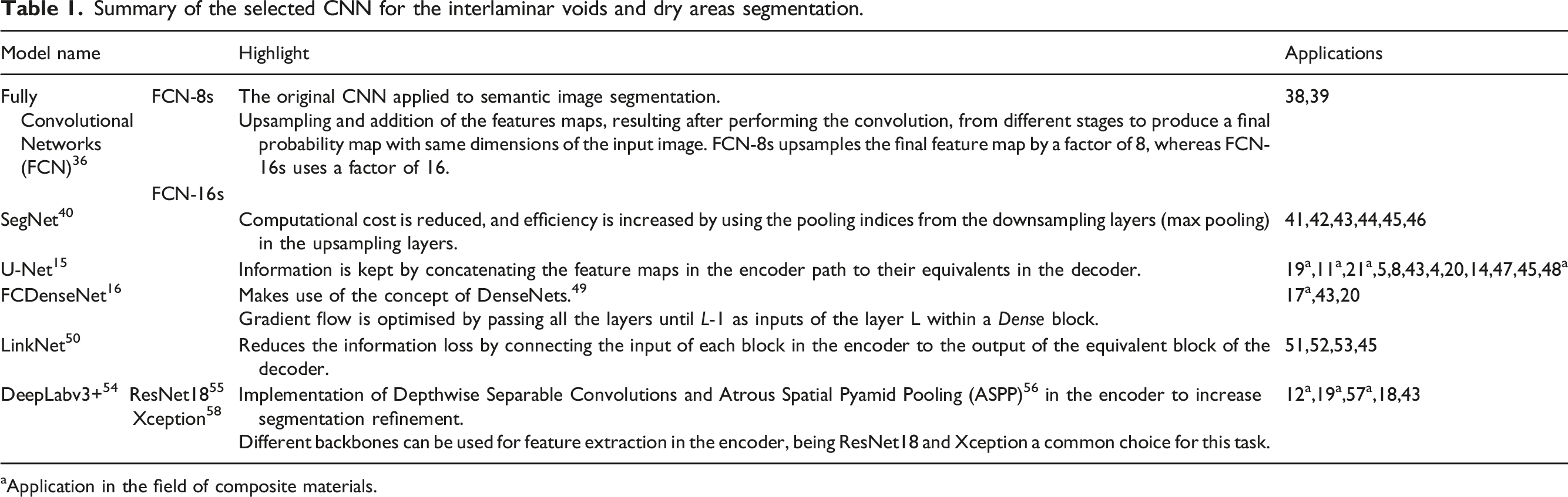
^aApplication in the field of composite materials.

All architectures were implemented in Python 3.6 from scratch using Tensorflow 2.5³⁰ following the instructions indicated at their original publications. Publicly available code was used as inspiration for the implementation of the SegNet,³¹ LinkNet³² and DeepLabv3+ (Xception).³³ Deeplabv3+ (ResNet18) was translated to Python from the Matlab version described in.³⁴ The implementation of the unpooling layer, typical of the SegNet architecture, was obtained from the TensorFlow-Addons package.³⁵ FCN-32s, which is the parent architecture of FCN-16s,³⁶ was initially included in the study, but poor segmentation performance was observed in preliminary trials, therefore it was excluded from the final set of architectures. DeconvNet³⁷ was also considered in preliminary trials, but was omitted here because it is very similar to SegNet.

Training strategy

The image set previously generated in¹³ and consisting of 120 patches with dimensions 128 × 128 pixels was used in this study. The patches were selected from the raw scans of Training Sample 1 and Sample 2. From each scan, an average of 3.77 ± 1.5 patches per slice were manually selected from sixteen slices located the across the full tomogram in a supervised approach, i.e.,, ensuring that a high level of variability in terms of voids and dry areas shapes and sizes were included, in both the slices and patches. This method pursued a three-fold aim: 1) According to,⁵⁹ training a CNN model with patches instead of full-size images was found to provide a better performance since the variability is reduced when using a single patch, compared to using a full-sized slice, which facilitates the learning by the weights of the model. 2) A common training strategy consists of selecting a fixed number of slices from the scan used for training, annotating the full-size slices and then sub-dividing them into smaller patches that are fed to the model.^4,11,20 This strategy was initially considered as it allows for a high volume of training images, but it was rejected due to lengthy annotation time. It is worth noting that manually annotating a single patch took approximately 10 minutes, and therefore annotating a full-size slice would take ∼8 hours (forty-nine patches are contained in a 900 × 900 pixels slice taken from the Training Sample 1 and 2 scans). The strategy proposed in this study sought to optimise the annotation effort. Fifty patches selected across different slices and including a wider typology of features could be annotated within a standard working day of 8h. 3) The slices, from which patches were later extracted, were randomly chosen based on the typology of voids and dry areas they contained, in order to ensure that a high variability was included. This procedure was preferred over selecting slices at specific intervals as it increased the control over the images defining the training set and reduced the risk of oversampling a certain type of feature typology.⁶⁰ A link to access the full set of patches used for training, as well as their location in the scans is provided at the end of the paper.

The associated ground truth masks for the interlaminar voids and dry areas were generated using the Pixel Annotation Tool,⁶¹ and VIA Annotator Software,⁶² respectively. The former software is a semi-automatic method based on the use of an annotation brush and the watershed algorithm to reduce the annotation effort.^63,64 The latter relies on the use of bounding boxes, such as the polygon region shapes used in this study, to annotate the objects of interest in the image. Each greyscale image has three associated binary images, one for each feature, and an additional image for representing the background, i.e., pixels that were not annotated as voids or dry areas. The annotation process took approximately 20 hours. These binary masks contain two types of pixels: white pixels (positive labels) representing the phase of interest (either interlaminar voids or dry areas) and black pixels (negative labels) representing the background.

Three independent training sets consisting of 25, 50, and 100 images were randomly generated from the initial image set. This selection was used to investigate the effect of increasing and decreasing the typical annotation output of a working day (fifty patches) by a factor of two, and therefore allowing the identification of the optimum annotation effort, i.e., obtaining the highest segmentation performance with the lowest annotation time, for the type of images, features and resolution presented in this study. The three sets will be referred to as TS-25, TS-50 and TS-100. In addition, 20 images were selected to act as a control set, i.e., unknown data to the model parameters, therefore allowing the generalisation and evaluation of the model performance during training. The same control set was used across the three training sets to ensure a fair comparison of the training performance. No data augmentation techniques were applied to the training sets. The binary masks generated in ¹³ were used in this study after implementing minor improvements in two of the ground truths images to avoid the multiclass case in which a pixel is assigned to more than one category during the annotation process. Details about the changes are provided in the supplementary information (Appendix A).

During training the models learn to segment the features of interest following an iterative process. In each iteration, also called an epoch, the models are fed the training set in batches of N images together with the associated binary masks. Therefore, M/B steps are needed to complete an epoch, where M is the size of the training set and B is the batch size. For each greyscale image, the models receive three binary masks: one for each phase, i.e., interlaminar voids and dry areas, and an additional mask for the background, representing the pixels not belonging to either of the previous classes. At the end of each step within the epoch, the model generates a probability map for each greyscale image contained in the batch via the Softmax function, where each pixel contains the probability of belonging to each class. These probability maps are compared to the ground truth masks and generate an error, which is measured through the Categorical Cross-Entropy Loss function (1) in this study. The loss is backpropagated through the network and the trainable parameters, also called weights, are updated with the aim of reducing the loss in the following step.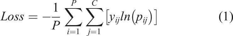

L o s s = - \frac{1}{P} \sum_{i = 1}^{P} \sum_{j = 1}^{C} [y_{i j} \ln (p_{i j})]

(1)

Where

P

is the total number of pixels in each batch of images, C is the number of categories (background, interlaminar void and dry area) and

y_{i j}

and

p_{i j}

stand for the ground truth value and the predicted probability of the pixel i of belonging to the class j.

CNN hyperparameters selection

Optimising CNN performance requires selecting a set of user-defined variables, also known as hyperparameters. These non-trainable variables define the architecture properties, such as the number and typology of the layers integrating the network, and the training and inference process. Tuning the values of the hyperparameters to achieve an optimum performance of the models is a costly activity from a computing effort and time standpoint.^10,20 In this study, a set of the most relevant hyperparameters was optimised using a grid-search approach, consisting of the evaluation of all possible combinations of the selected hyperparameters values. The following set of hyperparameters was chosen due to their reported contribution to the model performance:

• Learning rate (LR): This hyperparameter defines the amount by which the model weights are updated during backpropagation and control the speed of the learning process; it is recognised as one of the hyperparameters having the greatest impact on the model performance.^3,65 Considering the recommendations in the literature ^3,66,67 and the range of values used in the studies presented in Table 1, three learning rates were evaluated: 10⁻², 10⁻³, and 10⁻⁴.

• Learning rate reduction factor: As the training progresses, the model may benefit from reducing the learning rate in order to find further optimal states that would have been overlooked by larger learning rates.¹⁹ To account for this observation, the learning rate was automatically reduced by a user-defined factor if the control set loss did not improve during five consecutive epochs. Two reduction factors, previously reported in the literature,^8,13 were studied: 0.5 and 0.9.

• Optimiser: It defines the algorithm used for updating the network weights during training. Two optimisation algorithms were evaluated: Stochastic Gradient Descent (SGD) ⁶⁸ and ADAM.⁶⁷ SGD was developed as an improvement of a previous gradient-based optimisation algorithm called “Vanilla” by computing the gradient in just a selection of samples, hence the term stochastic, reducing the computing complexity. In 2015, ADAM was proposed as a more efficient implementation of stochastic gradient-based algorithms by incorporating adaptative learning rates of different parameters, and combining the virtues of other optimisers such as AdaGrad ⁶⁹ and RMSProp.⁷⁰ SGD and ADAM are frequently regarded as two of the most popular state-of the-art methods³ and are widely used in the studies included in Table 1.

• Batch normalisation: This technique was introduced by Ioffe et al. ⁷¹ and consists of the normalisation of the output of the layer L before being fed to the layer L + 1. It has been claimed to reduce the training effort as well as minimising the risk of overfitting, which appears when the model fails to generalise in unknown data despite achieving a high performance in the training set.^21,71 Two options were considered regarding the batch normalisation layers, whether they were included in the architecture (True) or not (False).

The rest of the hyperparameters were kept constant during model training. The maximum number of epochs was set to 300, and an early-stopper callback that would stop the model training if the control set loss did not improve for 30 consecutive epochs, further minimising the training time. This value represents the 10% of the maximum number of epochs and it is consistent with the values reported in previous studies.^43,47,72 The batch size was one, as reported in previous studies,^11,13,19 allowing the maximisation of the frequency at which the weights are updated during each epoch. The combination of hyperparameters values and the model state (weight values) at the epoch minimising the control set loss was saved (Table 2) and used for a further segmentation of voids and dry areas in the Validation Sample scan.

Table 2.

Final hyperparameter selection and elapsed training and prediction times.

CNN	Training set	Batch norm.	Learning rate (LR)	LR reduction factor	Output stride	Training epochs	Number of parameters	Training time (min.)	Prediction time (min.)
FCDenseNet	25	Yes	10^–2	0.9	NA^a	66	9,422,243	6.56	76.9
	50	No	10^–3	0.9	NA	47	9,216,099	5.01	69.0
	100	No	10^–3	0.5	NA	58	9,216,099	10.14	67.6
FCN-16s	25	Yes	10^–3	0.9	NA	50	134,332,252	8.57	54.8
	50	Yes	10^–3	0.9	NA	49	134,332,252	9.94	55.0
	100	No	10^–3	0.9	NA	47	134,282,588	12.25	53.2
FCN-8s	25	Yes	10^–3	0.9	NA	52	134,326,258	9.24	56.5
	50	No	10^–3	0.5	NA	54	134,276,594	10.81	53.9
	100	Yes	10^–2	0.5	NA	45	134,326,258	14.20	55.2
LinkNet	25	No	10^–3	0.9	NA	55	11,521,443	2.13	52.6
	50	No	10^–3	0.5	NA	44	11,521,443	2.03	52.5
	100	No	10^–3	0.9	NA	49	11,521,443	3.85	52.6
ResNet18	25	No	10^–3	0.5	8	52	16,590,387	2.25	55.8
	50	No	10^–3	0.5	8	51	16,590,387	2.92	53.6
	100	No	10^–3	0.5	8	62	16,590,387	5.33	56.0
SegNet	25	Yes	10^–2	0.5	NA	45	29,495,107	2.75	65.0
	50	Yes	10^–3	0.9	NA	50	29,495,107	4.13	64.3
	100	Yes	10^–3	0.9	NA	48	29,495,107	5.81	61.6
U-Net	25	Yes	10^–3	0.9	NA	54	31,058,115	3.20	58.8
	50	No	10^–3	0.9	NA	68	31,030,723	4.66	58.5
	100	No	10^–3	0.5	NA	55	31,030,723	5.25	58.7
Xception	25	No	10^–3	0.9	8	86	40,948,811	8.77	76.0
	50	No	10^–3	0.9	16	71	40,948,811	8.37	68.3
	100	No	10^–3	0.5	8	79	40,948,811	16.89	72.0

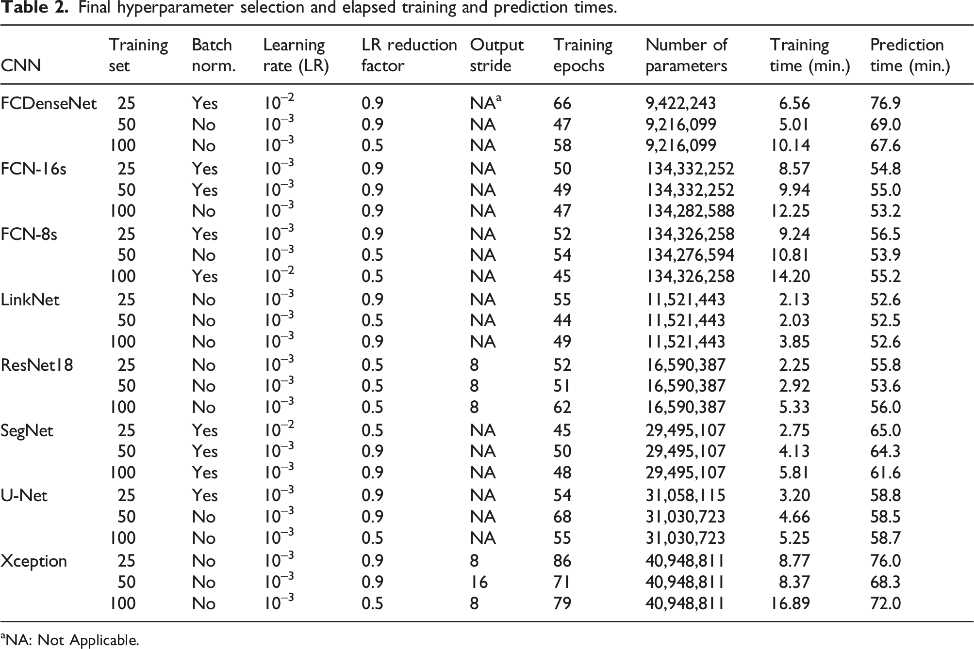
^aNA: Not Applicable.

For each architecture 72 models were generated (2 optimisers × 3 LRs × 2 LR reduction factors × 2 batch normalisation × 3 training sets), with 72 additional models for each DeepLabv3 + architecture to account for the output stride, which controls the ratio between the shapes of the input image and the output of the feature extractor. Following the recommendations proposed in the original paper,⁵⁴ the output stride was set to either 8 or 16. In total, 720 models were evaluated over 115 hours in a GPU Nvidia RTX 3080. It is worth noting that certain hyperparameter combinations resulted in the non convergence (NC) of 165 models. This effect was frequent in both Deeplabv3+ (Xception: 73 NCs, ResNet18: 84 NCs) architectures, particularly when the batch normalisation layer was included in the architecture.

The U-Net models presented in this study differed from those included in ¹³ in the following aspects: 1) Correction of mislabelled pixels contained in the training set, 2) Training has been carried out in a GPU, as opposed of the CPU-based training used in the previous study, 3) A hyperparameter optimisation step has been included in the present analysis. Due to the aforementioned changes, the performance results included here may differ from the ones discussed in.¹³

Following the training, the models are used to generate the probability maps corresponding to the interlaminar void and dry area phases in the Validation Sample scan containing a thousand 2D-slices of 700 × 700 pixels. Detailed information about the strategy followed to obtain the phase predictions in a scan whose dimensions exceed the dimensions of the images used in the training of the deep learning models can be found in.¹³ The 3D probability maps for each phase are subsequently converted to binary 3D images upon the application of a cut-off probability (p_t). If the corresponding greyscale pixel receives a probability equal to or greater than p_t belonging to the phase of interest, the pixel is assigned a value of 255 in the binary 3D image, and a value of 0 if the probability is below p_t. For each model, the combination of both cut-off probabilities (interlaminar voids and dry areas) was calculated so that the average segmentation performance (MCC), considering each phase and ROI was maximised. Additional information describing the methodology followed for the selection of the cut-off probabilities as well as the detailed list of final cut-off probabilities for each phase and model is included in the supplementary information (Appendix B).

Finally, the plugin BoneJ ⁷³ is used for the characterisation of the phases. Average values are expressed as mean ± standard deviation (µ ± σ). The complete flowchart regarding the model training and scan segmentation is provided in Figure 1.

Figure 1.

Deep Learning segmentation flowchart. Following the generation of the CT micrographs for the three samples (a), an image set is created after randomly selecting and manually annotating 120 patches from the scans of Training Sample 1 and 2 (b). This image set is subsequently split into two categories: training set, with three different sizes, and control set (c). These two sets are used for the training of eight CNN architectures, involving an hyperparameters optimisation step (d). After training, the models segment the interlaminar voids and dry areas in the Validation Sample allowing the phase characterisation and the assessment of the models performance in the selected ROIs, whose exact location was described in ¹³ (e).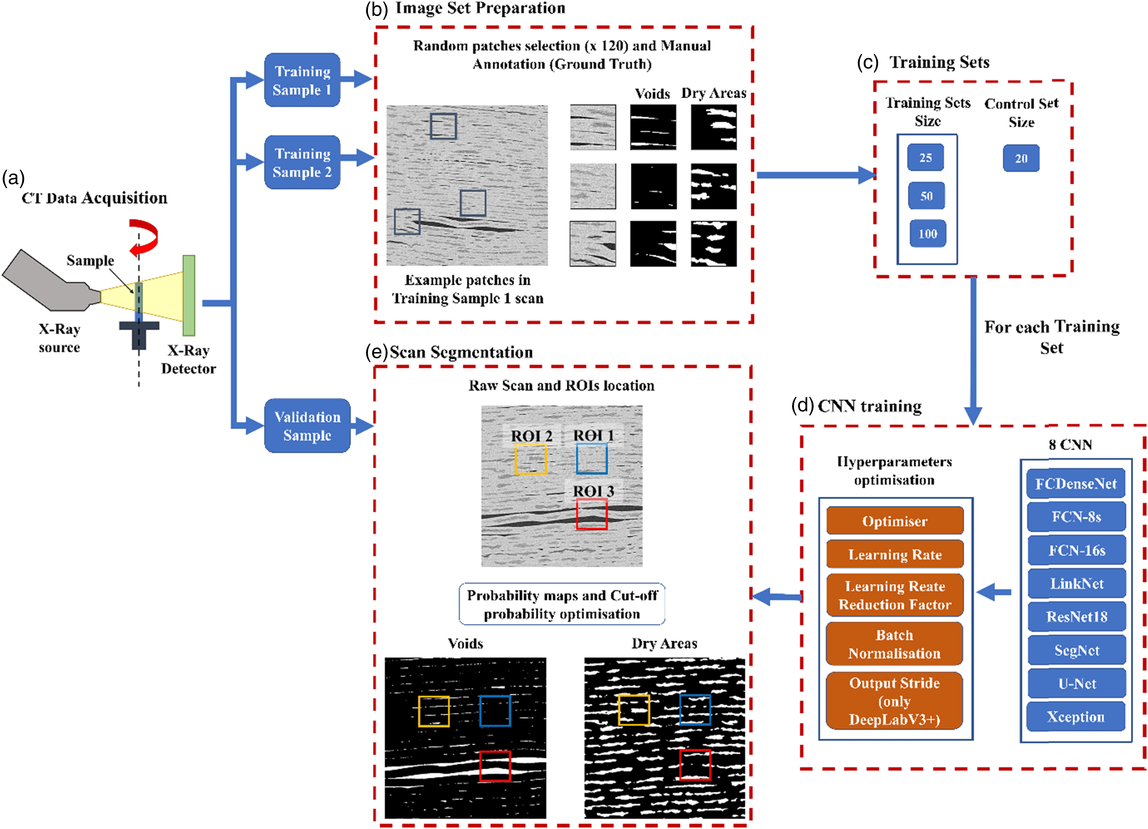

Performance evaluation

Three regions of interest (ROI) having twenty 2D consecutive slices of 128 × 128 pixels and located in its central volume, slices 491–510, were selected at different locations and containing different levels of interlaminar porosity after visual assessment (Figure 1). The ROI locations and dimensions are the same as used in.¹³ This selection will provide information about the ability of the different models and training set sizes to segment different levels of porosity. The ground truth masks of the ROIs representing the interlaminar voids and dry areas were manually generated in a previous study ¹³ in the same fashion as the training and control set ground truths. The same ROIs were then selected in the segmented scan provided by the eight models trained with each of the training set sizes. The interlaminar voids and dry areas ground truth masks are compared to their segmented counterparts, and each pixel is assigned a category depending on the correctness of the prediction: positively labelled and positively predicted (True Positive or TP), positively labelled but negatively predicted (False Negative or FN), negatively labelled and negatively predicted (True Negative or TN) or negatively labelled but positively predicted (False Positive or FP). These four categories within each of the binary masks, allow the definition of the following segmentation performance metrics: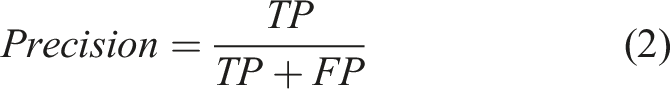

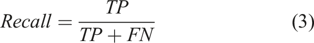
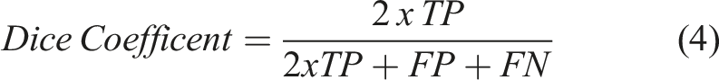
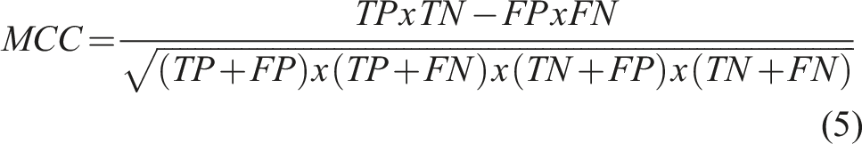
P r e c i s i o n = \frac{T P}{T P + F P}

(2)

R e c a l l = \frac{T P}{T P + F N}

(3)

D i c e C o e f f i c e n t = \frac{2 x T P}{2 x T P + F P + F N}

(4)

M C C = \frac{T P x T N - F P x F N}{\sqrt{(T P + F P) x (T P + F N) x (T N + F P) x (T N + F N)}}

(5)

Precision (Equation (2)) informs about the level of noise (false positives) present in the prediction, whereas recall (Equation (3)) provides information about the ability of the model to capture the true labels existing in the ground truth. The Dice Coefficient (Equation (4)), also called F1-Score, ^74,75 and the Matthews Correlation Coefficient (MCC) (Equation (5)) ⁷⁶ integrate the four categories into one formula and provide and overall indicator of the segmentation performance for each phase provided by each of the models.

Precision, Recall, and Dice Coefficient are defined in the interval [0, 1], where a value closer to 1 meaning better performance compared to the ground truth. The MCC is defined in the interval [-1, 1], where a value closer to −1 indicates a poor segmentation performance, 0 means that the segmentation provided by the model is not better than a random segmentation, and 1 is a perfect correlation between the model segmentation and the ground truth mask.

Results

Network training and prediction

The overall aim for model training is to achieve the minimum control set loss in the shortest time, indicating a fast convergence to the optimum state of the weights for each model. The combination of the hyperparameter values minimising the control set loss is presented in Table 2. All models benefited from the use of ADAM as the optimisation algorithm. Additionally, an initial learning rate of 10⁻³ was the preferred option in 87% of models, whereas none of the models benefitted from a reduction of an order of magnitude in the initial value in the learning rate. The batch normalisation layer was found in nine models. LinkNet, ResNet18, and Xception minimised their respective control set loss without featuring such layers when trained with any of the three training set sizes. An output stride = 8 showed an improvement in performance during training for all DeepLabv3 + models, except for the Xception architecture trained with 50 images.

The total number of parameters notably differed from one architecture to other due to the differences in number and size of convolutional layers. FCDenseNet models accounted for just 9 million parameters, whereas FCN-8s and FCN-16s contained 134 million.

According to Figure 2, increasing the training set size has a positive effect on reducing the control set loss for all architectures. U-Net was found to provide the lowest control set loss regardless of the training set size, reaching a minimum of 0.13 when trained with 100 images. The highest control set loss was found in the three models featuring the FCN-16s architecture (TS-25: 0.3, TS-50: 0.26, TS-100: 0.23). SegNet most benefited from increasing the training set size from 25 to 50, with a decrease of 26% of the control set loss, whereas FCN-16s had a reduction of 12% in the control set loss when increasing from 50 to 100 training images. It is worth noting that the reduction in the control set loss is more acute after doubling the initial 25 training images to 50, than when doubling from 50 to 100 images (−13.25 ± 5.48% vs. −8.97 ± 2.85%). Training time generally increased with training set size. LinkNet models converged the fastest to their respective minimum control loss, due to a light and simple architecture. In contrast, heavier architectures (FCN-8s, FCN-16s) and denser architectures (DeepLabv3+ (Xception) and FCDenseNet) took between 2–6 times longer to reach their optimum state. All models converged to the optimal state before reaching 100 epochs and their control set loss increased after passing this point, thus confirming the suitability of the user-defined 300 epochs limit during training. A similar trend was observed during the prediction step. The DeepLabv3+ (Xception) models took on average 72.1 ± 3.89 minutes to generate the full set of probability maps, a 37% increase with respect to the fastest model (LinkNet: 52.56 ± 0.07 minutes).

Figure 2.

Training and prediction time for each CNN and training set size.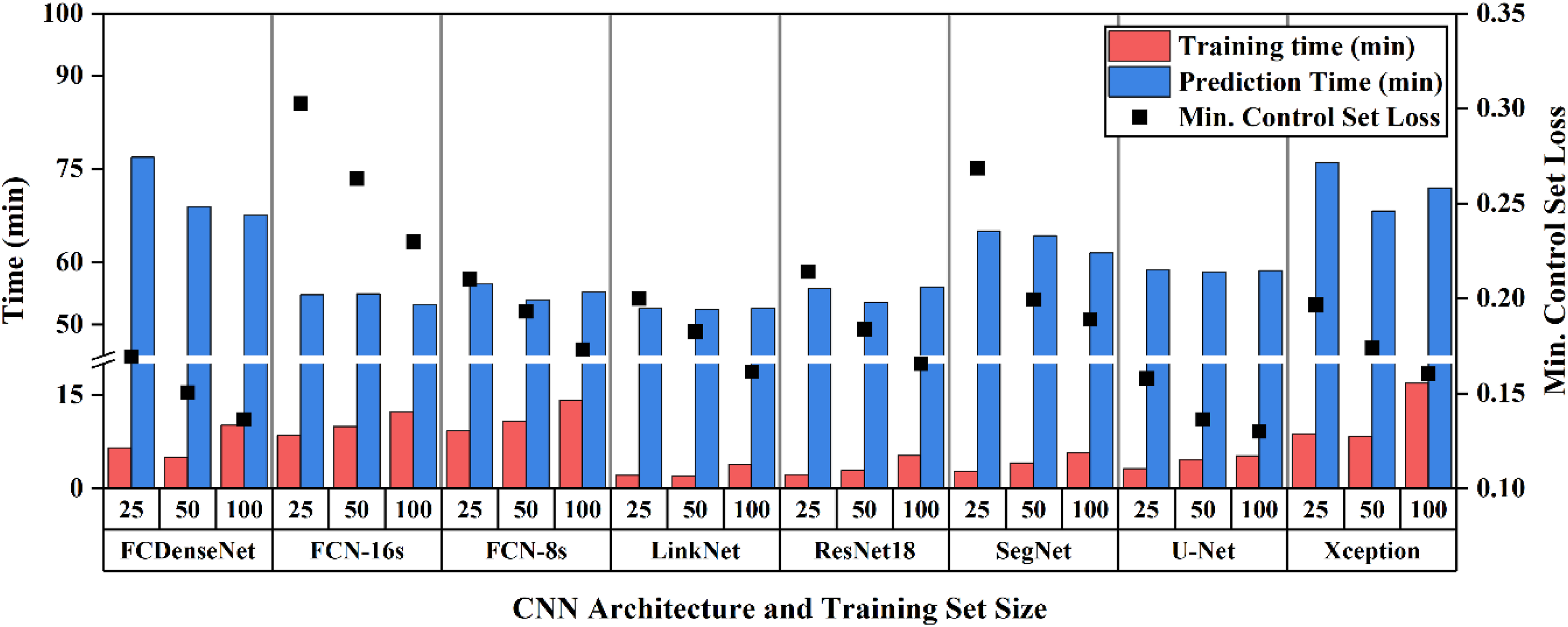

Entire scan segmentation

Figure 3 compares and contrasts the most and least suitable models to segment the interlaminar voids or dry areas. It can be observed that initially some dry areas, which contain dark pixels due to a high content of air, are initially either misclassified or completely missed by the two networks. However, as the training set increases, U-Net achieves a perfect classification and FCN-16s also increases their detectability. From visual assessment, U-Net provides the highest accuracy in the segmentation of both interlaminar voids and dry areas, regardless of the training set size.

Figure 3.

Segmentation of interlaminar voids (blue) and dry areas (red) of a full-sized slice located at the centre of the entire scan, after training with 25 and 100 images, for the best performing network (U-Net) and the networks providing the lowest MCC score for voids and dry areas (FCN-16s). The black arrow points at a dry area displaying a grey intensity characteristic of the interlaminar voids and its segmentation by the different models.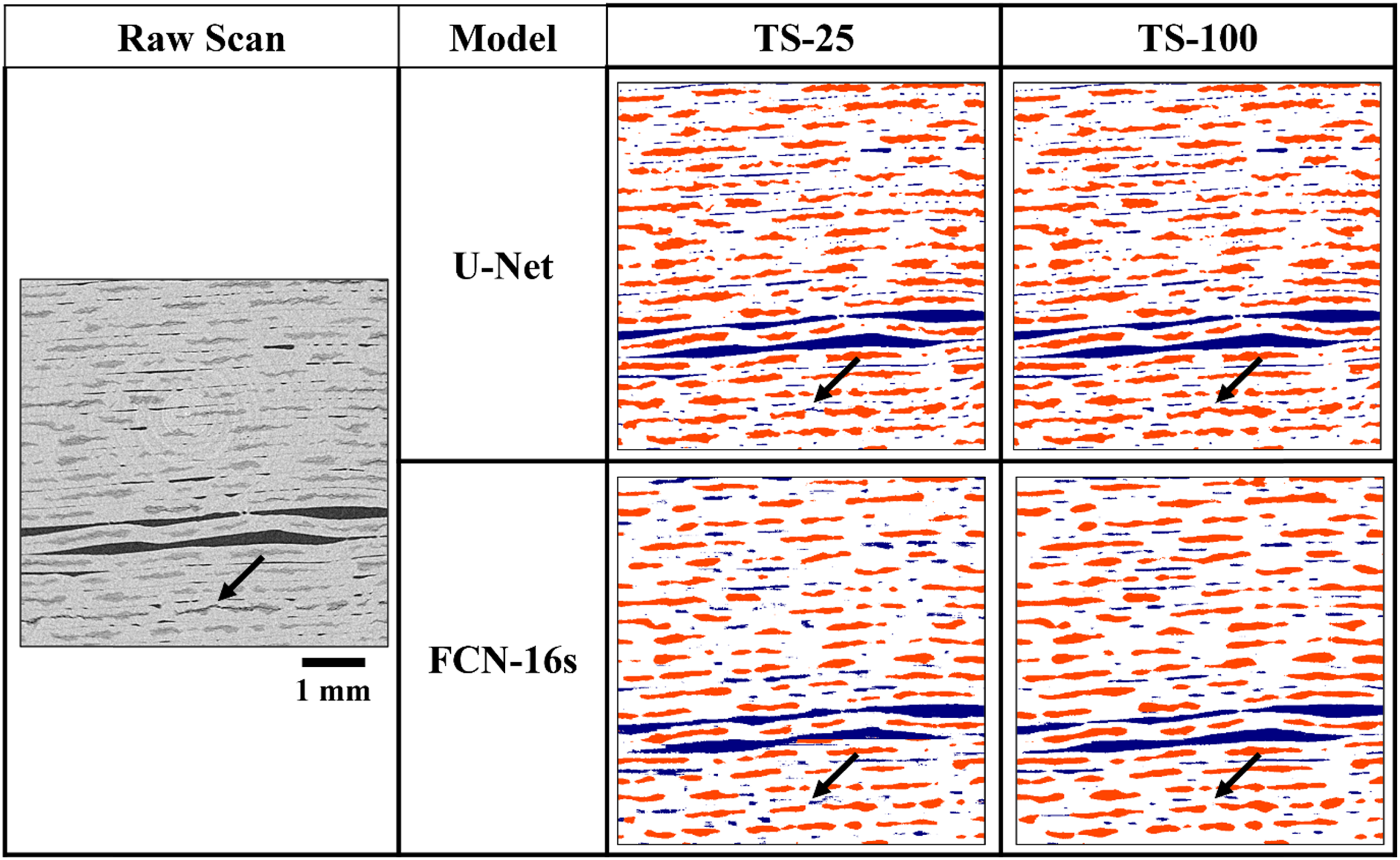

From a quantitative standpoint, it has been observed that increasing the training set size impacts the distribution of the interlaminar voids and dry areas (Figure 4). On the one hand, the computed average porosity is comparable across the three training set sizes (TS-25:5.75 ± 0.4%, TS-50: 5.51± 0.16%, TS-100: 5.61 ± 0.2%), but the dispersion in the average interlaminar void volume and individual void counts were notably reduced after a four-fold increase of the training set size (TS-25: 8.07 × 10⁵ ± 5.42 × 10⁵ µm³/void and 2.75 × 10⁴ ± 1.84 × 10⁴ counts, TS-100: 8.39 × 10⁵ ± 1.86 × 10⁵ µm³/void and 1.92× 10⁴ ± 4.72 × 10³ counts). ResNet18 segments the large voids effectively, but misses the smaller voids when compared to the average void count of the models trained with twenty-five and fifty images. On the other hand, FCN-16s captures a higher portion of smaller voids. The behaviour observed in the segmentation produced by FCN-16s implies that this model captures less noise as the training set size increases, which is usually characterised by small but numerous conglomerates of mislabelled pixels that lower the average volume and increase the counts. The segmentation provided by both architectures converge to the values obtained by the other networks when a larger training set is used.

Figure 4.

Quantitative assessment regarding the segmentation of the interlaminar voids and dry ares provided by each network for each training set size (25, 50 and 100).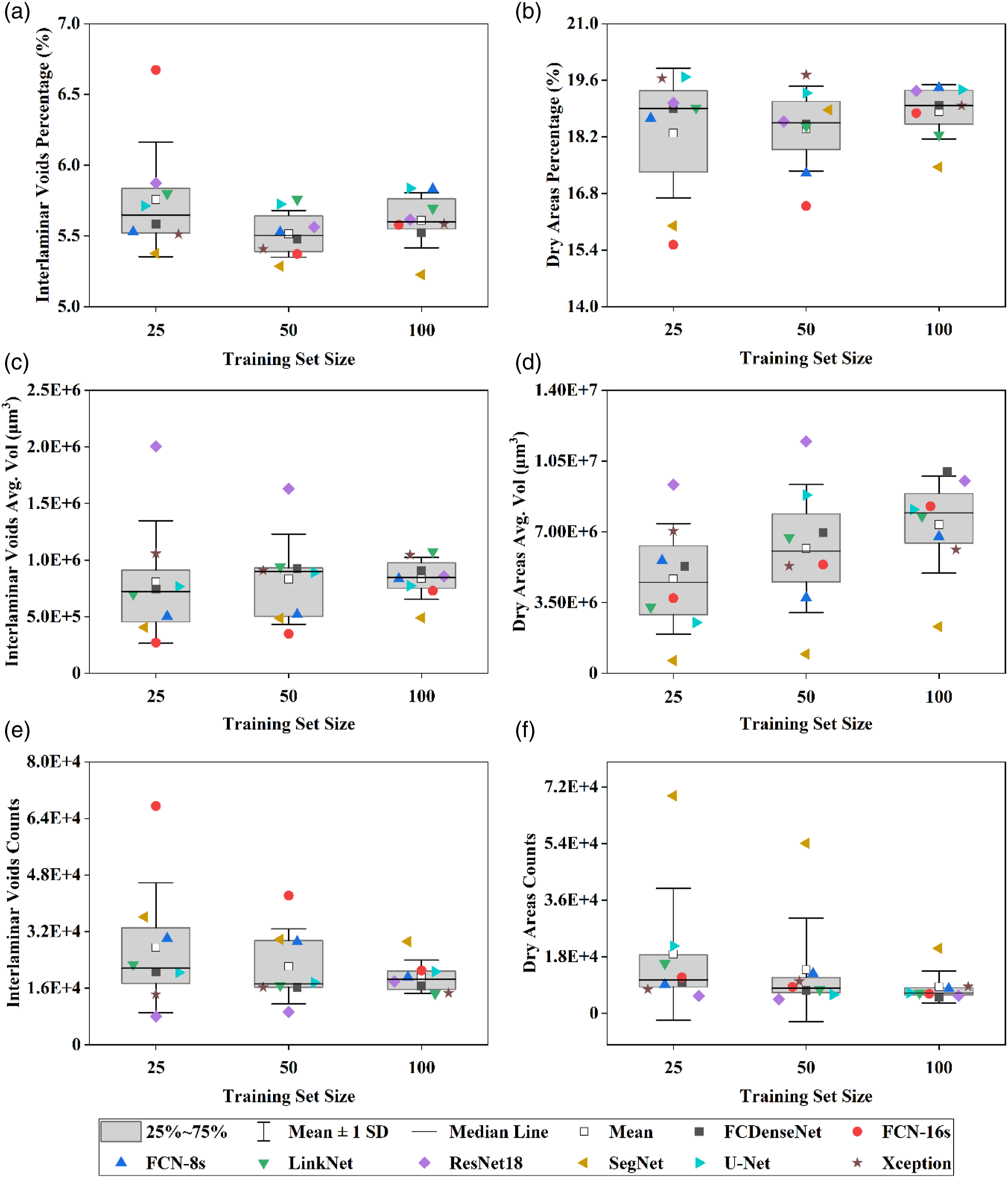

The average dry areas percentage remains approximately constant but also accounts for a reduction of the dispersion (TS-25:18.29 ± 1.61%, TS-50: 18.4 ± 1.05%, TS-100: 18.82 ± 0.67%), along with an increase of the average dry area volume and a decrease of the dry area counts as the training set size increases as the segmentation noise and mislabelling is reduced. The segmentation of dry areas produced by the ResNet18 produces the same effect as previously described in the segmentation of interlaminar voids since this architecture segments the largest dry area but accounting for the lowest counts when trained with twenty-five and fifty images. On the other hand, SegNet provides the lowest dry area average volume across the three training set sizes, due to the high number of dry area counts for a comparable porosity estimation to the rest of the models.

Performance evaluation

Voids

ROI 1

The biggest difference in performance between the Deep Learning models was observed in ROI 1, which has a ground truth porosity of 1.07% and features small-sized interlaminar voids characteristic of aerospace quality parts after manufacture. The model performance results are contained in Table 3. Of the models considered here, FCDenseNet exhibits the best performance when trained with just 25 images, achieving an MCC and Dice coefficient of 0.87. U-Net provided the second highest MCC and Dice scores (0.86) using the smallest training set of 25 and the best performance when the training set was doubled to 50 and then doubled again to 100. Increasing the training set size resulted in an improvement of the recall value (TS-25: 0.82, TS-50: 0.84, TS-100: 0.86) as a higher portion of positive labels present in the ground truth are captured in the U-Net prediction. Precision reaches the maximum for TS-50, and then decreases after using 100 training images (TS-25: 0.90, TS-50: 0.95, TS-100: 0.92). FCDenseNet consistently provides the highest precision score (0.98) and showcases the ability of the model to capture not only low noise, but also small voids annotated in the ground truth. FCN-16s shows the poorest segmentation performance, with a decrease of 63% in the MCC score with respect to FCDenseNet when trained with 25 images. Increasing the size of the training set to 100 images allows FCN-16s to achieve an MCC score of 0.61, which is 31% lower than score provided by U-Net.

Table 3.

Interlaminar voids segmentation results for ROI 1.

ROI id	Model	Training set size	Porosity (%)	Precision	Recall	Dice	MCC
1	FCDenseNet	25	0.86	0.98	0.78	0.87	0.87
		50	0.82	0.98	0.75	0.85	0.86
		100	0.85	0.98	0.78	0.87	0.87
	FCN-16s	25	0.72	0.40	0.27	0.32	0.32
		50	0.49	0.54	0.25	0.34	0.36
		100	1.30	0.56	0.68	0.61	0.61
	FCN-8s	25	1.14	0.67	0.72	0.69	0.69
		50	1.09	0.65	0.66	0.65	0.65
		100	0.97	0.77	0.71	0.74	0.74
	LinkNet	25	1.10	0.75	0.77	0.76	0.76
		50	0.97	0.86	0.78	0.82	0.82
		100	0.94	0.89	0.78	0.83	0.83
	ResNet18	25	1.01	0.79	0.74	0.77	0.76
		50	0.95	0.87	0.78	0.82	0.82
		100	1.12	0.77	0.81	0.79	0.79
	SegNet	25	0.49	0.56	0.26	0.35	0.38
		50	0.88	0.81	0.67	0.73	0.73
		100	1.10	0.62	0.64	0.63	0.63
	U-Net	25	0.98	0.90	0.82	0.86	0.86
		50	0.95	0.95	0.84	0.89	0.90
		100	1.00	0.92	0.86	0.89	0.89
	Xception	25	0.99	0.79	0.73	0.76	0.76
		50	1.14	0.77	0.82	0.80	0.80
		100	1.15	0.76	0.81	0.78	0.78

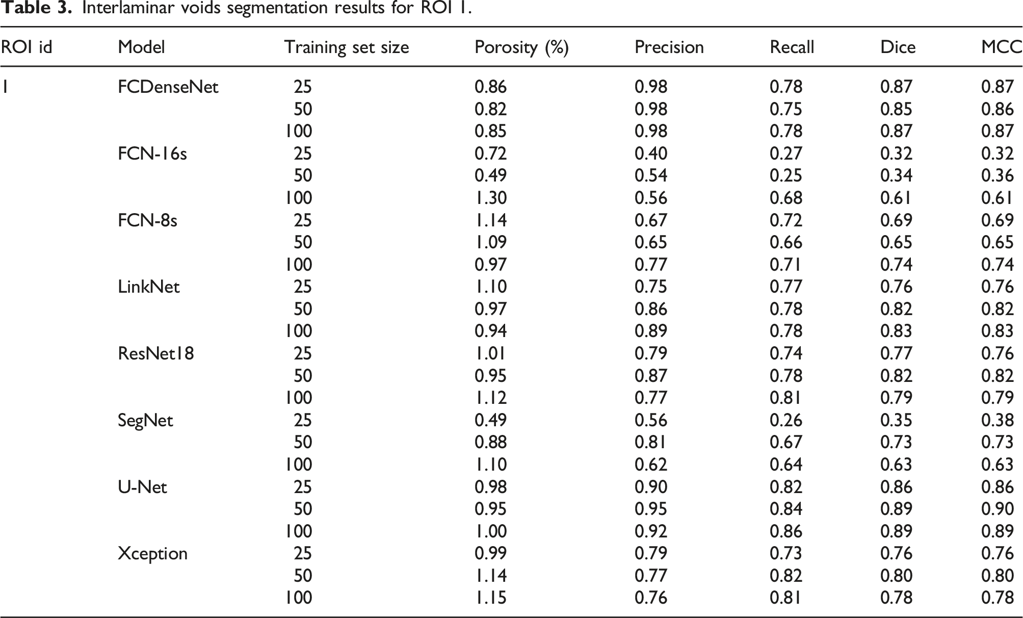
Regarding the porosity estimation, FCN-16s provides the highest porosity estimation (1.3%) after training with 100 images. However, this value does not imply a high segmentation performance. On the contrary, it comes at the expense of a low precision (0.56) and relatively high recall (0.68), meaning that a high portion of false positives and a low number of false negatives are captured. FCN-16s (TS-50) and SegNet (TS-25) account for the lowest porosity estimation (0.49), mainly driven by the fact that both models also provide the lowest recall (0.25 and 0.26). These two models also exhibit the biggest increase in their recall value after doubling the size of the training set (172% and 159% improvement).

ROI 2

This sub-volume accounts for a ground truth interlaminar porosity of 6.09% and contains medium-sized interlaminar voids that occur after lay-up of composite materials. In this ROI, the difference between the highest and lower performer is reduced (Table 4). FCN-16s achieves the lowest MCC for each of the training sets (TS-25: 0.50, TS-50: 0.6, TS-100: 0.69), whereas U-Net and FCDenseNet provide the best performance regardless of the training set size, with almost identical Dice and MCC values, both metrics above 0.93.

Table 4.

Interlaminar voids segmentation results for ROI 2.

ROI id	Model	Training set size	Porosity (%)	Precision	Recall	Dice	MCC
2	FCDenseNet	25	6.20	0.93	0.95	0.94	0.93
		50	5.84	0.96	0.92	0.94	0.94
		100	5.93	0.96	0.93	0.94	0.94
	FCN-16s	25	7.23	0.49	0.58	0.53	0.50
		50	4.45	0.73	0.53	0.61	0.60
		100	6.80	0.67	0.75	0.71	0.69
	FCN-8s	25	5.17	0.85	0.72	0.78	0.77
		50	5.96	0.87	0.85	0.86	0.85
		100	6.33	0.87	0.91	0.89	0.88
	LinkNet	25	6.14	0.87	0.88	0.88	0.87
		50	6.25	0.88	0.90	0.89	0.88
		100	6.03	0.91	0.90	0.91	0.90
	ResNet18	25	6.62	0.82	0.89	0.86	0.85
		50	5.86	0.89	0.85	0.87	0.86
		100	6.04	0.89	0.88	0.89	0.88
	SegNet	25	4.67	0.93	0.72	0.81	0.81
		50	5.76	0.93	0.88	0.91	0.90
		100	5.20	0.97	0.83	0.89	0.89
	U-Net	25	5.95	0.94	0.92	0.93	0.93
		50	6.23	0.93	0.95	0.94	0.94
		100	6.19	0.93	0.95	0.94	0.94
	Xception	25	5.82	0.89	0.85	0.87	0.86
		50	5.77	0.92	0.88	0.90	0.89
		100	5.93	0.92	0.90	0.91	0.90

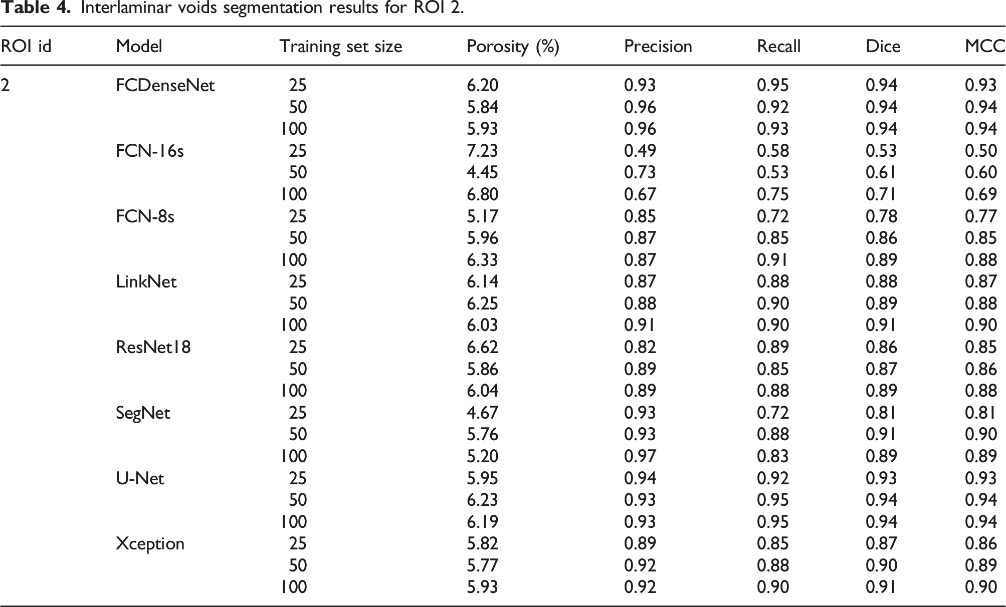
The biggest deviation with respect to the ground truth interlaminar porosity is provided by FCN-16s when trained with 50 images (4.45%) as it accounts for the lowest recall (0.53), which implies a low number of true positives and a relatively high precision (0.73). LinkNet (TS-25) and ResNet18 (TS-100), on the other hand, provide the smallest deviation with respect to the ground truth porosity. This is a consequence of registering a similar level of false positives and false negatives, which cancels out when computing the sub-volume porosity.

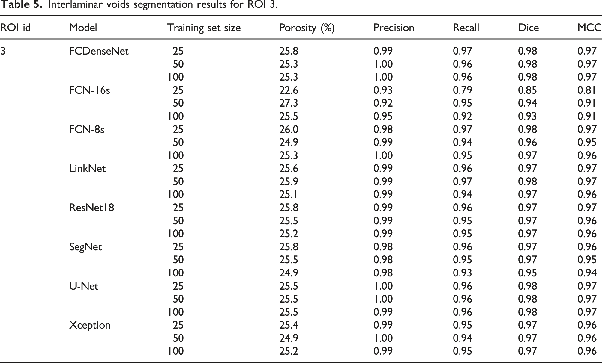
ROI 3

This region contains large voids and high ground truth interlaminar porosity (26.4%) characteristic of defects that would result in part rejection due to poor quality. FCDenseNet and U-Net provide the highest segmentation performance with identical MCC (0.97) and Dice (0.98) across the three training set sizes (Table 5), whereas FCN-16s register the lowest segmentation scores (Dice > 0.85, MCC > 0.81). The rest of models provide a consistently high precision (>0.98), recall (0.93), Dice (0.95) and MCC (0.94), regardless of the image set size used for training.

Table 5.

Interlaminar voids segmentation results for ROI 3.

ROI id	Model	Training set size	Porosity (%)	Precision	Recall	Dice	MCC
3	FCDenseNet	25	25.8	0.99	0.97	0.98	0.97
		50	25.3	1.00	0.96	0.98	0.97
		100	25.3	1.00	0.96	0.98	0.97
	FCN-16s	25	22.6	0.93	0.79	0.85	0.81
		50	27.3	0.92	0.95	0.94	0.91
		100	25.5	0.95	0.92	0.93	0.91
	FCN-8s	25	26.0	0.98	0.97	0.98	0.97
		50	24.9	0.99	0.94	0.96	0.95
		100	25.3	1.00	0.95	0.97	0.96
	LinkNet	25	25.6	0.99	0.96	0.97	0.97
		50	25.9	0.99	0.97	0.98	0.97
		100	25.1	0.99	0.94	0.97	0.96
	ResNet18	25	25.8	0.99	0.96	0.97	0.97
		50	25.5	0.99	0.95	0.97	0.96
		100	25.2	0.99	0.95	0.97	0.96
	SegNet	25	25.8	0.98	0.96	0.97	0.96
		50	25.5	0.98	0.95	0.97	0.95
		100	24.9	0.98	0.93	0.95	0.94
	U-Net	25	25.5	1.00	0.96	0.98	0.97
		50	25.5	1.00	0.96	0.98	0.97
		100	25.5	0.99	0.96	0.98	0.97
	Xception	25	25.4	0.99	0.95	0.97	0.96
		50	24.9	1.00	0.94	0.97	0.96
		100	25.2	0.99	0.95	0.97	0.96

Dry areas

Since the three ROIs contain an equivalent level of dry areas (18.9 ± 1.6%), the segmentation performance values have been averaged across the three ROIs and summarised in Table 6. All architectures achieve a high MCC (>0.74) and Dice (>0.78) for the three image sets. Furthermore, the average Dice and MCC improve as the training set size increases for all architectures, except FCN-8s and SegNet. FCDenseNet and U-Net consistently provide the highest segmentation performance (MCC > 0.88, Dice > 0.9). The models featuring FCDenseNet architecture captured the lowest number of false positive labels on average (Precision > 0.94), while the U-Net models retrieve the highest portion of ground truth data (Recall > 0.88). FCN-16 computes the lowest MCC and Dice among all architectures and training set sizes, but it also sees the highest relative increase (7.5%) in the segmentation performance when passing from 50 to 100 training images (MCC (TS-50): 0.76 vs MCC (TS-100): 0.81), mainly due to an improvement of the recall value (TS-50: 0.7 vs TS-100: 0.82). This improvement translated into a significant reduction of the deviation between the average dry areas percentage calculated for each FCN-16s model (TS-25: 14.3 ± 0.9%, TS-50: 14.8 ± 0.9, and TS-100: 17.8 ± 0.9%) and the ground truth value.

Table 6.

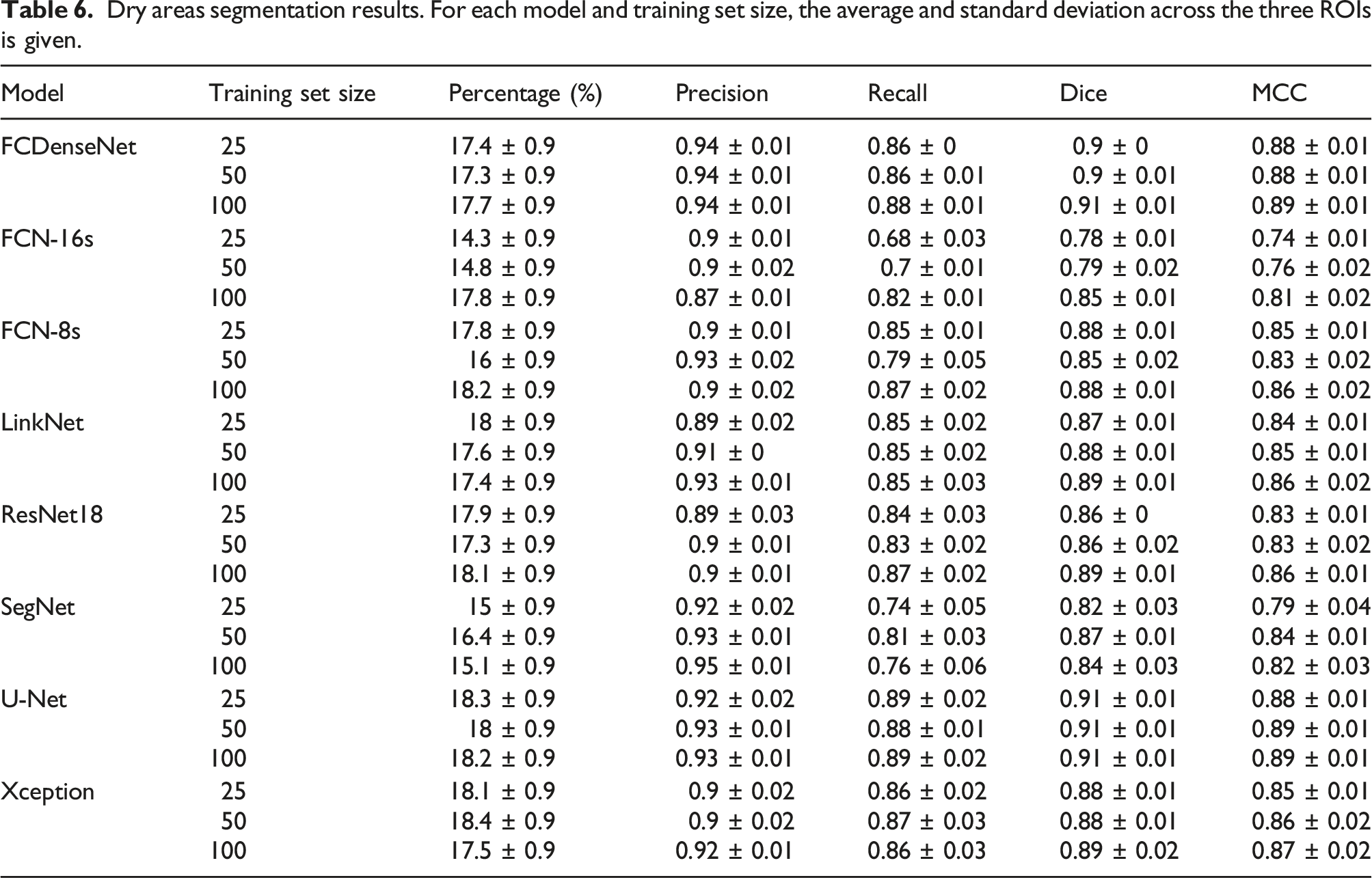
Dry areas segmentation results. For each model and training set size, the average and standard deviation across the three ROIs is given.

Model	Training set size	Percentage (%)	Precision	Recall	Dice	MCC
FCDenseNet	25	17.4 ± 0.9	0.94 ± 0.01	0.86 ± 0	0.9 ± 0	0.88 ± 0.01
	50	17.3 ± 0.9	0.94 ± 0.01	0.86 ± 0.01	0.9 ± 0.01	0.88 ± 0.01
	100	17.7 ± 0.9	0.94 ± 0.01	0.88 ± 0.01	0.91 ± 0.01	0.89 ± 0.01
FCN-16s	25	14.3 ± 0.9	0.9 ± 0.01	0.68 ± 0.03	0.78 ± 0.01	0.74 ± 0.01
	50	14.8 ± 0.9	0.9 ± 0.02	0.7 ± 0.01	0.79 ± 0.02	0.76 ± 0.02
	100	17.8 ± 0.9	0.87 ± 0.01	0.82 ± 0.01	0.85 ± 0.01	0.81 ± 0.02
FCN-8s	25	17.8 ± 0.9	0.9 ± 0.01	0.85 ± 0.01	0.88 ± 0.01	0.85 ± 0.01
	50	16 ± 0.9	0.93 ± 0.02	0.79 ± 0.05	0.85 ± 0.02	0.83 ± 0.02
	100	18.2 ± 0.9	0.9 ± 0.02	0.87 ± 0.02	0.88 ± 0.01	0.86 ± 0.02
LinkNet	25	18 ± 0.9	0.89 ± 0.02	0.85 ± 0.02	0.87 ± 0.01	0.84 ± 0.01
	50	17.6 ± 0.9	0.91 ± 0	0.85 ± 0.02	0.88 ± 0.01	0.85 ± 0.01
	100	17.4 ± 0.9	0.93 ± 0.01	0.85 ± 0.03	0.89 ± 0.01	0.86 ± 0.02
ResNet18	25	17.9 ± 0.9	0.89 ± 0.03	0.84 ± 0.03	0.86 ± 0	0.83 ± 0.01
	50	17.3 ± 0.9	0.9 ± 0.01	0.83 ± 0.02	0.86 ± 0.02	0.83 ± 0.02
	100	18.1 ± 0.9	0.9 ± 0.01	0.87 ± 0.02	0.89 ± 0.01	0.86 ± 0.01
SegNet	25	15 ± 0.9	0.92 ± 0.02	0.74 ± 0.05	0.82 ± 0.03	0.79 ± 0.04
	50	16.4 ± 0.9	0.93 ± 0.01	0.81 ± 0.03	0.87 ± 0.01	0.84 ± 0.01
	100	15.1 ± 0.9	0.95 ± 0.01	0.76 ± 0.06	0.84 ± 0.03	0.82 ± 0.03
U-Net	25	18.3 ± 0.9	0.92 ± 0.02	0.89 ± 0.02	0.91 ± 0.01	0.88 ± 0.01
	50	18 ± 0.9	0.93 ± 0.01	0.88 ± 0.01	0.91 ± 0.01	0.89 ± 0.01
	100	18.2 ± 0.9	0.93 ± 0.01	0.89 ± 0.02	0.91 ± 0.01	0.89 ± 0.01
Xception	25	18.1 ± 0.9	0.9 ± 0.02	0.86 ± 0.02	0.88 ± 0.01	0.85 ± 0.01
	50	18.4 ± 0.9	0.9 ± 0.02	0.87 ± 0.03	0.88 ± 0.01	0.86 ± 0.02
	100	17.5 ± 0.9	0.92 ± 0.01	0.86 ± 0.03	0.89 ± 0.02	0.87 ± 0.02

Discussion

Deep Learning has shown its ability to segment interlaminar voids and dry areas in X-Ray micrographs of composite laminates. However, the CNN architecture and the training set size selection have an impact on the scan characterisation and segmentation performance.

The optimisation of the set of hyperparameters for each model revealed that all architectures minimised the control set loss when ADAM was chosen over SGD as the optimiser. This was an expected result since ADAM was developed as an improvement of the existing stochastic methods. Most of the models benefited from the combination of ADAM with an initial learning rate of 10⁻³, which was the learning rate proposed in the original paper.⁶⁷ Furthermore, the use of batch normalisation introduced was found to introduce instability in some specific architectures (Xception and ResNet18) and prevented their convergence. Although nine models benefited from the introduction of the extra batch normalisation layer, this effect might be motivated by the small batch size used during training.⁷⁷ Overall, increasing the training set size involved an increase in the duration of the model training and prediction. However, the typology and connection between the layers significantly affected the computing effort and performance of the models during training. For example, the FCDenseNet model trained with just 25 images but featuring the batch normalisation layer was found to take longer to train and generate the predictions than the other two models trained with a larger set but not including this normalisation layer, due to the additional calculations that needed to be performed. FCDenseNet also accounts for the lowest number of parameters (9M), but due to the depth of the architecture, which contains 103 convolutional layers and features numerous connections between them, produces a computationally expensive training and prediction process.⁴³ A similar effect was also observed with DeepLabv3+ (Xception). Despite Xception featuring depthwise separable convolution aiming to reduce the number of trainable parameters, the density of the feature extractor (41M parameters, 132 convolutional layers) increased the training and prediction time by a factor of three, compared to using a simpler and less dense feature extractor based in ResNet18 (16M parameters, 20 convolutions), with a marginal improvement of the control set loss during training and equivalent MCC score for both phases across the three ROIs. Lighter networks such as LinkNet (11M parameters, 34 convolutional layers) and U-Net (31M parameters, 23 convolutional layers), including connections in the form of additions or concatenation operations between the encoder and the decoder to re-use information from earlier layers and therefore facilitating backpropagation and gradient flow, also performed better than models with a lower number of convolutional layers but lacking such information recovery mechanisms, despite including a higher number of parameters, such as FCN-16s (134M parameters, 19 convolutional layers) and FCN-8s (134M parameters, 21 convolutional layers). It is worth noting that increasing the number of parameters also increased the time needed to training the network, since more parameters need to be updated at each epoch.

Both phases benefit from increasing the training set size for all CNN architectures studied here. An increase in the training set size up to 100 images resulted in a convergence of all models towards a similar interlaminar void and dry areas percentage, average void volume and counts. A higher detection rate of interlaminar voids in low porosity regions was also noted as the training set size increased. Regarding the segmentation of dry areas, it was observed that fewer but bigger dry areas are captured due to the reduction of false positives and negatives when the networks were trained with the largest training set size. As the training set size increases, the models learn to better differentiate between dry areas and interlaminar voids, especially in those scenarios with a high degree of ambiguity (grey intensity, position, context…) as they are exposed to a larger number of examples of correct segmentations during training. Furthermore, the high performance exhibited by all models in the segmentation of a wide variety of voids and dry areas typologies indicate the suitability of the proposed strategy regarding the selection of the patches defining the training and control sets, as they account for the variability subsequently encountered by the models when applied to unknown data.

U-Net and FCDenseNet architectures showed the best performance in the segmentation of both phases, and they consistently achieved a high Dice coefficient (> 0.85) and MCC scores (> 0.86) for all interlaminar porosity ranges and training set sizes (Figure 5). These two architectures were able to provide a high accuracy in the segmentation of voids and dry areas when trained with the smallest training set, while further increasing the training set to 50 or 100 images only produced marginal improvements. FCN-16s and SegNet were found to be the most sensitive architectures to an increase of the training set size, and also provide the lowest performance when trained the smallest training sets. These architectures were among the first networks proposed for the image segmentation task, and therefore they lack of the developments, such as concatenation layers (found in U-Net) or dense blocks (found in FCDenseNet). These developments have helped improve the architecture efficiency and allow for a reduction of the training dataset. SegNet includes an adapted pooling layer and more balance distribution of the parameters between the encoder and decoder sections that allows a significant reduction of the computing effort compared to FCN-16s. It is worth noting that FCN-8s arises from a FCN-16s in which an additional skip connection between the encoder and decoder was introduced. This simple modification allows the FCN-8s models to notably outperform their parent architecture, regardless of the phase and the training set size.

Figure 5.

Evolution of MCC score achieved by Deep Learning and thresholding for training set sizes of (a) TS-25, (b) TS-50 and (c) TS-100.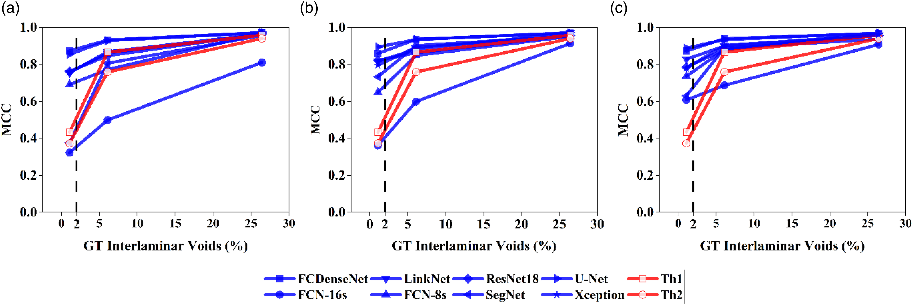

The Deep Learning models were compared to conventional thresholding approaches in Figure 5. Segmentation of the same ROIs was done using the ISO-50% (Th1) and local minimum (Th2) techniques according to the methods outlined in.¹³ Thresholding performance converges towards the Deep Learning segmentation score as the porosity increases, driven by a rise in the precision and recall values. FCN-16s is the only architecture consistently underperforming thresholding in the three regions, regardless of the training set size, except in ROI 1 when using the largest training set. SegNet initially provides a similar MCC score as thresholding but increasing the training set allows the architecture to significantly overperform thresholding methods in ROI 1. U-Net and FCDenseNet are the only Deep Learning models outperforming thresholding in all conditions.

After assessing the location of the mislabelled pixels produced in the segmentation of interlaminar voids in ROI 2 (Figure 6), two observations can be made. On the one hand, the results shown in Table 3 can be visually verified as most of the misabelling occured in the form of false negatives, leading to a decrease of the recall value. On the other hand, the majority of the mislabelled pixels appear around the edges of the voids, i.e., at the interface of two phases. These areas, containing ambiguous grey values, are a challenge in terms of the manual annotation of the ground truth as they lack a high-contrast limit between the two phases. This effect was also mentioned in the Deep Learning phase segmentation of glass-fiber reinforced polyamide 66.²¹

Figure 6.

Visual location of the false positives (red) and false negatives (blue) generated in the segmentation of interlaminar voids in ROI 2 by the eight models and three training set sizes.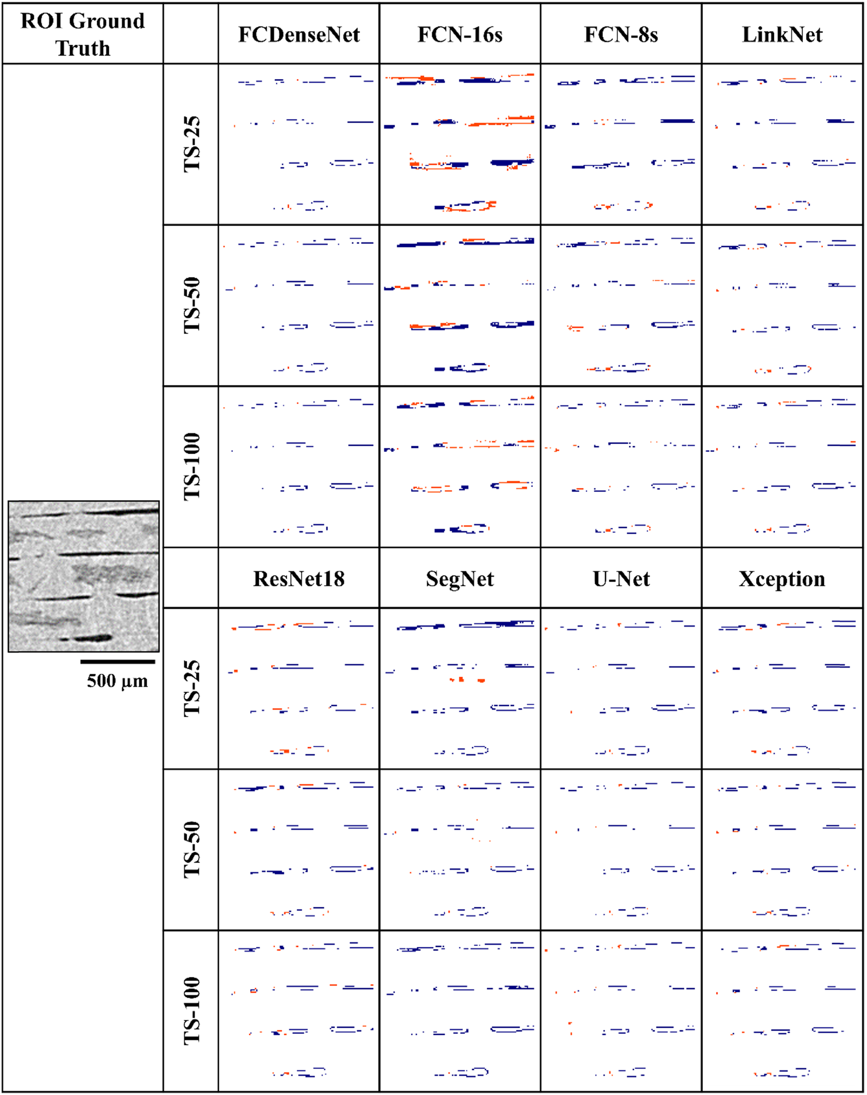

The segmentation performance for the dry areas with increasing training set size is shown in Figure 7. U-Net and FCDenseNet architectures provide the best segmentation, on average, regardless of the training set size. The other six architectures showed a consistent and robust performance in the segmentation of dry areas. All models, except SegNet, showed the strongest results when 100 images were used for training. Overall, the CNNs consistently outperform the thresholding approach, which notably struggles in the correct segmentation of dry areas containing darker pixels.¹³

Figure 7.

Average MCC score achieved by each architecture with respect to the training set size (25, 50 and 100) and thresholding approach for the segmentation of dry areas and calculated across the three ROIs. The error bars represent the standard deviation of the MCC across the three ROIs.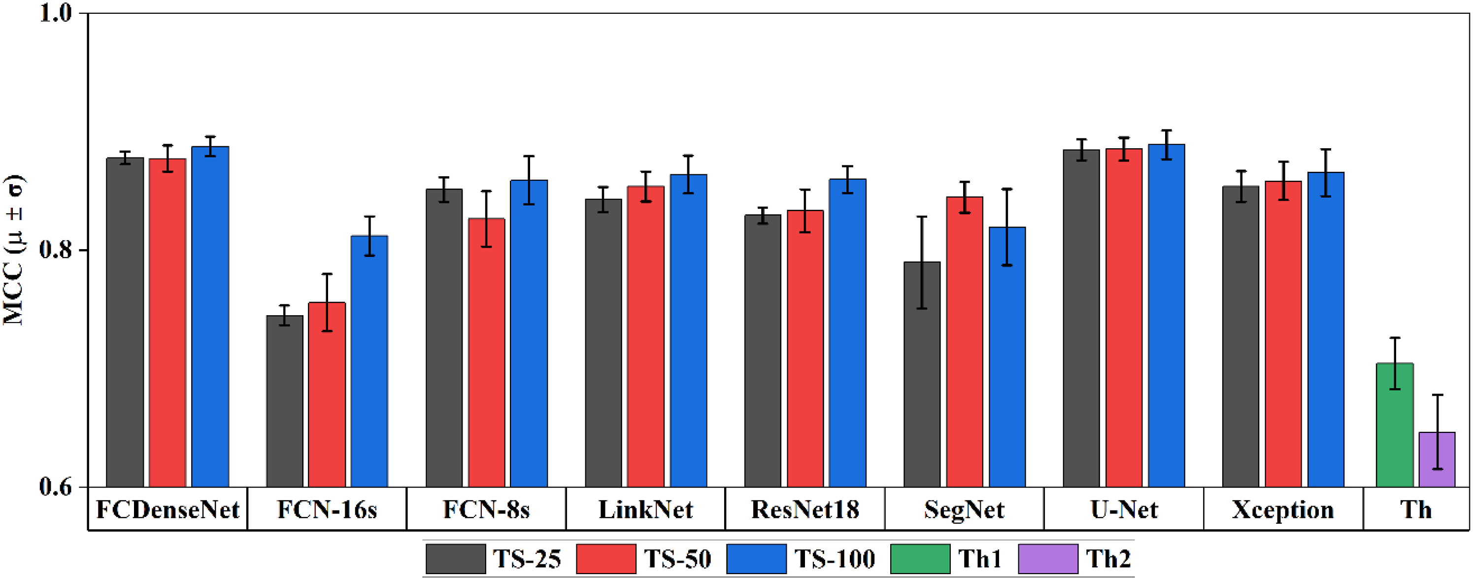

From Figure 8, it was observed that part of the mislabelling is produced by an approximately equal number of false positives and false negatives, which steadily decreases as the training set was increased. It is worth noting that U-Net (TS-25) is the only model to fully segment an unusual thin and diagonal dry area in ROI 2. Most dry areas are orientated horizontally. Further increasing the number of training images caused the U-Net (TS-25) to overlook this feature, in line with the segmentation behaviour showed by the other models. Some models either partially segmented it or produced a full mislabelling in the form of false negatives. A hypothesis derived from this observation is that the ratio of examples of such types of dry areas diminishes as the training set increases, also known as intra-class imbalance,⁶⁰ thus hampering the model learning of such specific typology of dry area.

Figure 8.

Visual location of the false positives (red) and false negatives (blue) generated in the segmentation of dry areas in ROI 2 by the eight models and three training set sizes. The red arow in the greyscale image points to an unusually diagonal and thin dry area.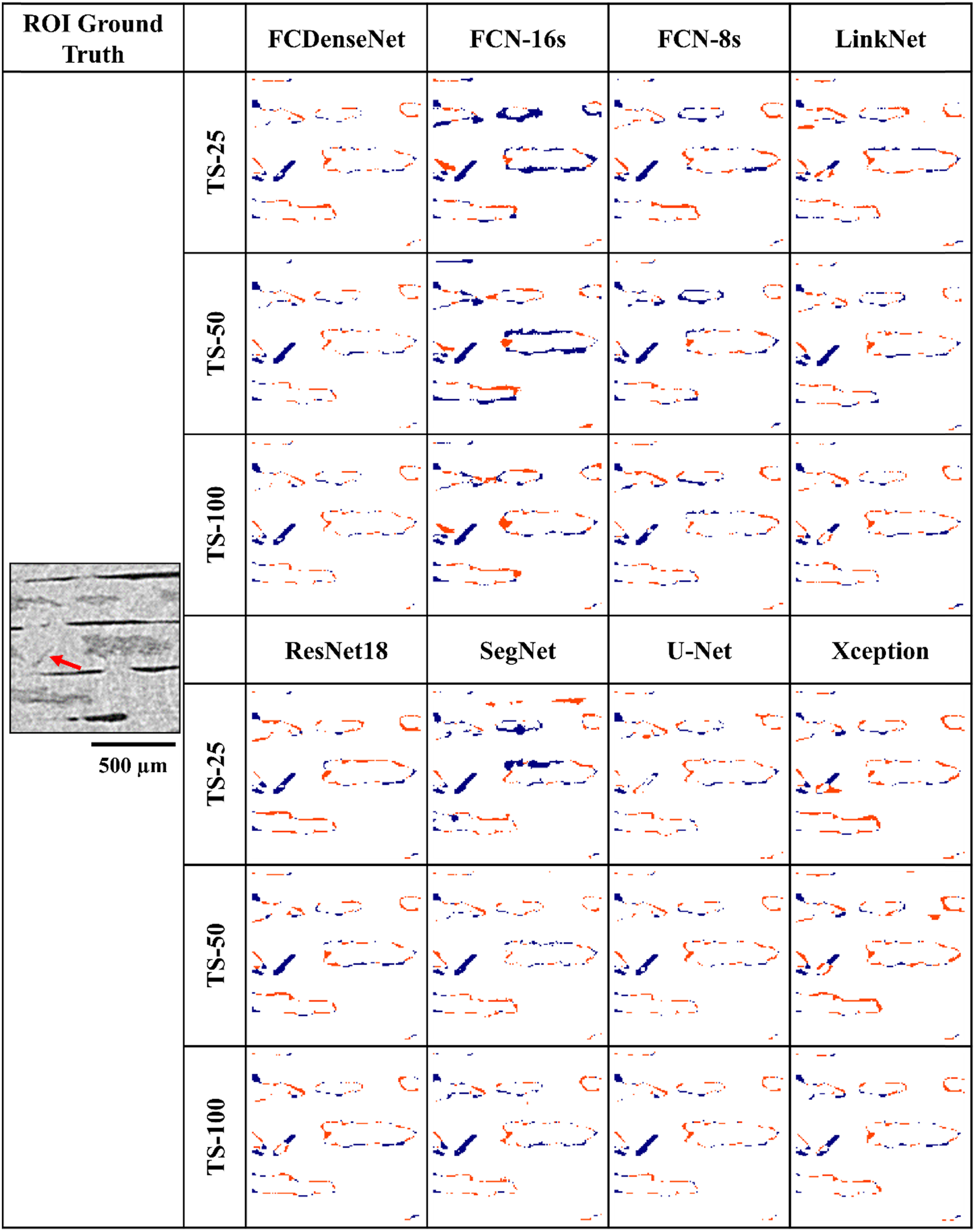

Finally, it was noted that all models were able to identify the noise and artefacts inherent to X-ray imaging and avoid mislabelling voids as dry areas, or vice-versa. This showcases the ability of Deep Learning to handle moderate levels of noise and artefacts and therefore, eliminating the need of applying de-noising filters that involve information loss.

Conclusion

The two main porosity phases (interlaminar voids and dry areas) of an uncured composite laminate were characterised using eight state-of-the-art CNN architectures. Each CNN was trained with three independent training sets containing twenty-five, fifty and one-hundred X-ray micrograph images. The segmentation performance of each model was optimised via a tailored selection of the main set of hyperparameters.

The typology of the CNN architecture and the training set size were found to play a key role in the segmentation accuracy. It was observed that increasing the number of parameters did not necessarily lead to a higher segmentation performance, as was the case for FCN-8s and FCN-16. Additionally, the high performance showed by the U-Net architecture points to the fact that reducing the number of parameters combined with specific strategies aiming to recover feature maps from early stages in the network allows a reduction in the training and prediction time. FCDenseNet provided a comparable segmentation performance as U-Net, with a further reduction of the number of training parameters, but due to the density of the network, the average training and prediction times were significantly increased (+68.5% training time and +21.3% prediction time).

The performance of the models in the segmentation of both porosity phases increased as the ground truth and the training set size increased. In general, the CNN models reached their peak MCC and Dice Coefficient values when a training set size of one hundred images was used. Notably, U-Net and FCDenseNet provided the highest performance in the segmentation of the interlaminar voids, when trained with the smallest image set (25 in this study), achieving only marginal improvements after doubling and quadrupling the number of training images. Similarly, these two architectures also achieve the highest MCC score in the segmentation of dry areas.

Deep learning was found to consistently outperform the established thresholding approach in the segmentation of dry areas because of the wider range of pixel greyscale values. The greyscale value distribution of voids is more pronounced, therefore thresholding fairs somewhat better at segmenting higher porosity (>5%) micrograph images. At low porosity levels (<2%) expected in high-performance composites, most deep learning architectures are superior, with U-Net and FCDenseNet leading the way.

This study has contributed to defining which state-of-the-art CNN architectures achieve the highest performance segmentation of X-ray micrographs, as well as providing guidance on the selection of hyperparameters that produce the best segmentation results. Furthermore, the trade-off between annotation effort, training and prediction time, and segmentation performance was analysed. The U-Net architecture trained with twenty-five images, at the analysed image size and resolution, appears to be a sensible starting point for characterisation of the interlaminar porosity and dry areas of composite materials, while also ensuring a reduction in the training and prediction time. This is needed in quality control processes for high-value composite manufacturing, involving batch-to-batch analysis of incoming prepreg materials or intra-batch variability analysis.

Supplemental Material

Supplemental Material - The effect of convolutional neural network architectures on phase segmentation of composite material X-ray micrographs

Supplemental Material for The effect of convolutional neural network architectures on phase segmentation of composite material X-ray micrographs by Pedro Galvez-Hernandez and James Kratz in Journal of Composite Materials

Footnotes

Acknowledgements

The authors would like to acknowledge the Engineering and Physical Sciences Research Council (EPSRC) for their support of this research through Investigation of Fine-Scale Flows in Composites Processing [EP/S016996/1]. A PhD studentship for P. Galvez-Hernandez was supported through the Rolls-Royce Composites University Technology Centre at the University of Bristol.

Declaration of conflicting interests

The author(s) declared no potential conflicts of interest with respect to the research, authorship, and/or publication of this article.

Funding

The author(s) disclosed receipt of the following financial support for the research, authorship, and/or publication of this article: This study is supported by Engineering and Physical Sciences Research Council (EP/S016996/1).

Data Availability

The raw CT data underlying this article are not available by agreement with our industrial partners to protect their commercial confidentiality.

ORCID iD

James Kratz

Supplemental Material

Supplemental material for this article is available online.

References

Mouritz

. Introduction to aerospace materials. Sawston: Woodhead Publishing Limited, 2012.

LeCun

Bengio

Hinton

. Deep learning. Nature 2015; 521(7553): 436–444.

Goodfellow

Bengio

Courville

. Deep learning. Cambridge: MIT Press, 2017.

Lorenzoni

Curosu

Paciornik

, et al. Semantic segmentation of the micro-structure of strain-hardening cement-based composites (SHCC) by applying deep learning on micro-computed tomography scans. Cement and Concrete Composites 2020; 108: 103551.

Long

. Microscopy cell nuclei segmentation with enhanced U-Net. BMC Bioinformatics 2020; 21(1): 8.

Seah

JCY

Tang

CHM

Buchlak

, et al. Effect of a comprehensive deep-learning model on the accuracy of chest x-ray interpretation by radiologists: a retrospective, multireader multicase study. Lancet Digit Health 2021; 3(8): e496–e506.

Liu

K-W

Yang

, et al. Review of deep learning based automatic segmentation for lung cancer radiotherapy. Front Oncol 2021; 11(2599): 717039.

Gobert

Kudzal

Sietins

, et al. Porosity segmentation in X-ray computed tomography scans of metal additively manufactured specimens with machine learning. Additive Manufacturing 2020; 36: 101460.

Sammons

Winfree

Burke

, et al. Segmenting delaminations in carbon fiber reinforced polymer composite CT using convolutional neural networks. AIP Conference Proceedings 2016; 1706(1): 110014.

10.

Kopp

Joseph

, et al. Deep learning unlocks X-ray microtomography segmentation of multiclass microdamage in heterogeneous materials. Adv Mater 2022; 34: e2107817.

11.

Sinchuk

Kibleur

Aelterman

, et al. Variational and deep learning segmentation of very-low-contrast X-ray computed tomography images of carbon/epoxy woven composites. Materials (Basel) 2020; 13(4): 936.

12.

Ali

Guan

Umer

, et al. Deep learning based semantic segmentation of µCT images for creating digital material twins of fibrous reinforcements. Composites Part A: Applied Science and Manufacturing 2020; 139: 106131.

13.

Galvez-Hernandez

Gaska

Kratz

. Phase segmentation of uncured prepreg X-Ray CT micrographs. Composites Part A: Applied Science and Manufacturing 2021; 149: 106527.

14.

Machado

Tavares

JMRS

Camanho

, et al. Automatic void content assessment of composite laminates using a machine-learning approach. Composite Structures 2022; 288: 115383.

15.

Ronneberger

Fischer

Brox

. U-net: convolutional networks for biomedical image segmentation. In: Navab

Hornegger

Wells

Frangi

(eds). Medical image computing and computer-assisted intervention – MICCAI 2015. Cham: Springer International Publishing, 2015, pp. 234–241.

16.

Jégou

Drozdzal

Vazquez

, et al. The one hundred layers tiramisu: fully convolutional DenseNets for semantic segmentation, 2016.

17.

Badran

Marshall

Legault

, et al. Automated segmentation of computed tomography images of fiber-reinforced composites by deep learning. J Mater Sci 2020; 55(34): 16273–16289.

18.

Luo

Zhang

Lei

, et al. Identification of voids and interlaminar shear strengths of polymer-matrix composites by optical microscopy experiment and deep learning methodology. Polym Adv Technol 2021; 32(4): 1853–1865.

19.

Djavadifar

Graham-Knight

Kӧrber

, et al. Automated visual detection of geometrical defects in composite manufacturing processes using deep convolutional neural networks. J Intell Manuf 2021; 33: 2257–2275.

20.

Fioravante de Siqueira

Ushizima

van der Walt

. A reusable neural network pipeline for unidirectional fiber segmentation. Sci Data 2022; 9(1): 32.

21.

Bertoldo

JPC

Decencière

Ryckelynck

, et al. A modular U-net for automated segmentation of X-ray tomography images in composite materials. Front Mater 2021; 8.

22.

Wolff-Fabris

Lengsfeld

Krämer

. 2 - prepregs and their precursors. In: Lengsfeld

Wolff-Fabris

Krämer

Lacalle

Altstädt

(eds). Composite technology. Hanser, 2016, pp. 11–25.

23.

Bradley

Soutis

, et al. A comparison of different approaches for imaging cracks in composites by X-ray microtomography. Philos Trans A Math Phys Eng Sci 2016; 374(2071): 20160037.

24.

Mehdikhani

Straumit

Gorbatikh

, et al.. Detailed characterization of voids in multidirectional carbon fiber/epoxy composite laminates using X-ray micro-computed tomography. Composites Part A: Applied Science and Manufacturing 2019; 125: 105532.

25.

Dilonardo

Nacucchi

De Pascalis

, et al. High resolution X-ray computed tomography: a versatile non-destructive tool to characterize CFRP-based aircraft composite elements. Composites Science and Technology 2020; 192: 108093.

26.

Kratz

Galvez-Hernandez

Pickard

, et al. Lab-based in-situ micro-CT observation of gaps in prepreg laminates during consolidation and cure. Composites Part A: Applied Science and Manufacturing 2021; 140: 106180.

27.

de Parscau du Plessix

Lefébure

Boyard

, et al. In situ real-time 3D observation of porosity growth during composite part curing by ultra-fast synchrotron X-ray microtomography. Journal of Composite Materials 2019; 53(28–30): 4105–4116.

28.

Garcea

Wang

Withers

. X-ray computed tomography of polymer composites. Composites Science and Technology 2018; 156: 305–319.

29.

Schindelin

Arganda-Carreras

Frise

, et al. Fiji: an open-source platform for biological-image analysis. Nat Methods 2012; 9(7): 676–682.

30.

Long

Shelhamer

Darrell

. Fully convolutional networks for semantic segmentation. Piscataway, NJ: IEEE, 2014.

31.

Kaymak

Ucar

. Skin lesion segmentation using fully convolutional networks: a comparative experimental study. Expert Systems with Applications 2020; 161: 113742.

32.

Piramanayagam

Saber

Schwartzkopf

, et al. Supervised classification of multisensor remotely sensed images using a deep learning framework. Remote Sensing 2018; 10(9): 1429.

33.

Badrinarayanan

Kendall

Cipolla

. SegNet: a deep convolutional encoder-decoder architecture for image segmentation. IEEE Trans Pattern Anal Mach Intell 2017; 39(12): 2481–2495.

34.

Almotairi

Kareem

Aouf

, et al. Liver tumor segmentation in CT scans using modified SegNet. Sensors 2020; 20(5): 1516.

35.

Gómez-Flores

Coelho de Albuquerque Pereira

. A comparative study of pre-trained convolutional neural networks for semantic segmentation of breast tumors in ultrasound. Comput Biol Med 2020; 126: 104036.

36.

Lobo Torres

Queiroz Feitosa

Nigri Happ

, et al. Applying fully convolutional architectures for semantic segmentation of a single tree species in urban environment on high resolution UAV optical imagery. Sensors 2020; 20(2): 563.

37.

Weng

Xia

, et al. Water areas segmentation from remote sensing images using a separable residual SegNet network. ISPRS Int J Geoinf 2020; 9(4): 256.

38.

Wang

Zeng

Liao

, et al. B-FGC-Net: a building extraction network from high resolution remote sensing imagery. Remote Sensing 2022; 14(2): 269.

39.

Ruiz-Santaquiteria

Bueno

Deniz

, et al. Semantic versus instance segmentation in microscopic algae detection. Engineering Applications of Artificial Intelligence 2020; 87: 103271.

40.

Bellens

Probst

Janssens

, et al. Evaluating conventional and deep learning segmentation for fast X-ray CT porosity measurements of polymer laser sintered AM parts. Polymer Testing 2022; 110: 107540.

41.

Eliasson

Karlsson Hagnell

Wennhage

, et al. A statistical porosity characterization approach of carbon-fiber-reinforced polymer material using optical microscopy and neural network. Materials 2022; 15(19): 6540.

42.

Huang

Liu

van der Maaten

, et al. Densely connected convolutional networks. Piscataway, NJ: IEEE, 2016.

43.

Chaurasia

Culurciello

. LinkNet: exploiting encoder representations for efficient semantic segmentation. Piscataway, NJ: IEEE, 2017.

44.

Ribeiro

Avila

Valle

. Less is more: sample selection and label conditioning improve skin lesion segmentation. In IEEE/CVF conference on computer vision and pattern recognition workshops (CVPRW)2020, Seattle, WA, USA, June 2020, pp. 3182–3191.

45.

Tschandl

Sinz

Kittler

. Domain-specific classification-pretrained fully convolutional network encoders for skin lesion segmentation. Comput Biol Med 2019; 104: 111–116.

46.

Shvets

Rakhlin

Kalinin

, et al. Automatic instrument segmentation in robot-assisted surgery using deep learning. Piscataway, NJ: IEEE, 2018.

47.

Chen

L-C

Zhu

Papandreou

, et al. Encoder-decoder with atrous separable convolution for semantic image segmentation. In: Ferrari

Hebert

Sminchisescu

Weiss

(eds). Computer vision – ECCV 2018. Cham: Springer International Publishing, 2018, pp. 833–851.

48.

Zhang

Ren

, et al. Deep residual learning for image recognition. Piscataway, NJ: IEEE, 2015.

49.

Chen

L-C

Papandreou

Schroff

, et al. Rethinking atrous convolution for semantic image segmentation. Piscataway, NJ: IEEE, 2017.

50.

Ali

Guan

Umer

, et al. Efficient processing of μCT images using deep learning tools for generating digital material twins of woven fabrics. Composites Science and Technology 2022; 217: 109091.

51.

Chollet

. Xception: deep learning with depthwise separable convolutions. Piscataway, NJ: IEEE, 2016.

52.

Abadi

Agarwal

Barham

, et al. TensorFlow: large-scale machine learning on heterogeneous distributed systems. NewYork: ACM, 2016.

53.

Bormann

, https://github.com/fabianbormann/Tensorflow-DeconvNet-Segmentation/blob/master/DeconvNet.py (2016).

54.

Fan

, https://github.com/luofan18/linknet-tensorflow/blob/master/code/linknet.py. 2019.

55.

Zakirov

, https://github.com/bonlime/keras-deeplab-v3-plus/blob/master/model.py (2019).

56.

Mathworks , https://uk.mathworks.com/help/vision/ref/deeplabv3pluslayers.html (2022).

57.

TensorFlow SIG addons . 0.14.0 ed.

58.

Noh

Hong

Han

. Learning deconvolution network for semantic segmentation. Piscataway, NJ: IEEE, 2015.

59.

Stan

Thompson

Voorhees

. Optimizing convolutional neural networks to perform semantic segmentation on large materials imaging datasets: X-ray tomography and serial sectioning. Materials Characterization 2020; 160: 110119.

60.

Liu

Wei

, et al. Handling inter-class and intra-class imbalance in class-imbalanced learning. arXiv, 2021.

61.

Breheret

. Pixel annotation tool. GitHub, 2017.

62.

Dutta

Zisserman

. The VIA annotation software for images, audio and video. NewYork: ACM, 2019.

63.

Kornilov

Safonov

Yakimchuk

. A review of watershed implementations for segmentation of volumetric images. J Imaging 2022; 8(5): 127.

64.

OpenCV . Miscellaneous image transformations. 3.1.0 ed.

65.

James

Pruyne

Stan

, et al.. Segmentation of tomography datasets using 3D convolutional neural networks. Computational Materials Science 2023; 216: 111847.

66.

Bengio

. Practical recommendations for gradient-based training of deep architectures. arXiv, 2012.

67.

Kingma

. Adam: a method for stochastic optimization. arXiv, 2014.

68.

Robbins

Monro

. A stochastic approximation method. Ann Math Statist 1951; 22: 400–407.

69.

Duchi

Hazan

Singer

. Adaptive subgradient methods for online learning and stochastic optimization. Journal of Machine Learning Research 2011; 12: 2121–2159.

70.

Tieleman

Hilton

. Lecture 6.5 - RMSProp. COURSERA: neural networks for machine Learning. California: Coursera, 2012.

71.

Ioffe

Szegedy

. Batch normalization: accelerating deep network training by reducing internal covariate shift. arXiv, 2015.

72.

Roberts

Haile

Sainju

, et al. Deep learning for semantic segmentation of defects in advanced STEM images of steels. Sci Rep 2019; 9(1): 12744.

73.

Doube

. Multithreaded two-pass connected components labelling and particle analysis in ImageJ, 2020.

74.

Sørensen

. A method of establishing groups of equal amplitude in plant sociology based on similarity of species content and its application to analyses of the vegetation on Danish commons. København: I kommission hos E. Munksgaard, 1948.

75.

Dice

. Measures of the amount of ecologic association between species. Ecology 1945; 26(3): 297–302.

76.

Matthews

. Comparison of the predicted and observed secondary structure of T4 phage lysozyme. Biochim Biophys Acta 1975; 405(2): 442–451.

77.

Lian

Liu

. Revisit batch normalization: new understanding from an optimization view and a refinement via composition optimization. arXiv, 2018.

Supplementary Material

Please find the following supplemental material available below.

For Open Access articles published under a Creative Commons License, all supplemental material carries the same license as the article it is associated with.

For non-Open Access articles published, all supplemental material carries a non-exclusive license, and permission requests for re-use of supplemental material or any part of supplemental material shall be sent directly to the copyright owner as specified in the copyright notice associated with the article.

0.00 MB

0.27 MB