Sage Journals: Discover world-class research

Abstract

Curing of composite laminates in a vessel was investigated in this study. The environment inside the processing vessel dictates the efficiency and ultimately drives the quality of thermoset composite parts. Experimental measurements of spatial heat transfer coefficients were conducted on industrial scale vessels, including autoclaves and large ovens, which ultimately drives the quality of thermoset composite parts. The final part quality was investigated using the experimental data as input to a coupled heat transfer and curing model. Measurements showed that heat transfer coefficients in autoclaves were greater in magnitude and spatial variability. The distribution in the autoclaves followed a pattern common in the literature, in contrast to that in the ovens which varied considerably between devices. Numerical predictions indicated autoclave measured heat transfer coefficients provide less lag to the imposed temperature history and smaller temperature overshoots. However, the greater robustness to variability at autoclave heat transfer coefficients was offset by the greater variability, resulting in comparable robustness across the ovens and autoclaves.

Keywords

Heat transfer coefficient curing variability autoclave oven thermoset laminate

Introduction

The central element in processing thermoset laminates is the application of heat, this triggers the curing reaction through which desirable properties are acquired. Historically, aerospace grade thermoset laminates have been processed in autoclaves, where the ability to apply a compaction pressure in addition to temperature provides superior consolidation in the final part.¹ More recently, the desire to produce larger parts with less energy and cost has motivated the use of Out-Of-Autoclave manufacturing.² This work focuses on vacuum bag only oven consolidation, where the available compaction pressure is limited to 1 atm. As will be discussed, the inability to apply higher pressure can have negative consequences beyond just poor consolidation.

Material manufacturers often provide a recommended set of processing conditions for a material, this will include a temperature and a pressure cycle (the latter if an autoclave is recommended). However, having the processing environment in-line with these recommendations is not sufficient for producing quality parts. In autoclaves and ovens, forced convection is typically the main source of heat transfer into a part, therefore, it also largely controls the rate of chemical and physical transformation during cure.³ Measurements by Kluge et al.⁴ showed significant temperature differences across a tool in an autoclave, demonstrating the consequences of HTC variation. Through analysing large quantities of defect data Wang et al.⁵ found the failure to achieve a homogeneous cure within a part can induce voids, resin rich regions, pores and delamination, and excessive temperature overshoots have also been observed.⁶

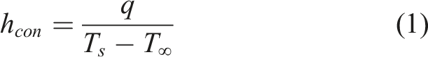
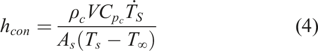
The effectiveness of convective heat transfer from the vessel gas to the part is classically modelled using the convective heat transfer coefficient h_con (HTC). HTC is defined as

h_{c o n} = \frac{q}{T_{s} - T_{\infty}}

(1)

where q is the heat flux across the boundary in Wm⁻²K⁻¹, T_s is the surface temperature and T_∞ is the surrounding gas temperature.

Given the importance of convective heat transfer, studies have been conducted to understand how the value of HTC can vary within an autoclave, Ghamlouch³ presented a comprehensive overview. This analysis routinely involves lumped mass calorimeters. The use of plate calorimeters is common, these are typically insulated at the edges to allow the assumption of 1-dimensional (1D) heat transfer, the validity of these assumptions was demonstrated by Bohne et al.⁷ using Finite Elements (FE). Measurements are taken using thermocouples at locations along the length of the plate. Slesinger et al.⁶ demonstrated that calorimeters consisting of a cylindrical metal rod could produce similar results to a plate, which is advantageous due to the much smaller size. It was through measurements made in this fashion that the connection was demonstrated between the local velocity field and the value of HTC,^3,8 the typical lack of uniformity in autoclave gas flow fields⁶ explaining the large amounts of observed variability.

A number of studies have focused on providing detailed analysis of the thermal environment within autoclaves.^4,6,9–11 Studies mapping the distribution of HTC within an autoclave consistently found large spatial variations. For example, Slesinger et al.⁶ found a variation from 60 to 200 Wm⁻²K⁻¹ in a 1.5 m long autoclave with a 1.15 m diameter and Bohne et al.⁷ found a variation from 70 to 110 Wm⁻²K⁻¹ in a 2 m long autoclave with a 1 m diameter. In the study by Kluge et al.,⁴ it was noted spatial HTC values appear to depend on the configuration of the autoclave, increasing pressure or flow velocity augments them while maintaining the existing pattern.

Autoclave layouts generally vary little from that shown in Figure 1, as such there has been an agreement between the HTC distributions reported by different studies, higher values are found at the front and decrease towards the back as the high velocity inlet air recirculates off the door and flows to the recirculating fan at the back of the vessel.^3,12 This deduced flow pattern has been confirmed using CFD analysis.⁶ Johnston¹³ demonstrated the need to consider multiple devices to deduce general relationships, when one of the three autoclaves considered showed a contradictory decrease in HTC at higher pressures, this was attributed to insufficient fan power to accommodate the resulting air density increase.

Figure 1.

Images of two of the studied vessels, oven 5 (left) and autoclave 1 (right).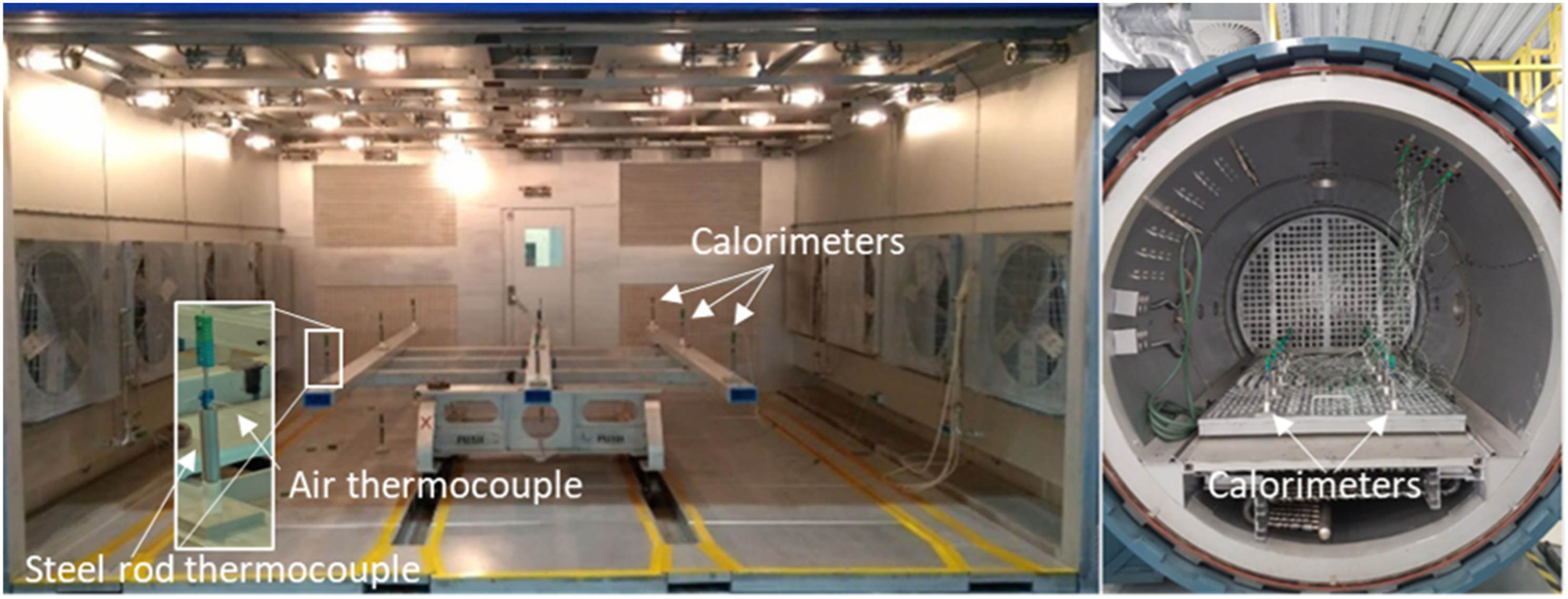

Despite the increasing use of ovens for processing composites, there appears to be no analysis of the HTC distribution within ovens analogous to the autoclave examples given above. This is surprising given the lack of applied pressure causes variability in the processing environment to have more influence on the properties of the final part. This was demonstrated by Kluge et al.,⁴ when applying the same temperature history with and without applied pressure it was found that the application of pressure significantly reduced the front-back temperature difference in the tool. The greater sensitivity of HTC to pressure compared to the temperature history in autoclaves has been widely reported.^7,13

Motivated by this absence in the literature, the first part of this study includes the analysis of HTC in ovens. The work presented shows the dependence of HTC on internal geometry and the gas circulatory system.³ To verify this for ovens, a range of oven sizes is considered, and particular attention is given to the influence of features such as shape, size, inlet, and exhaust locations. For comparison, the HTC distributions inside two autoclaves are also considered. Mapping the devices under the same conditions enables any common trends and differences to be identified, allowing a distinction to be made between what can be assumed to be generally applicable and what must be considered on a case-by-case basis.

The resulting properties of a part manufactured in such a vessel are linked to the mechanics during the curing process.¹⁴ At gelation, the degree of cure (DOC) the resin transitions between a viscous and a rubbery state, there are significant changes in material properties, including shrinkage and the ability to sustain stresses.¹⁵ For a given resin system chemistry, the time for gelation to occur depends on temperature history,¹⁶ hence temperature gradients can lead to non-uniformities through the material.^17,18 Thus, to fully understand the effect of heat transfer variability on the final part, cure kinetics must be considered. Given the cure kinetics are driven by heat transfer in the material, a coupled approach, first proposed by Loos and Springer,¹⁹ is required to predict the phenomena.

To understand the consequence of HTC nonuniformity on the curing reaction, in the second part of this study, an FE model will be used to solve coupled heat transfer and cure kinetics equations. Laminate thickness is typically much smaller than the in-plane dimensions, enabling an efficient 1D modelling through thickness. Five indicators shall be considered to capture the influence of HTC variability on the curing process, two refer to the transverse temperature distribution in isolation, the other three take cure kinetics into account.

In consideration of heat transfer, the lag between the imposed conditions and those in the laminate, and the uniformity of conditions within the laminate shall be studied. In consideration of cure kinetics, processing efficiency, the likelihood of residual stresses, and excessive temperature will be the focus. Measured HTC data from the different vessels is used in the FE model to investigate the distinctions between curing in an oven and an autoclave.

Experimental mapping of HTC in ovens and autoclaves

Methods

Temperature measurements

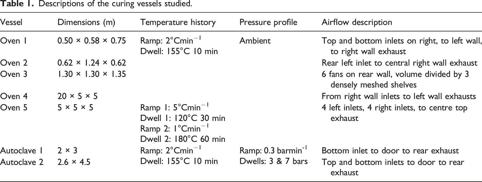
Calorimeter measurements were taken in seven vessels: five ovens and two autoclaves. Descriptions of each vessel and the measurement conditions are provided in Table 1. Figure 1 shows examples of how measurements were taken in the ovens and autoclaves, the images demonstrate the arrays of calorimeters used to take temperature measurements at fixed sets of locations within the volumes of each vessel, apart from which they were empty. Note that although this indicated the expected level of variability within the vessels, in practice the moulds and parts will have a strong influence on the flow conditions,¹³ which is not captured here.

Table 1.

Descriptions of the curing vessels studied.

Vessel	Dimensions (m)	Temperature history	Pressure profile	Airflow description
Oven 1	0.50 × 0.58 × 0.75	Ramp: 2°Cmin⁻¹ Dwell: 155°C 10 min	Ambient	Top and bottom inlets on right, to left wall, to right wall exhaust
Oven 2	0.62 × 1.24 × 0.62			Rear left inlet to central right wall exhaust
Oven 3	1.30 × 1.30 × 1.35			6 fans on rear wall, volume divided by 3 densely meshed shelves
Oven 4	20 × 5 × 5			From right wall inlets to left wall exhausts
Oven 5	5 × 5 × 5	Ramp 1: 5°Cmin⁻¹ Dwell 1: 120°C 30 min Ramp 2: 1°Cmin⁻¹ Dwell 2: 180°C 60 min		4 left inlets, 4 right inlets, to centre top exhaust
Autoclave 1	2 × 3	Ramp: 2°Cmin⁻¹ Dwell: 155°C 10 min	Ramp: 0.3 barmin^-1 Dwells: 3 & 7 bars	Bottom inlet to door to rear exhaust
Autoclave 2	2.6 × 4.5	Ramp: 2°Cmin⁻¹ Dwell: 155°C 10 min	Ramp: 0.3 barmin^-1 Dwells: 3 & 7 bars	Top and bottom inlets to door to rear exhaust

Heat transfer coefficient estimation

The calorimeters, assumed to be lumped masses, consisted of two K-type thermocouples, one inside a stainless-steel 304 rod of length 0.1 m and diameter 0.025 m, the other on the outside to measure the local air temperature. The temperature measurements from the two thermocouples enabled a global calorimeter HTC to be estimated through the following procedure.

Total heat 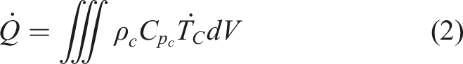$\dot{Q}$ input in the calorimeter can be determined for a given temperature increase $\dot{T_{C}}$ as

\dot{Q} = ∭ ρ_{c} C_{p_{c}} \dot{T_{C}} d V

(2)

where ρ_c is the density,

C_{p_{c}}

is the specific heat capacity and T_c is the temperature of the calorimeter. Temperature was considered uniform in the calorimeters, the integral became equivalent to

\dot{Q} = ρ_{c} V C_{p_{c}} \dot{T_{S}}

(3)

where V is the calorimeter volume and for convention, T_s is the calorimeter surface temperature. Substituting this simplified form into equation (1) yielded the expression that was used to compute the HTC from the experimental data

h_{c o n} = \frac{ρ_{c} V C_{p_{c}} \dot{T_{S}}}{A_{s} (T_{s} - T_{\infty})}

(4)

where A_s is the calorimeter surface area. The temperature data (T_s,T_∞) used to calculate the HTC was limited to that of the thermocouples during the ramp up. During this sliding regime,

T_{s} - T_{\infty}

was approximately constant for all calorimeters, with the standard deviations typically around 2°C. The reported value of HTC for each set of calorimeter measurements was the mean of all the values computed during this period. Assuming noise to be random, this approach helped to reduce the influence of the noise from the thermocouple measurements. In the case of oven 5, the measurements from the first ramp (Table 1) were used due to the superior quality of the recorded data.

Validating the lumped mass assumption

Biot number is defined as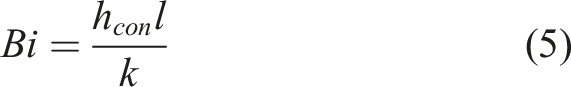

B i = \frac{h_{c o n} l}{k}

(5)

where h_con is HTC, l and k are the characteristic length and thermal conductivity of the object. The characteristic length can be taken as the ratio of volume to surface area, for a cylinder this is equal to half the radius. The horizontal surfaces of the cylinders were partially obscured, to be conservative, they were not accounted for. The cylinders had radii of 0.0125 m and thermal conductivities of 14 Wm⁻¹K⁻¹, this gave a Biot number of roughly 0.00045 h_con. For Biot numbers below 0.1 a uniform temperature assumption is valid.²⁰ This gave a maximum allowable HTC of 224 Wm⁻²K⁻¹. Given the greatest measured HTCs of 203 Wm⁻²K⁻¹ and 62 Wm⁻²K⁻¹ in the autoclaves and ovens respectively, the assumption was valid in both vessels.

Checking for negligible radiative heat transfer

Radiative heat transfer is computed according to the Stefan-Boltzmann law of radiation

q_{r a d} = ε σ ({T_{w a l l}}^{4} - {T_{c a l}}^{4})

(6)

where q_rad is the heat flux into the calorimeter,

ε

is the calorimeter emissivity, T_cal and T_wall are the temperatures of the calorimeter and wall respectively, and

σ

is the Stefan-Boltzmann constant. When the mean (T_m) of T_cal and T_wall is much greater than the difference between them (∆T) (i.e.

{(∆ T / T_{m})}^{2} / 4 ≪ 1

), which is the case here, equation (6) can be linearised into the same form as equation (1).²¹ As the calorimeters are much smaller than the vessels, the view factor can be omitted and the resulting coefficient of radiative heat transfer writes

h_{r a d} = 4 σ T_{m}^{3} ε

(7)

The calorimeters were stainless steel 304 which has emissivity between 0.32 and 0.38.^22,23 To be conservative, the upper bound, $ε = 0.38$ , was assumed.

To be conservative, T_wall was assumed equal to the air temperature. The ratio of h_con to h_rad was between 3 and 15 in the ovens and between 160 and 650 in the autoclaves. In line with the literature for similar ratios,²⁴ it was deemed acceptable to assume h_con was the sole contribution to HTC (h) in both sets of vessels.

Experimental results

HTC variability between the vessels

The temperature and pressure dependence of HTC in turbulent flow is¹³

h \propto {(\frac{p}{T})}^{\frac{4}{5}}

(8)

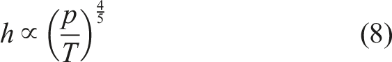
This indicates the results from oven 5 are not directly comparable to the others due to the different temperature history used, they are included as a further example. Conversely, literature^7,13 suggests when the relative change in pressure is much greater than temperature, as in the autoclave cycles, HTC can be approximated solely as a linear function of pressure, the dependence on temperature and heating rate being minor.

The measured HTC values in addition to data from Slesinger⁶ are summarised in Figure 2, the plotted values are the means, and the error bars represent the standard deviations taken over the calorimeters in each vessel. The error bars at 1 and 7 bars represent the standard deviation of HTC for all the vessels at these pressures to aid visualisation. The pressure dependence of HTC described in equation (8) is shown to follow the general trend of the measurements. A fitting coefficient of 29.3 was found to minimise the mean squared error between equation (8) and the measurements.

Figure 2.

Spatial means of HTC measurements in each vessel during the two trials along with autoclave data from Slesinger.⁶ Equation (8) model fit is also plotted. The error bars signify the standard deviations of the measurements. At 1 and 7 bars respectively, the error bar is the standard deviation of all the oven and autoclave data centred at the mean HTC.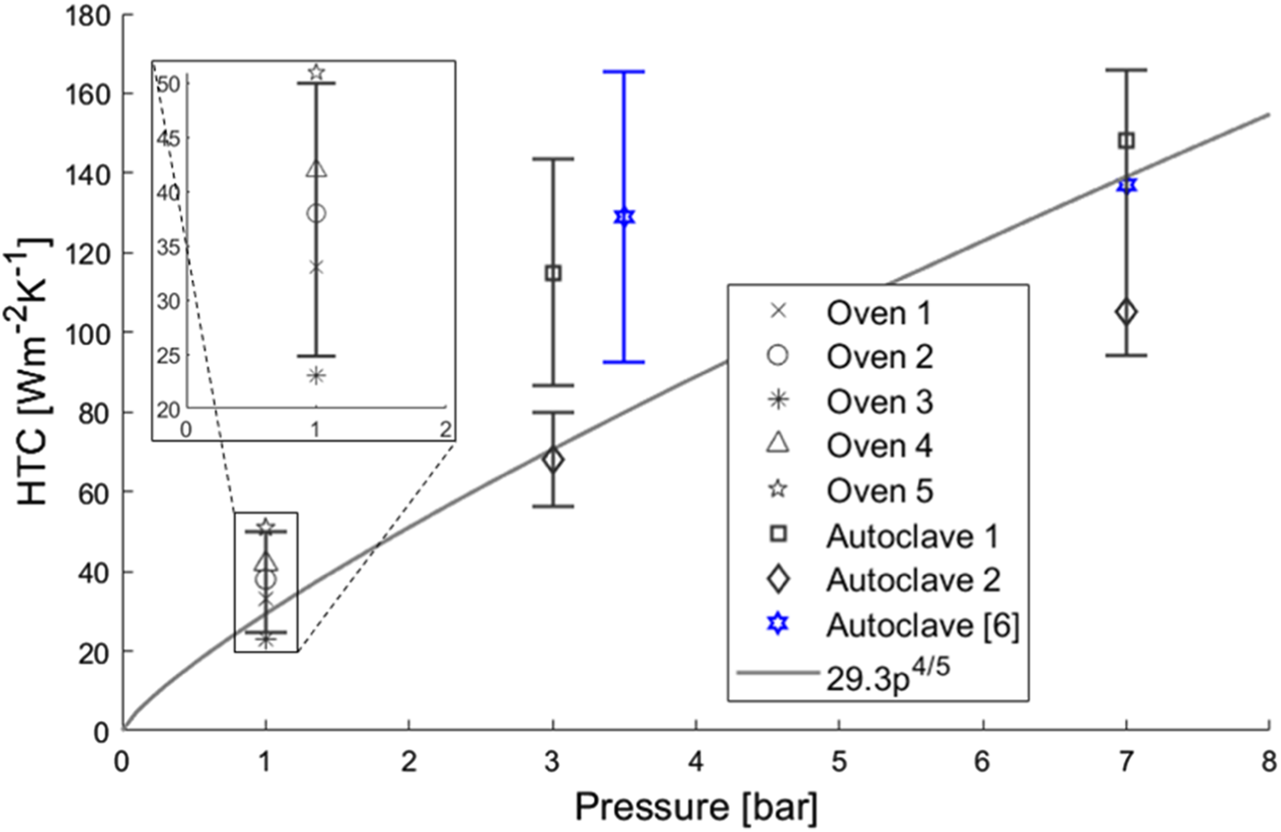

The results showed little difference between the mean HTC in each trial for all vessels. This result reflects the conclusions from autoclave measurements in the literature which showed little change under constant pressure.⁷ Run-to-run variability is lowest in the ovens followed by the autoclaves at 3 and 3.5 bars. In all autoclaves the run-to-run difference increased at 7 bars. This trend can be interpreted using the link between the gas flow and HTC. Air density increases with pressure, Reynolds number is proportional to density, therefore, the less repeatable HTC distributions at elevated pressure result from greater turbulence in the gas flow.

The effect of applied pressure is clear when the mean HTC values from the ovens are compared with those from the autoclaves. The autoclaves have greater values in all cases, particularly when operated at 7 bars. This trend is to be expected given equation (8), however the results suggest this relationship has a tendency to overpredict the influence of pressure. When scaled accordingly, the HTC predicted for the oven data consistently exceeded the values measured in the autoclaves, indicating the presence of other influential factors, for example the more significant radiative contribution to the oven measured HTC. The greater HTC in the large ovens is likely due to more powerful gas circulatory systems providing higher air speeds.

Spatial HTC variability within the vessels

The standard deviations displayed in Figure 2 represent the spatial variability in HTC during the two trials. Interestingly, in the oven data, there is no clear relationship between size and the level of spatial variability, the second smallest oven produced the lowest standard deviation, yet the largest oven displayed a lower value than the smallest oven. The absence of a standard configuration among ovens likely contributed to the lack of consistency. The large value for Oven 5 was due to a single extreme measurement, which was attributed to the proximity of the calorimeter to the exhaust, discounting this gives the more reasonable standard deviation of 4.1 Wm⁻²K⁻¹. Among the three autoclaves in Figure 2, there is a trend towards decreasing spatial variability with increasing size.

There is a noticeable difference between the observed spatial variability in the ovens compared to the autoclaves. This difference can likely be attributed to the techniques used to achieve high HTC in the autoclaves. In addition to elevated pressure, HTC and Reynolds number are positively correlated with air velocity, motivating high inlet air speeds. Due to the way air flows are generally setup in autoclaves³ this causes a big contrast in the airspeed at the front to that at the back, producing the high spatial variability in HTC.

To provide a summary of the spatial HTC variability within the ovens and autoclaves more generally, Figure 3 presents a boxplot of the measurement grouped by vessel type. The autoclave measurements at the different pressures are treated separately due to the strong influence of pressure on HTC. The large range of values measured in the autoclaves is consistent with the literature.^6,7 The largest HTC values occurred around the front and the smallest at the back in accordance with the air flow pattern discussed above. When comparing the oven results with the autoclave results, and the 3 bars autoclave with the 7 bars autoclave results, an apparent trend emerges with greater pressure resulting in a broader range of measured values. Despite this, in the autoclaves, the spatial variability represented by the inter-quartile range appears to be unaffected by the change in pressure, this latter result supports the literature^4,13 which reported the preservation of patterns in the HTC field with changes in pressure.

Figure 3.

Measured HTC values in the ovens and the autoclaves.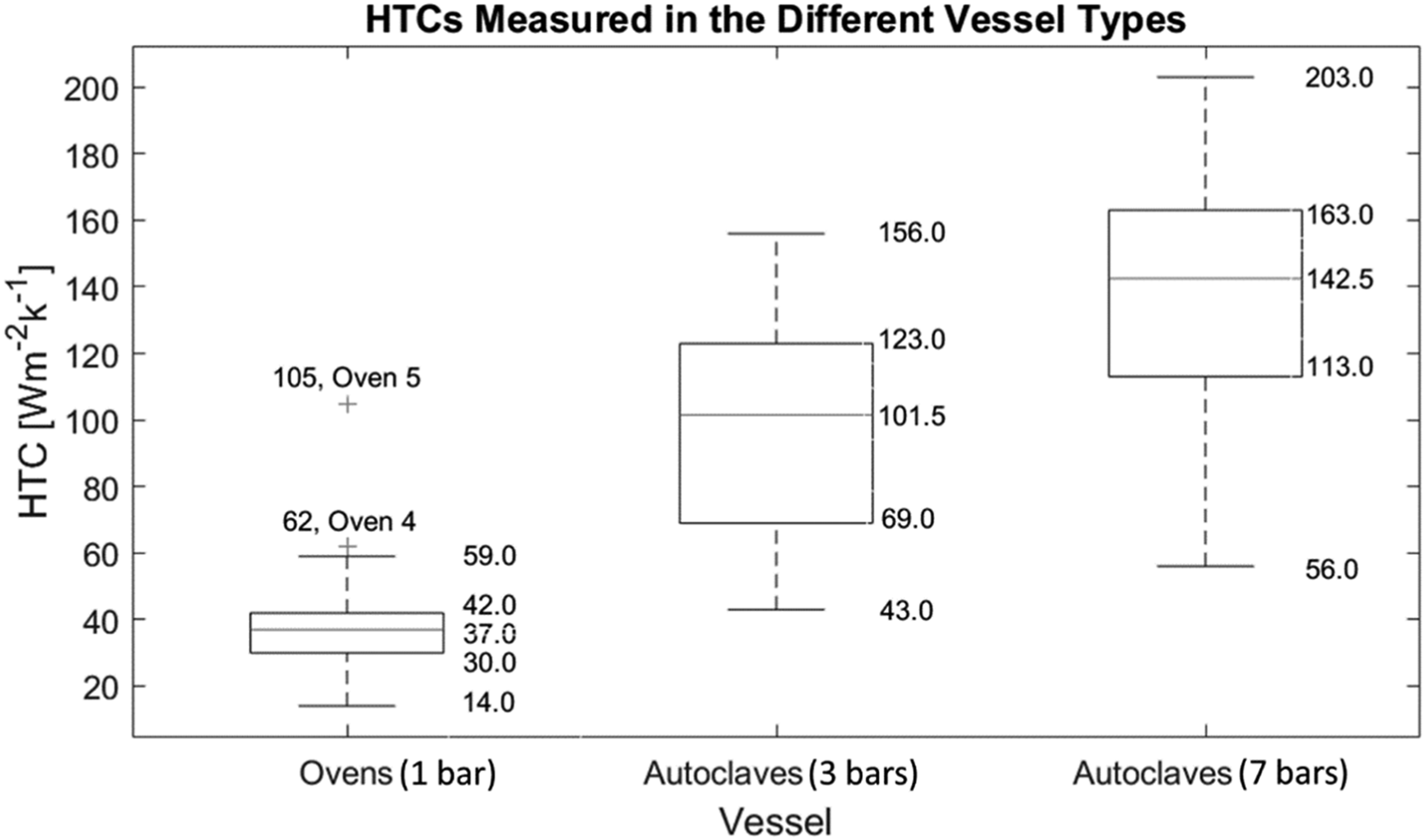

The spatial disparities observed in the ovens were generally smaller. The uniquely large maximum HTC of 105 Wm⁻²K⁻¹ in oven 5 (the second largest was 51 Wm⁻²K⁻¹) was the cause of the large variability presented in Figure 2. The smaller inter-quartile range of the oven data reflects the low spatial variability measured in the ovens. The skew of the oven data towards higher values is due to the lower values (<24 Wm⁻²K⁻¹) being solely contributed by oven 3, the size of these measurements was attributed to the shelves which would have obstructed the airflow, lowering the velocity. Lacking a standard configuration like the autoclaves, the recorded HTC field patterns varied among the ovens, in practice this necessitates a case-by-case approach to analysis of oven environments.

Numerical methods and results

Numerical modelling

Coupled cure kinetics and transient heat transfer equations were solved using the FE method to capture the curing process through the thickness of a carbon fibre reinforced thermoset laminate.

Numerical implementation

The curing process of the thermoset laminate was modelled using FE in COMSOL Multiphysics to solve coupled heat transfer and cure kinetics equations. The cure kinetics model was derived by Mesogitis et al.²⁵ by fitting differential scanning colorimeter data to an adapted version of the Kamal and Sourour model²⁶ and was validated against experimental data.

It was assumed that the in-plane dimensions of the laminate far exceeded the thickness, hence the in-plane temperature gradients could be treated as negligible, allowing a 1D approximation of heat transfer.²⁷ Furthermore, spatial variability in HTC will have a negligible effect on the in-plane temperature gradient compared to the transverse gradient.

The geometry of the 1D model is represented in Figure 4, it consisted of a homogenised thermoset composite laminate in ideal contact with a 10 mm thick invar tool. The origin was taken to be at the interface between the two domains, this approach facilitated independent analysis of the two domains.

Figure 4.

The geometry used in the FE model.

The properties of the homogenised laminate were representative of Hexply M21 carbon fibre epoxy prepreg.^25,28 Simulations were performed with part thicknesses of 5 mm, 10 mm and 15 mm. These specific geometries were considered for illustrative purposes. It is noted that although the trends will be applicable, any such example will lack generality due to the strong influence of geometric parameters such as the laminate and tool thicknesses on the curing process.⁶

The heat transfer component of the model was implemented using the ‘Heat Transfer in Solids’ physics in COMSOL. The heat equation is a first order in time and second order in space partial differential equation, therefore requires an initial condition and two boundary conditions to solve. The initial condition was that the system started at a temperature of 20°C. The boundary conditions were convective, applied to the two ends of the geometry. The air temperature history followed by $T_{\infty}$ during this study was based on the recommended cycle for Hexply M21.²⁸ It consisted of a 2°C per minute ramp from 20°C followed by a dwell at 180°C for 2 hours, which is a typical curing cycle for aerospace grade epoxy systems.

The cure kinetics model was implemented in COMSOL as a distributed ordinary differential equation applied to the laminate domain. Computations were performed assuming an initial degree of cure of 0.01 to escape the singular stationary point of the model.

The implementation of the coupled model into COMSOL was validated through a comparison with experimental data.²⁵

Dimensional analysis

As detailed in the appendix, the dimensionless forms of the heat equations applied to the laminate and tool domains respectively were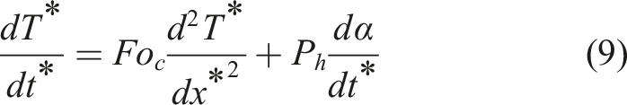

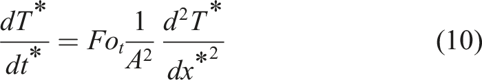
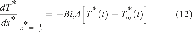
\frac{d T^{*}}{d t^{*}} = F o_{c} \frac{d^{2} T^{*}}{d {x^{*}}^{2}} + P_{h} \frac{d α}{d t^{*}}

(9)

\frac{d T^{*}}{d t^{*}} = F o_{t} \frac{1}{A^{2}} \frac{d^{2} T^{*}}{d {x^{*}}^{2}}

(10)

where

F o_{c}

and

F o_{t}

are the composite and tool Fourier numbers respectively, A is the laminate to tool thickness ratio and

P_{h}

is the phase transition number.

The convective boundary conditions applied to the free edge of the laminate and tool domains became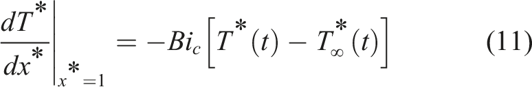

{\frac{d T^{*}}{d x^{*}} |}_{x^{*} = 1} = - B i_{c} [T^{*} (t) - T_{\infty}^{*} (t)]

(11)

{\frac{d T^{*}}{d x^{*}} |}_{x^{*} = - \frac{1}{A}} = - B i_{t} A [T^{*} (t) - T_{\infty}^{*} (t)]

(12)

where

B i_{c}

and

B i_{t}

are the composite and tool Biot numbers respectively.

The dimensionless cure kinetics equation is given as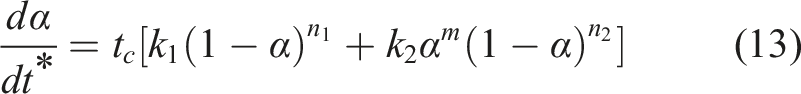

\frac{d α}{d t^{*}} = t_{c} [k_{1} {(1 - α)}^{n_{1}} + k_{2} α^{m} {(1 - α)}^{n_{2}}]

(13)

Parametric study

To explore the effect of the observed spatial variability in HTC on the temperature distribution through the thickness of the laminate, FE simulations were performed. Two metrics were used,

i. The time to reach steady state at the imposed dwell temperature through the thickness. A 1°C margin above was added for robustness

ii. The absolute difference between the temperature of the hottest and coldest nodes at each time

These metrics capture the lag between the prescribed temperature and those in the laminate, and temperature inhomogeneity in the laminate itself. HTCs representing low and high oven values, and an autoclave at 7 bars were considered (Table 2).

Table 2.

Parameters used in the coupled heat transfer and cure kinetics simulations.^25,36

Parameter	Value
Effective laminate density	1580 kgm⁻³
Fibre volume fraction	0.6
Volumetric latent heat	2.12e+8 Jm⁻³
Tool density	8100 kgm⁻³
Tool conductivity	15 Wm⁻¹K⁻¹
Tool specific heat capacity	515 Jkg⁻¹K⁻¹
Part thicknesses	5, 10, 15 mm
HTCs (temperature analysis)	25, 50, 150 Wm⁻²K⁻¹
HTCs (cure analysis)	15–215 Wm⁻²K⁻¹

Further simulations were performed to investigate how the curing process of an epoxy composite laminate was affected by HTC. For completeness the HTC range from Figure 3 was considered, it is noted the extreme values are outliers. While these values reflect the environment within the devices, it is important to note the absence of a vacuum bag which reduces the HTC seen by manufactured parts.

The influence of HTC on the curing process was characterised using three metrics:

i. Cure time, the time for the DOC to exceed 90% through the thickness

ii. Temperature overshoot, the greatest positive difference between the predicted temperature and the 180°C dwell temperature through the thickness

iii. Gel time, the time for the DOC to reach gelation (assumed to be 50% DOC) through the thickness

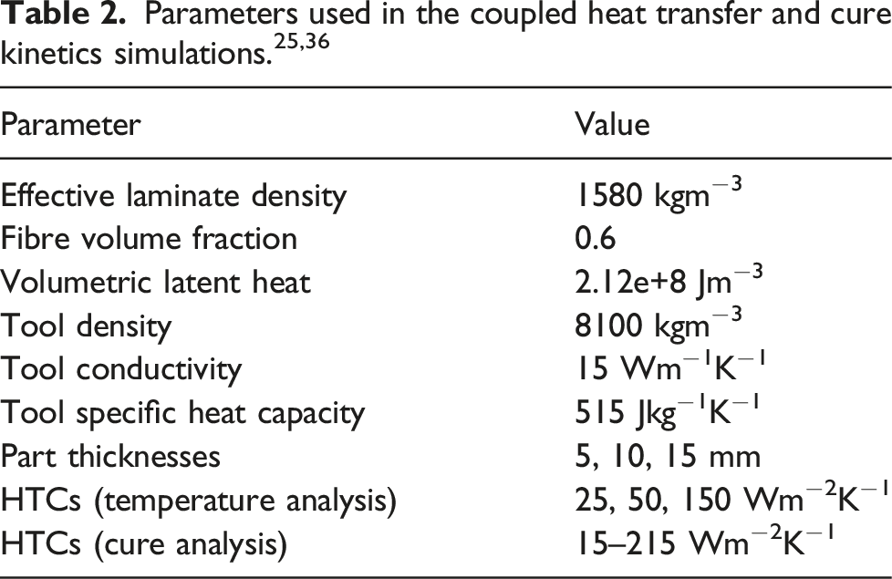
The simulations were performed with the parameters listed in Table 2.

Numerical results

Dimensional analysis

The Biot number in the nondimensionalised boundary conditions indicated the need to model the temperature gradient through the domains. Figure 5 shows Biot number was lowest at the smallest values of HTC and thickness. The value for the laminate never dropped below the 0.1 threshold required to assume lumped capacitance, justifying the need to model the heat transfer within it. The middle plot in Figure 5 shows lumped capacitance could only be assumed in the tool for HTCs less than 150 Wm⁻²K⁻¹, hence for consistency across the analyses, the temperature field in the tool was fully computed in all simulations.

Figure 5.

Variation of laminate (left) and tool (middle) Biot numbers with HTC, and laminate Fourier number with thickness (right). 90% DOC assumed where applicable.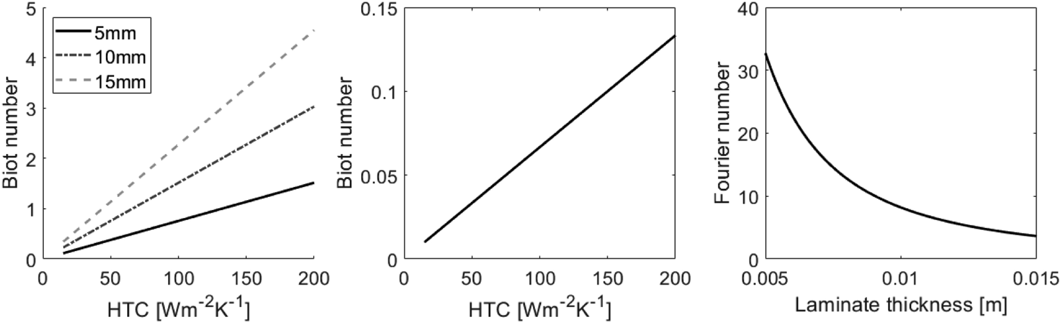

Fourier number gives the ratio of the rate of heat transfer to the rate of heat storage. Fourier number is greater with a thinner part, indicating efficient dissipation of exothermic heat, combating the occurrence of severe temperature overshoots. Owing to the much greater conductivity of invar, the tool Fourier number of 176 far exceeded any of the laminate values shown in Figure 5. The ability of the tool to transfer heat much faster than accumulating it makes it influential in dispersing exothermic heat. Being significantly greater than unity, the Fourier numbers indicate the need to model conduction $(\frac{d^{2} T}{d x^{2}})$ in both domains.

Phase transition number gives the ratio of the exothermic heat to the amount of heat available due to the temperature ramp. Values greater than unity indicate the curing reaction is the dominant form of heating during the ramp, suggesting the occurrence of a highly influential exotherm. In this case, phase transition number was 0.86, below unity, indicating the environment was the primary source of heating, however, its proximity to one indicates the relevance of the exotherm and justified the coupling of the two sub-models.

Effect of HTC on through thickness temperature

Time to reach the prescribed dwell temperature

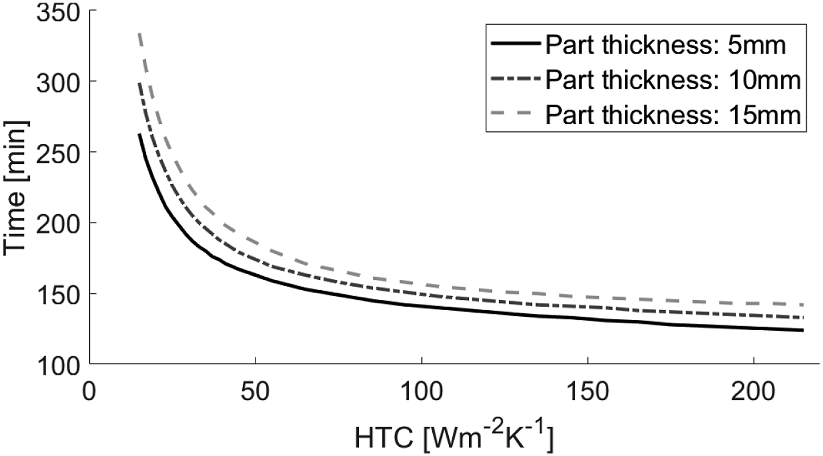
Figure 6 illustrates the effect of HTC on the temperature history in a 10 mm thick laminate. With this thickness, the effect of position in the laminate is negligible compared to the effect of the changes in HTC. The difference between the three sets of curves reflects the non-linearity in Figure 7, a bigger change occurring with the step from 25 Wm⁻²K⁻¹ to 50 Wm⁻²K⁻¹ despite its smaller size. The reduced time with increasing HTC shown in Figure 7 is clearly attributed to the smaller temperature lag with the surroundings during the ramp and the smaller temperature overshoot.

Figure 6.

Air/laminate boundary and central laminate temperatures during the process. For HTCs of 25, 50 and 150 Wm⁻²K⁻¹ with a 10 mm thickness.

Figure 7.

Time to reach dwell temperature over the range of observed HTCs for part thicknesses of 5, 10 and 15 mm.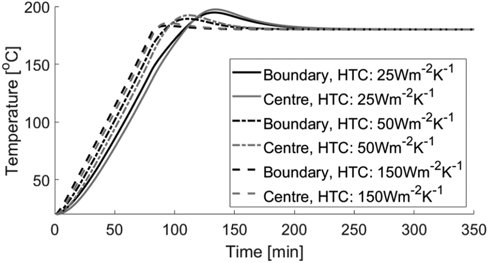

Establishing through thickness temperature homogeneity

Figure 8 shows how the maximum transverse temperature difference changes with time in a 10 mm part. Analogous trends were observed for the other part thicknesses, with values that were scaled in proportion to the thickness, according to the change in Biot number.

Figure 8.

Maximum through thickness temperature difference with time for HTCs of 25, 50 and 150 Wm⁻²K⁻¹ with a part thickness of 10 mm.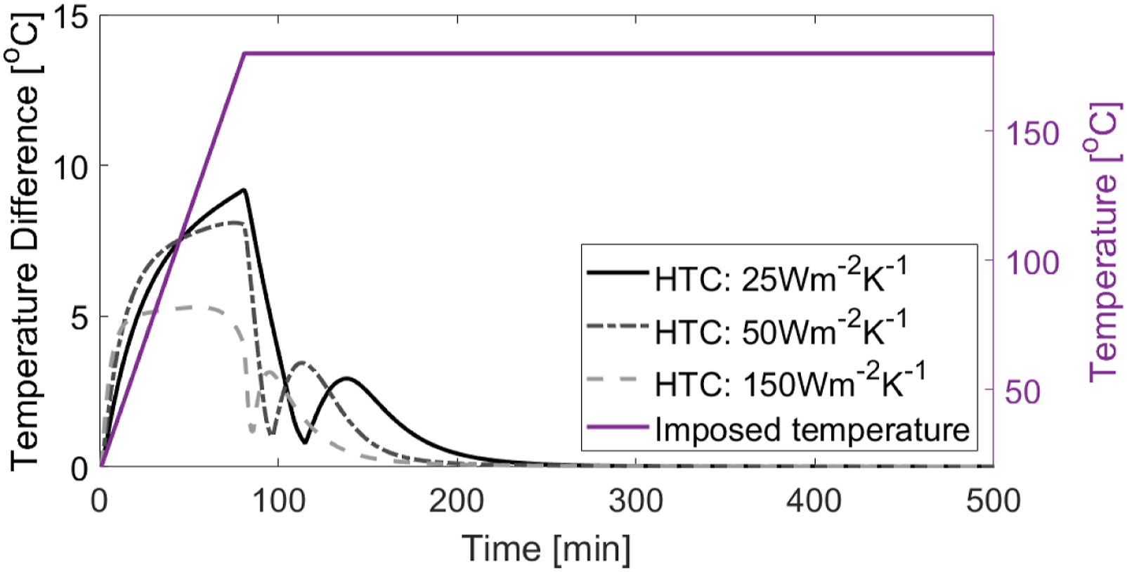

The trends in Figure 8 are reflective of a higher HTC helping to impose the ramp up and mitigate overheating due to the exotherm. The key points can be explained by considering the heat transfer from the two sources of heat, the environment, and the exothermic curing reaction.

The initial heat input is solely from the environment via convective heat transfer, so the air/laminate boundary is initially the hottest point of the laminate, and the centre the coolest. The increasing temperature difference is due to the low transverse conductivity. The temperature difference peaks at the end of the ramp, beyond this point convective heating from the environment becomes less significant.

The minima represent the points at which the location of highest temperature moves from the boundary into the laminate because of the exotherm. The second maxima represent the peak temperature overshoots, the centre of the laminate is hottest and the boundary the coldest.

Effect of HTC on cure through the thickness

Cure time

Cure time as defined above varied in a non-monotonic fashion as HTC increased. Figure 9 illustrates this relationship for the three part thicknesses considered. Initially cure time decreased with increasing HTC, taking a minimum value between 25 and 35 Wm⁻²K⁻¹, before increasing.

Figure 9.

Cure time approximated for the geometry over the range of observed HTCs for part thicknesses of 5, 10 and 15 mm. The cure time if the matter followed the cycle is 178 min. The error bars mark 95% confidence intervals (CI) for the specific case of HTC measured in the vessels.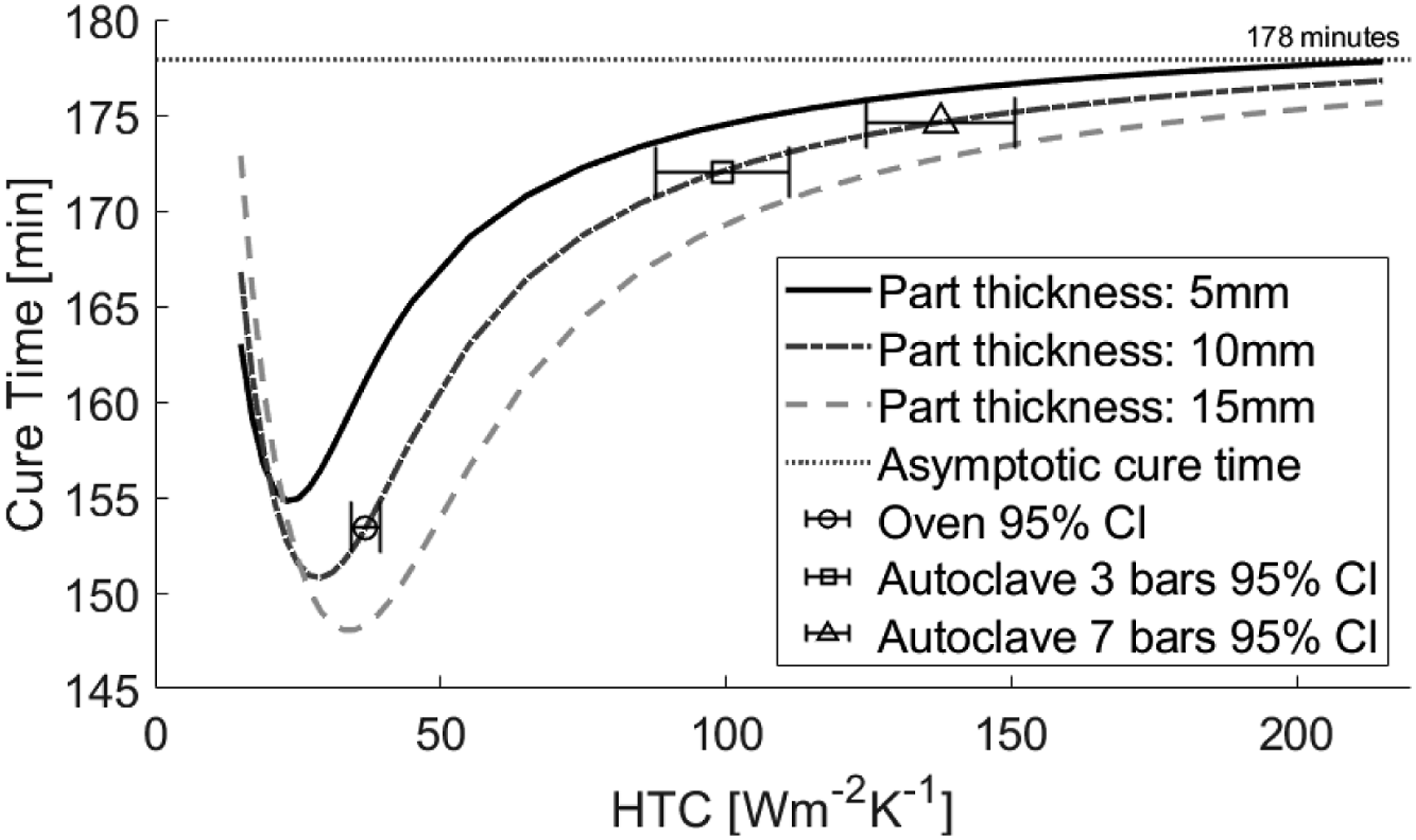

This relationship can be expressed by considering Figure 6. At HTCs below the minima the resistance at the boundary is too great for effective heating. At HTCs above the minima the low resistance at the boundary reduces the influence of exothermic heat. The minima represent a balance of the two effects; however, it is unlikely to be optimal due to overheating.

The error bars represent 95% confidence intervals for the HTCs measured in the three types of vessels, assuming normal distributions. To maximise generality, measurements from the ovens and autoclaves were grouped together, as in Figure 3. They illustrate the range of cure times possible with a 10 mm thick part.

The lower minimum with increasing part thickness can be attributed to greater temperature overshoot (Figure 10). The offsets in time are due to the higher Biot numbers indicated in Figure 5.

Figure 10.

Temperature overshoot approximated for the geometry over the range of observed HTCs for part thicknesses of 5, 10 and 15 mm. The error bars mark 95% confidence intervals (CI) for HTC measured in the vessels.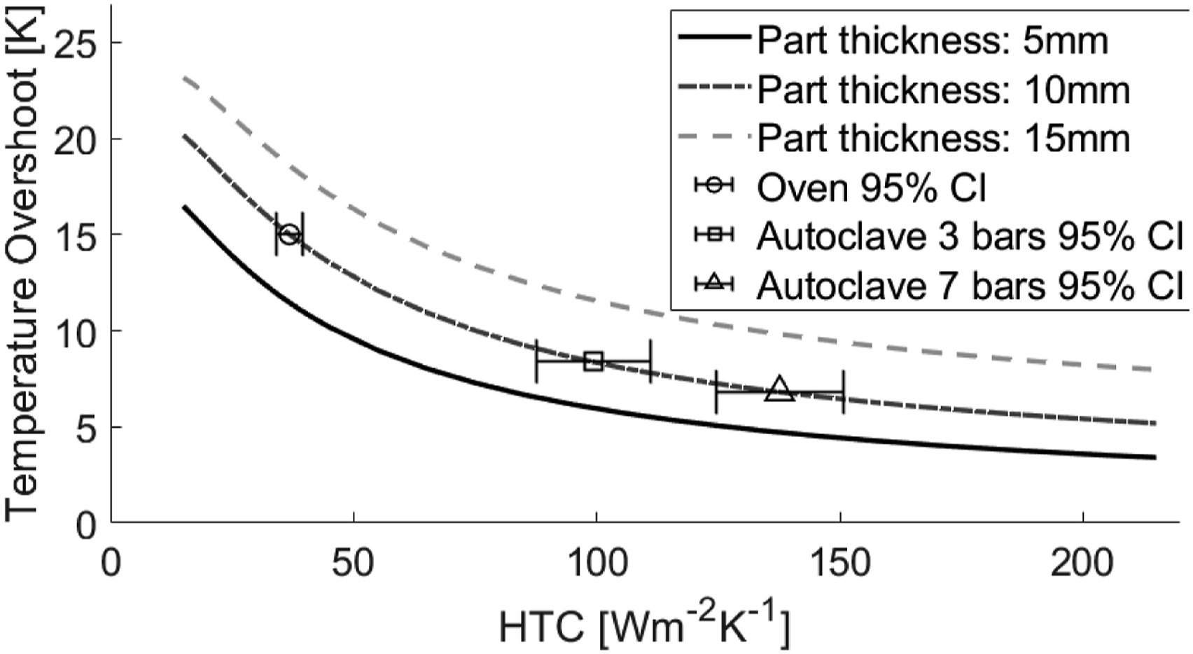

Cure time depends on the node where cure occurs slowest. As Biot number increases the exothermic heating at the centre has less influence on the boundary. Hence the convergence of cure times beyond the minima.

Temperature overshoot

The curves in Figure 10 are highly similar, the thickness increases mostly causing a translation. The size of the translation is clearly non-linear, the increasing difference reflecting the change in Fourier number and the Arrhenius temperature dependence of the cure kinetics.²⁵ The same 95% confidence interval error bars as in Figure 9 have been applied to mark the possible overshoot variation in a 10 mm thick part.

As Biot number increases, the temperature distribution through the thickness becomes less uniform, the resulting temperature gradient combined with the lower boundary resistance increases the dispersion of exothermic heat in accordance with Fourier and Darboux.²⁹

Gel time

Gel time as defined above decreases with increasing HTC as shown in Figure 11. As with cure time, at high values of HTC, the gel times for the different thicknesses converge. Again, this is attributed to the increasing dominance of conductive resistance making the reaction at the boundary increasingly dependent on the environment and less dependent on the exothermal heating centred at the middle of the part.

Figure 11.

Gel time approximated for the geometry over the range of observed HTCs for part thicknesses of 5, 10 and 15 mm. The gel time if the matter followed the cycle is 93 min.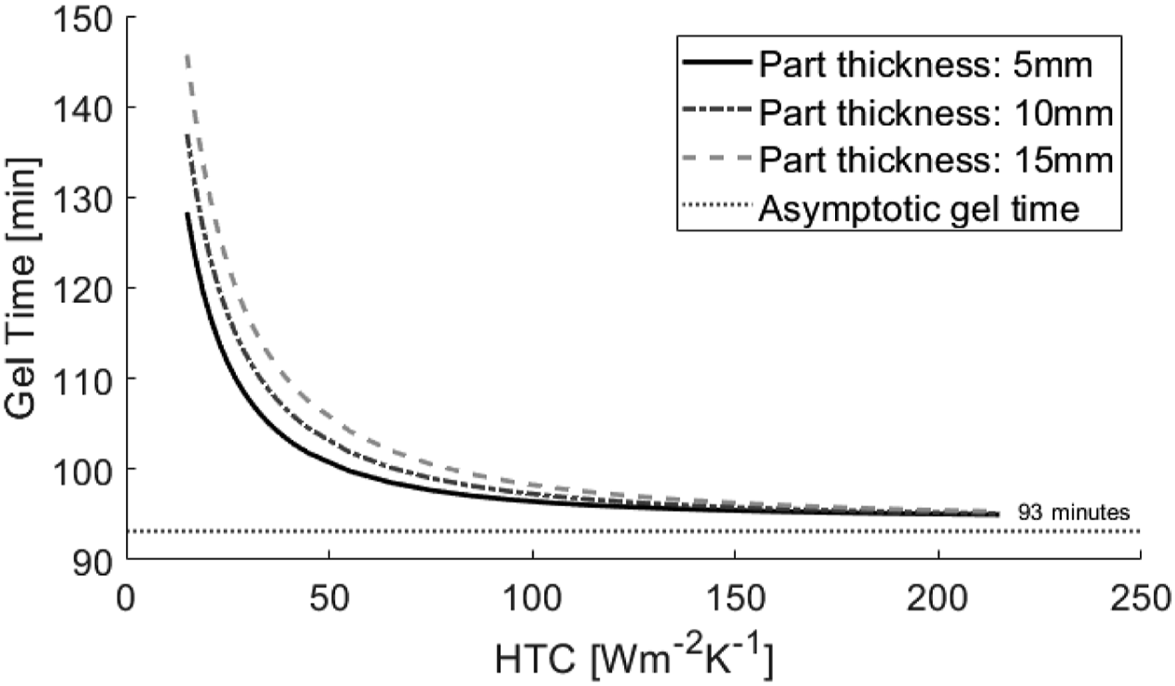

Unlike cure time, gel time decreases monotonically with increasing HTC. The difference is made clear by Figure 6, for the HTCs measured, the gel time (when DOC reaches 0.5) elapsed before the temperature overshoot (occurring at DOC of around 0.8). Therefore, the change in gel time due to HTC is only affected by the effective ramp rate in the material which increases with HTC, and not exotherm effects.

Discussion

Efficiency-quality trade-off

For this combination of configuration and temperature history, none of the ovens have sufficient HTCs (>45 Wm⁻²K⁻¹) throughout to prevent temperature overshoots exceeding 10°C for any of the part thicknesses studied here. With the non-linear increase of temperature overshoot with part thickness noted previously, although the 5 mm part can be safely cured in the autoclaves, only autoclave 1 at 7 bars is suitable for the 15 mm part. This level of overshoot is significant for M21 as phase changes have been reported above these temperatures.²⁵

The flattening of the temperature overshoot-HTC curve in Figure 10 highlights the limitations of the curing environment for reducing temperature overshoot. The cure cycle used is representative of one typically used with thinner parts, a relatively high ramp rate (2°Cmin⁻¹) with no pre-dwell. It is clearly not suitable for curing M21 composite parts in oven environments. To reduce the rate of exothermic heating, features such as pre-dwells and slower temperature ramps must be added. However, these features can significantly reduce processing efficiency, hence by operating in autoclave HTC regimes, greater part thicknesses can be processed before such inefficiencies are necessary.

Effect of spatial heat transfer coefficient variability

The error bars in Figures 9 and 10 were used to consider how the spatial variability in HTC could propagate through the curing process, using cure time and temperature overshoot for a 10 mm thick part as metrics. The ranges of cure time and temperature overshoot corresponding to the bounds of the error bars for the three types of vessels are shown in Table 3.

Table 3.

Cure time and temperature overshoot corresponding to the bounds of 95% confidence intervals for HTC in each vessel type assuming a normal distribution.

	Ovens	Autoclaves 3 bars	Autoclaves 7 bars
Cure time (min)	152.1, 154.8	170.7, 173.0	173.9, 175.2
Temperature overshoot (°C)	14.5, 15.5	7.8, 9.1	6.4, 7.3

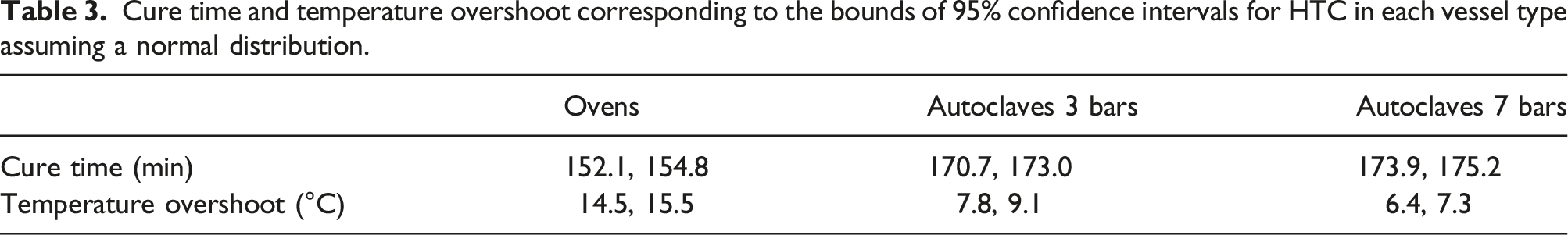
With a mean HTC of 37 Wm⁻²K⁻¹ the oven confidence interval straddles a steep section of the cure time-HTC curve (Figure 9). Despite this, the small spatial variability of HTC in the ovens resulted in a narrow range of cure time values. In contrast, the respective means of 99 Wm⁻²K⁻¹ and 138 Wm⁻²K⁻¹ for the autoclaves at 3 and 7 bars were on much shallower sections of the curve. However, due to the greater spatial variability in these vessels, this advantage from the higher HTCs was largely offset. Consequently, the range of cure times predicted for the three types of vessels were similar, the closest ranges being for the ovens and autoclaves at 3 bars, with the autoclaves at 7 bars having the narrowest range. These results show the much greater robustness to HTC variability at higher HTC values.

The more comparable gradients at oven and autoclave HTCs in Figure 10 meant the lower spatial variability in the ovens produced a range of cure times practically indistinguishable from the autoclaves. The oven range was narrower than predicted for the autoclaves at 3 bars and essentially the same as the autoclaves at 7 bars. Hence, for practical purposes, the predictability of overshoot is consistent among the vessels.

In terms of the overshoot values themselves, even the lower bound of the oven was excessive. Whereas both autoclaves had upper bounds below the 10°C threshold imposed by the material. This suggests only the autoclaves were capable of curing the 10 mm thick part reliably.

The monotonic nature of Figure 10 results in a simpler interpretation for temperature overshoot, where higher HTC values result in a lower mean and greater robustness to HTC variability. Furthermore, the rate of improvement diminishes at a slower rate as HTC increases compared to cure time.

Conclusion

The curing of composite laminates on a mould, in a vessel (oven or autoclave) is driven by heat transfer. Classically, heat transfer within the part is modelled using a convective heat transfer coefficient (HTC) at the boundaries.

In this study, experimental HTC data from a range of oven sizes, including two large pre-production ovens, was compared to autoclave data. Statistical analysis was conducted to investigate the spatial variability of HTC within the vessels. A coupled Finite Element model was used to propagate the measured uncertainty through the curing reaction to predict the effects on final part quality. The effects were assessed using five indicators, two to consider temperature and three for the cure reaction.

The temperature indicators showed that the temperature history was more successfully imposed with the higher HTCs measured in the autoclaves. This is realised with less temperature lag during the ramp-up and smaller temperature overshoot during exothermic reaction.

The key result was that despite the greater robustness to spatial HTC variability at autoclave HTCs, the larger variability in the autoclave HTC data resulted in similar robustness of the cure reaction indicators across all vessel types.

This study considered a single cure cycle, one recommended for laminate thicknesses of less than 15 mm.²⁸ Future work could consider the effect of using different cure cycles, for example with different ramp rates and a pre-dwell. These cure cycle parameters could then be optimised for a given combination of vessel and part thickness.

Footnotes

Declaration of conflicting interests

The author(s) declared no potential conflicts of interest with respect to the research, authorship, and/or publication of this article.

Funding

The author(s) disclosed receipt of the following financial support for the research, authorship, and/or publication of this article: This work was supported by the EPSRC Future Composites Manufacturing Research Hub under Grant EP/P006701/1. Data collection was supported by Jason Mareo, Stuart Skyes, and Callum Heath at the National Composites Centre through a RCUK Catapult Researchers in Residence award EP/R513568/1.

Data availability

All underlying data to support the conclusions are provided within this paper.

ORCID iDs

Arthur Levy

James Kratz

Appendix

References

Advani

Hsiao

K-T

. Manufacturing techniques for polymer matrix composites (PMCs). Cambridge: Woodhead Publishing Limited, 2012.

Agius

Magniez

Fox

. Cure behaviour and void development within rapidly cured out-of-autoclave composites. Compos B: Eng 2013; 47: 230–237.

Ghamlouch

. Analysis of convective transfer around simple molds inside a model autoclave. Doctoral dissertation. Université de Nantes, 2018.

Kluge

Lundström

Ljung

A-L

, et al. An experimental study of temperature distribution in an autoclave. J Reinf Plast 2016; 35: 566–578.

Wang

Zhang

Xie

, et al. Correlated rules between complex structure of composite components and manufacturing defects in autoclave molding technology. J Reinf Plast Compos 2009; 28: 2791–2803.

Slesinger

Shimizu

Arafath

, et al. Heat transfer coefficient distribution inside an autoclave. In: 17th International Conference on Composite Material ICCM, Edinburgh, UK, 2009, IOM Communications.

Bohne

Frerich

Jendrny

, et al. Simulation and validation of air flow and heat transfer in an autoclave process for definition of thermal boundary conditions during curing of composite parts. J Compos Mater 2018; 52: 1677–1687.

Kakac

Yener

Pramuanjaroenkij

. Convective heat transfer. Boca Raton: CRC press. 1995.

Zhu

Frerich

Herrmann

. CFD modeling and validation of heat transfer inside an autoclave based on a mesh independency study. J Compos Mater 2021; 55: 2469–2487.

10.

Zobeiry

Forghani

, et al. Multiscale characterization and representation of composite materials during processing. Philos Trans R Soc A: Math Phys Eng Sci 2016; 374: 20150278.

11.

Weber

Arent

J-C

Münch

, et al. A fast method for the generation of boundary conditions for thermal autoclave simulation. Compos A: Appl Sci 2016; 88: 216–225.

12.

Campbell

Jr . Manufacturing processes for advanced composites. Oxford: Elsevier, 2004.

13.

Johnston

. An integrated model of the development of process-induced deformation in autoclave processing of composite structures. Doctoral dissertation. University of British Columbia, 1997.

14.

Dodiuk

. Handbook of thermoset plastics. Norwich, NY: William Andrew, 2022.

15.

Wang

, et al. Monitoring the gelation and effective chemical shrinkage of composite curing process with a novel FBG approach. Compos Struct 2017; 176: 187–194.

16.

Guo

. Thermosets: structure, properties, and applications. Amsterdam: Woodhead Publishing, 2018.

17.

Pusatcioglu

Hassler

Fricke

, et al. Effect of temperature gradients on cure and stress gradients in thick thermoset castings. J Appl Polym Sci 1980; 25: 381–393.

18.

Hilton

. Effects of thermo-mechanical properties of composites on viscosity, temperature and degree of cure in thick thermosetting composite laminates during curing process. J Compos Mater 1998; 32: 600–622.

19.

Loos

Springer

. Curing of epoxy matrix composites. J Compos Mater 1983; 17: 135–169.

20.

Ostrogorsky

. Simple explicit equations for transient heat conduction in finite solids. 2009.

21.

Lienhard

John

. A heat transfer textbook. Cambridge, MA: Phlogiston Press, 2020.

22.

Nam

Lee

Kim

, et al. Experimental study on the emissivity of stainless steel. 2001.

23.

Omega Engineering I . The infrared temperature handbook. Omega Engineering, Incorporated, 1994.

24.

Slesinger

. Thermal modeling validation techniques for thermoset polymer matrix composites. University of British Columbia, 2010.

25.

Mesogitis

Kratz

Skordos

. Heat transfer simulation of the cure of thermoplastic particle interleaf carbon fibre epoxy prepregs. J Compos Mater 2019; 53: 2053–2064.

26.

Kamal

Sourour

. Kinetics and thermal characterization of thermoset cure. J Polym Eng Sci 1973; 13: 59–64.

27.

Guo

Z-S

Zhang

. Temperature field of thick thermoset composite laminates during cure process. Compos Sci Technol 2005; 65: 517–523.

28.

HexPly M21 product data sheet. In: HEXCEL (ed), 2020.

29.

Fourier

JBJ

Darboux

. Théorie analytique de la chaleur. Paris: Didot, 1822.

30.

Lewis

. Mechanical engineering handbook In: Kreith

(ed) Boca Raton: CRC Press LLC, 1999.

31.

Hilpert

. Heat transfer from cylinders. Forsch Geb Ingenieurwes 1933; 4: 215–224.

32.

Raznjevic

. Handbook of thermodynamic tables and charts. Washington DC: Hemisphere Publication Corporation 1976.

33.

Kothandaraman

. Fundamentals of heat and mass transfer. 3rd ed. New Delhi: New Age International, 2006.

34.

Dixon

. The shock absorber handbook. 2nd ed. Chichester, England: John Wiley, 2007.

35.

Ziegler

. The multiple meanings of the Stefan-number (and relatives) in refrigeration. Int J Refrig 2010; 33: 1343–1349.

36.

Invar-Nickel Iron Alloy, https://www.azom.com/properties.aspx?ArticleID=515

Effects of heat transfer coefficient variations on composite curing

Abstract

Keywords

Introduction

Experimental mapping of HTC in ovens and autoclaves

Methods

Temperature measurements

Heat transfer coefficient estimation

Validating the lumped mass assumption

Checking for negligible radiative heat transfer

Experimental results

HTC variability between the vessels

Spatial HTC variability within the vessels

Numerical methods and results

Numerical modelling

Numerical implementation

Dimensional analysis

Parametric study

Numerical results

Dimensional analysis

Effect of HTC on through thickness temperature

Time to reach the prescribed dwell temperature

Establishing through thickness temperature homogeneity

Effect of HTC on cure through the thickness

Cure time

Temperature overshoot

Gel time

Discussion

Efficiency-quality trade-off

Effect of spatial heat transfer coefficient variability

Conclusion

Footnotes

Declaration of conflicting interests

Funding

Data availability

ORCID iDs

Appendix

References