Sage Journals: Discover world-class research

Abstract

The effect of matrix and fibre cracks on the static strength and stiffness of uni-directional plies and cross-ply laminates under tensile loads was examined with the goal of understanding the main damage mechanisms. The size of matrix cracks emanating from cracked fibres was determined and found to be in excellent agreement with test results. This was used to predict static tensile failure of uni-directional laminates and was shown to be in good to excellent agreement with test results for six different materials. The approach was extended to fatigue loading by determining the number of cycles for the plastic zone ahead of a matrix crack tip to fail. It was combined with an approach to quantify the effect of matrix cracks under any in-plane loading previously developed by the authors to predict changes in laminate stiffness as a function of cycles. Comparisons with test results showed good to excellent agreement between predicted and measured laminate stiffness as a function of fatigue cycles.

Keywords

Fiber cracks matrix cracks ply strength stiffness degradation fatigue damage

Introduction

Understanding the mechanisms of damage creation and evolution during fatigue loading of composite structures requires modelling the basic types of damage, fibre cracks, matrix cracks and delaminations. Over the years, attempts in that direction ranged from curve fits and phenomenological models relating fatigue performance to a macroscopic property such as residual strength or stiffness, to detailed simulations of the different types of damage. Very good overviews of these areas were presented by Degrieck and van Paepegem¹ and Passipoularidis and Brønsted.² Phenomenological models^3,4 tend to be simpler and easier to implement but do not explicitly model damage creation and evolution. A number of tests is needed to determine model parameters and the range of applicability of the models may be limited. The approaches simulating damage in detail are of primary interest here because they attempt to relate physical phenomena with damage creation. In earlier work, Talreja^5,6 modelled inter-laminar and intra-laminar cracks using continuum mechanics. Stiffness degradation was a function of the amount of damage present. Tests were needed to link residual stiffness to crack density.

Deviating from more traditional approaches which model stiffness degradation, Aboudi et al.⁷ suggested that the Poisson’s ratio is a good indicator of the state of damage in a cross-ply laminate. They solved the elasticity equations in a three dimensional context using a repeating unit cell. Van Paepegem et al.⁸ also used the Poisson’s ratio to indirectly monitor evolution of fatigue damage.

A two-dimensional model was used by Berthelot and Le Corre⁹ to model transverse matrix cracks in cross-ply laminates under static loads. Under fatigue loading, when the transverse cracks do not extend to the full width of the specimen, they combined their two-dimensional model with finite element analysis to create a quasi-three-dimensional model for matrix crack evolution. Montesano et al.¹⁰ combined finite element modelling with a statistical model for the variation of the critical strain energy release rate to predict matrix crack evolution and stiffness degradation for laminates under multi-axial loading.

Shokrieh and Lessard,¹¹ combined finite element-based stress analysis with models for material degradation to set up a progressive damage model for laminates under fatigue loading. Ladeveze and Le Dantec,¹² used damage variables at the ply level to quantify matrix micro-cracking and fibre-matrix debonding. Maimí et al.,¹³ also used damage variables to determine intralaminar failure mechanisms.

More recently, Breite et al.,¹⁴ evaluated six models for the tensile failure of uni-directional composites. They found that the load distribution in the vicinity of broken fibres and subsequent crack creation in them plays a big role making it hard to obtain accurate predictions for the ultimate strain and stress of a ply. Bonora et al.¹⁵ used Talreja’s continuum mechanics model^5,6 to relate stiffness degradation to density of matrix cracks in the 90° plies. They related crack density to applied cycles, maximum cyclic stress, specimen geometry and certain constants, one of which is a function of applied load level. As alluded to, in much of previous work, knowledge of crack density is a necessary intermediate step in predicting residual stiffness of a laminate under fatigue loading. Mohammadi and Pakdel¹⁶ used a variational approach and a Paris-type growth law to predict crack density. The two parameters in the growth law were determined from tests on two different laminates.

Depending on the approach used, previous work has focused mostly on phenomenological, semi-empirical, and simulation models. Accordingly, some methods depend on curve fitting, extensive testing, or indirectly determined parameters which allow modelling of damage creation and evolution. As a result, the applicability and accuracy of many of these methods as well as the computational cost of the more elaborate ones point to the need for a generalized approach which accounts for the major damage mechanisms, does not rely on extensive testing to obtain model parameters and accurately predicts static and fatigue behaviour both in terms of strength an stiffness.

The present work aims at providing a general analytical approach for predicting the static and fatigue strength and stiffness of uni-directional plies without the need for additional testing or curve fitting. In addition, it is very efficient and is able to capture the basic physics of damage formation and evolution under static and fatigue loads. It models the creation and evolution of fibre cracks in the 0 plies and fibre/matrix interface or transverse matrix cracks in the 90 plies. At the same time it addresses failure mechanisms and their interactions under static loads allowing accurate determination of uni-directional ply strength using individual fibre and matrix properties. One of its added features is the ability to determine under what conditions matrix cracks will develop parallel or perpendicular to the fibres. The approach is also applied to fatigue loading where it is combined with a model to predict ply crack evolution in order to accurately determine cycles to failure and stiffness reduction as a function of cycles.

Approach

Strength and stiffness of a 0° unidirectional tape ply

Stress field around fibre crack

A 0° ply under uni-axial load will develop cracks in the fibres. The location of these cracks is, at the beginning, random. For a given applied tensile strain, some fibres may develop multiple cracks which, at lower strains, are not evenly spaced, while other fibres may remain intact. The case of a cracked fibre in a ply is shown in Figure 1. Depending on the situation, as the applied strain increases, in addition to more fibre cracks appearing in various fibres, some of the cracks transition to fibre/matrix interface cracks or matrix radial inter-fibre cracks. These are also manifested during fatigue loading.^17,18 Which type of crack will appear in a particular situation depends mostly on the fibre volume fraction as will be shown later.

Figure 1.

Fibre crack transitioning to fibre/matrix interface or matrix inter-fibre radial crack.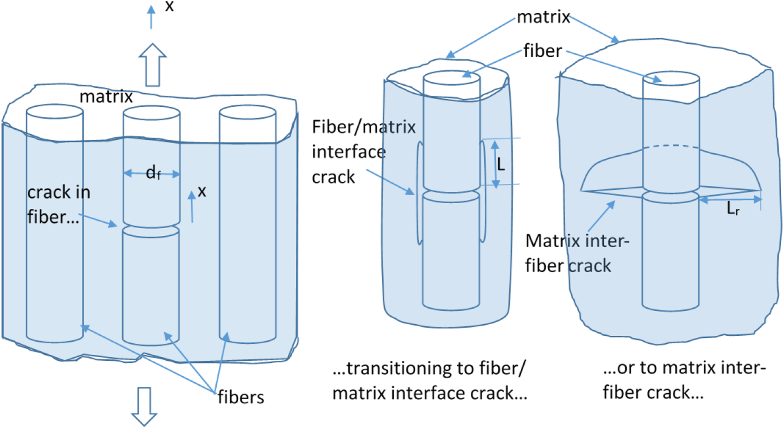

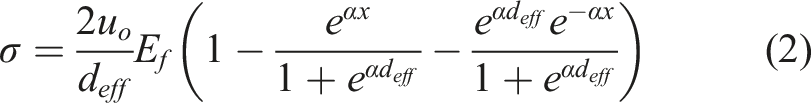
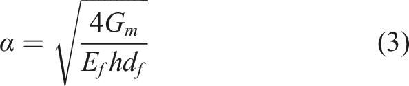
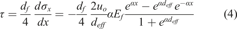
When a fibre first cracks and before the matrix fails locally, the load in the fibre shears into the matrix around the fibre crack and the fibre can still carry load effectively. The (shear lag) distance on either side of the fibre crack over which the stress in the fibre goes from 0 at the crack tip to the far-field applied stress, is denoted by the ratio d_eff/2. The matrix near the cracked fibre is assumed to be in pure shear. By balancing an element of length dx along the cracked fibre and recovering uniform axial extension at the far field, the governing equation is obtained:

\frac{d^{2} σ}{d x^{2}} - \frac{4 G_{m}}{E_{f} h d_{f}} σ = - \frac{8 G_{m} u_{o}}{h d_{f} d_{e f f}}

(1)

where σ is the axial stress in the fibre, u_o is the applied displacement on fibre and matrix at d_eff/2, G_m is the matrix shear modulus, E_f is the fibre longitudinal Young’s modulus, h is the radial distance from the cracked fibre over which the matrix is in pure shear and d_f is the fibre diameter. These quantities are visualized in Figures 2 and 4 below. Many authors have proposed different versions of equation (1) in the past [for example].^19–21 More recently, the work by Sørensen²² for single fibres in a matrix should be noted because it included the effect of friction at the fibre/matrix interface. The main differences in the present formulation are in the non-homogenous term on the right hand side of equation (1), which is based on fibre strains, and in the use of the length scale h (see below) which represents the portion of the matrix under pure shear. It should also be noted that, once a (radial) matrix crack appears, the matrix is no longer assumed to be under pure shear and the complete three-dimensional state of stress in the matrix is accounted for through the use of the Nied-Erdogan solution²³ (see equation (24)). Equation (1) is solved with boundary conditions of σ = 0 at x = 0 (crack location) and u = u_o at x = d_eff/2 where the far-field stress in the fibre is recovered. The solution is:

σ = \frac{2 u_{o}}{d_{e f f}} E_{f} (1 - \frac{e^{α x}}{1 + e^{α d_{e f f}}} - \frac{e^{α d_{e f f}} e^{- α x}}{1 + e^{α d_{e f f}}})

(2)

where,

α = \sqrt{\frac{4 G_{m}}{E_{f} h d_{f}}}

(3)

Figure 2.

Distance along which shear stress at the fibre/matrix interface exceeds matrix shear strength.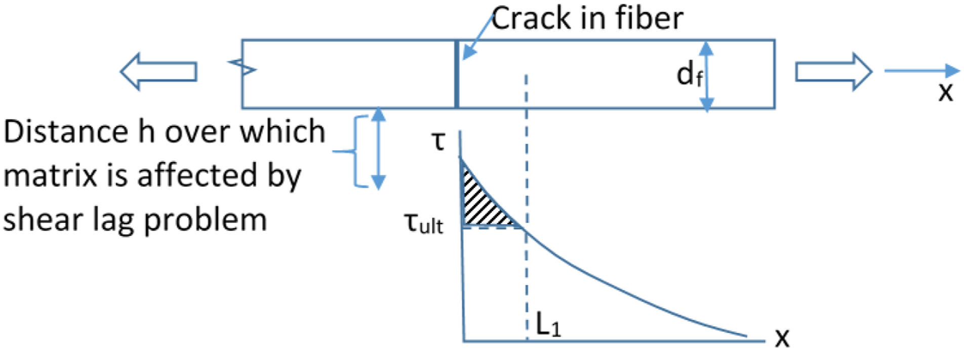

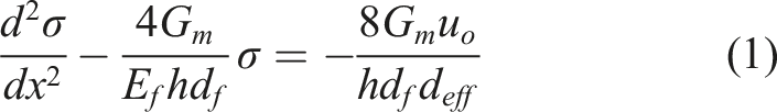
The shear stress τ in the matrix is obtained from equilibrium:

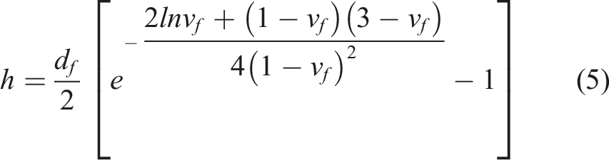
τ = \frac{d_{f}}{4} \frac{d σ_{x}}{d x} = - \frac{d_{f}}{4} \frac{2 u_{o}}{d_{e f f}} {α E}_{f} \frac{e^{α x} - e^{α d_{e f f}} e^{- α x}}{1 + e^{α d_{e f f}}}

(4)

For the radial distance h from the center of the cracked fibre over which the matrix is in pure shear the expression by Budiansky et al.²⁴ is used:

h = \frac{d_{f}}{2} [e^{- \frac{2 \ln v_{f} + (1 - v_{f}) (3 - v_{f})}{4 {(1 - v_{f})}^{2}}} - 1]

(5)

where v_f is the fibre volume fraction. The effective length of fibre d_eff can now be obtained by finding the length d_eff/2 needed for the stress to reach 99% of its nominal uncracked fibre value. Using ε_aE_f as the stress in the uncracked fibre with ε_a the applied strain, equation (2) gives:

1 - 2 e^{\frac{α d_{e f f}}{2}} + e^{α d_{e f f}} = 0.99 + 0.99 e^{α d_{e f f}}

(6)

where the fact that ε_a = 2u_o/d_eff was used. Equation (6) is quadratic in

e^{α d_{e f f} / 2}

. Solving for d_eff, leads to:

d_{e f f} = \frac{10.5966}{α}

(7)

Fibre/matrix interface crack

If the fibre/matrix interface bond is not sufficiently strong, the shear stress from equation (4) will lead to cracking of the fibre/matrix interface. This is shown in the second image of Figure 1. At this point, the matrix shear stress-strain curve is assumed to be linear to failure and to have the same ultimate strength as obtained by tests and with the same area under the curve as the non-linear shear stress-strain curve. This is an approximation and a limitation to be relaxed during further future model development. If τ_ult is the shear failure strength of the matrix, for sufficiently high applied strain, there will be a length L₁ measured from the crack location, parallel to the fibre over which the shear stress in the matrix exceeds τ_ult. This is shown in Figure 2. The length L₁ is found by setting τ = τ_ult in equation (4).

L_{1} = \frac{1}{α} \ln [\frac{- H + \sqrt{H^{2} + 4 e^{α d_{e f f}}}}{2}]

(8)

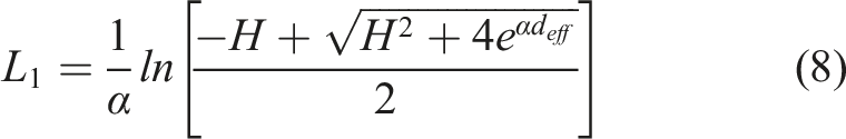
With,

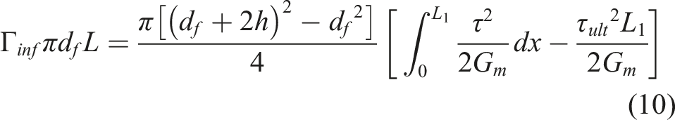
H = \frac{τ_{u l t} 4 (1 + e^{α d_{e f f}})}{d_{f} α \frac{2 u_{o}}{d_{e f f}} E_{f}}

(9)

A measure of the energy that would be released if such a longitudinal crack were created can be obtained by calculating the energy corresponding to shear stress in excess of τ_ult over a length L₁. Assuming that the matrix at the fibre/matrix interface is mostly in shear, failure of the interface would occur when the shear stress in the matrix exceeds τ_ult. The region along the fibre over which this ultimate shear strength would be exceeded if there were no failure corresponds to the size of a longitudinal crack, if dynamic effects are excluded. This approach has been applied successfully by Huo et al.²⁵ to determine delamination size of laminates under static indentation and by Esrail and Kassapoglou²⁶ to determine delamination sizes of laminates under low speed impact damage. Denoting by Γ_inf the fracture energy per unit area of interface crack created and by L the length of interface crack resulting by this released energy, the energy to create a crack can be set equal to that released due to the shear stress exceeding its ultimate value. This gives:

Γ_{\inf} π d_{f} L = \frac{π [{(d_{f} + 2 h)}^{2} - {d_{f}}^{2}]}{4} [\int_{0}^{L_{1}} \frac{τ^{2}}{2 G_{m}} d x - \frac{{τ_{u l t}}^{2} L_{1}}{2 G_{m}}]

(10)

Using equation (4) to substitute for τ and solving for the interface crack length L gives:

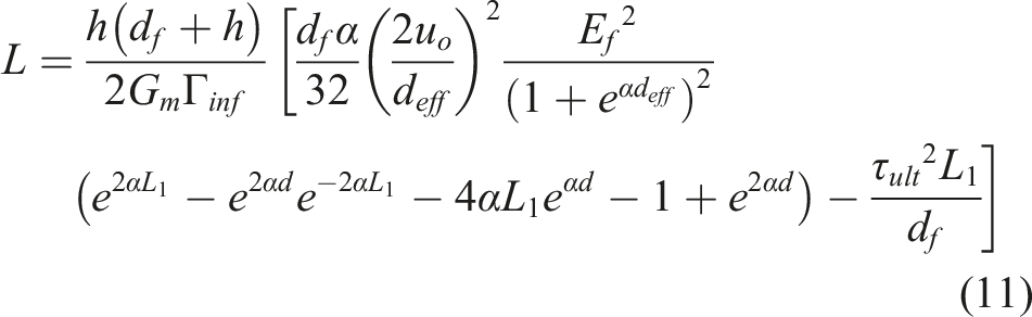
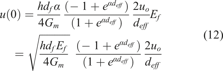
L = \frac{h (d_{f} + h)}{2 G_{m} Γ_{\inf}} [\frac{d_{f} α}{32} {(\frac{2 u_{o}}{d_{e f f}})}^{2} \frac{{E_{f}}^{2}}{{(1 + e^{α d_{e f f}})}^{2}} (e^{2 α L_{1}} - e^{2 α d} e^{- 2 α L_{1}} - 4 α L_{1} e^{α d} - 1 + e^{2 α d}) - \frac{{τ_{u l t}}^{2} L_{1}}{d_{f}}]

(11)

Equation (11) gives an estimate of the length of the fibre/matrix interface crack. The accuracy of this equation is evaluated by comparing its predictions to measurements done by Kim and Nairn²⁷ for individual AS4 and E-glass fibres embedded in epoxy. In that work, the length was measured under load and included the fibre crack opening. The latter can be estimated by combining equations (2) and (4) to calculate the displacement u (0) (at x = 0 in Figure 1):

u (0) = \frac{h d_{f} α}{4 G_{m}} \frac{(- 1 + e^{α d_{e f f}})}{(1 + e^{α d_{e f f}})} \frac{2 u_{o}}{d_{e f f}} E_{f} = \sqrt{\frac{h d_{f} E_{f}}{4 G_{m}}} \frac{(- 1 + e^{α d_{e f f}})}{(1 + e^{α d_{e f f}})} \frac{2 u_{o}}{d_{e f f}}

(12)

In comparing with the results by Kim and Nairn in ref. 27 the results of equations (10) and (12) are multiplied by 2 to account for the interface crack extending to both sides of the fibre crack (above and below the crack in Figure 1). Also, for high applied strains, exceeding 0.0175 for AS4 and 0.025 for E-glass, the crack spacing is less than d_eff. In such cases, the measured crack spacing from Figure 9 in ref. 27 was used. For Γ_inf, the measured values of 220 J/m² for AS4 and 105 J/m² for E-glass from²⁷ were used here. Any needed material properties were obtained from²⁷ and Table 1 below. Comparison of the predictions of the present method to results in Figures 23 and 24 in ref. 27 are shown in Figure 3. There is significant scatter in the test data but for both materials, very good agreement is observed.

Table 1.

Material properties used to predict strain and stress to failure for four different uni-directional materials (all data from²⁸ unless otherwise noted).

Property	AS4/3501-6	IM7/8552	G40-800/5260	Glass/LY556	34-700/736LT⁽³⁾	T700SC-12/SR8500-KTA315⁽³⁾
Fibre diameter d_f (μm)	7	4.5	8	11	6.5	6.8
Fibre Young’s modulus, E_f (GPa)	231	276	290	74	234	230
Fibre mean strain to failure, ε_fm	0.01515	0.0187	0.0202	0.02905	0.01691	0.01666
Fibre std dev, of strain distr, s_f	0.00237⁽¹⁾	0.00293⁽¹⁾	0.00316⁽¹⁾	0.00617⁽²⁾	0.00380⁽¹⁾	0.00453⁽¹⁾
Matrix shear modulus, G_m (GPa)	1.567	1.478	1.28	1.24	0.904	0.989
Matrix Young’s modulus, E_m, (GPa)	4.2	4.08	3.45	3.35	3.15	3.36
Matrix Poisson’s ratio ν	0.34	0.38	0.35	0.35	0.39	0.42
Matrix ultimate shear strength τ_ult (MPa)	50	57	57	54	60.4	63.3
Mode I critical energy release rate G_Icm = Γ_inf (J/m²)	220	200	240	165	220⁽⁴⁾	220⁽⁴⁾

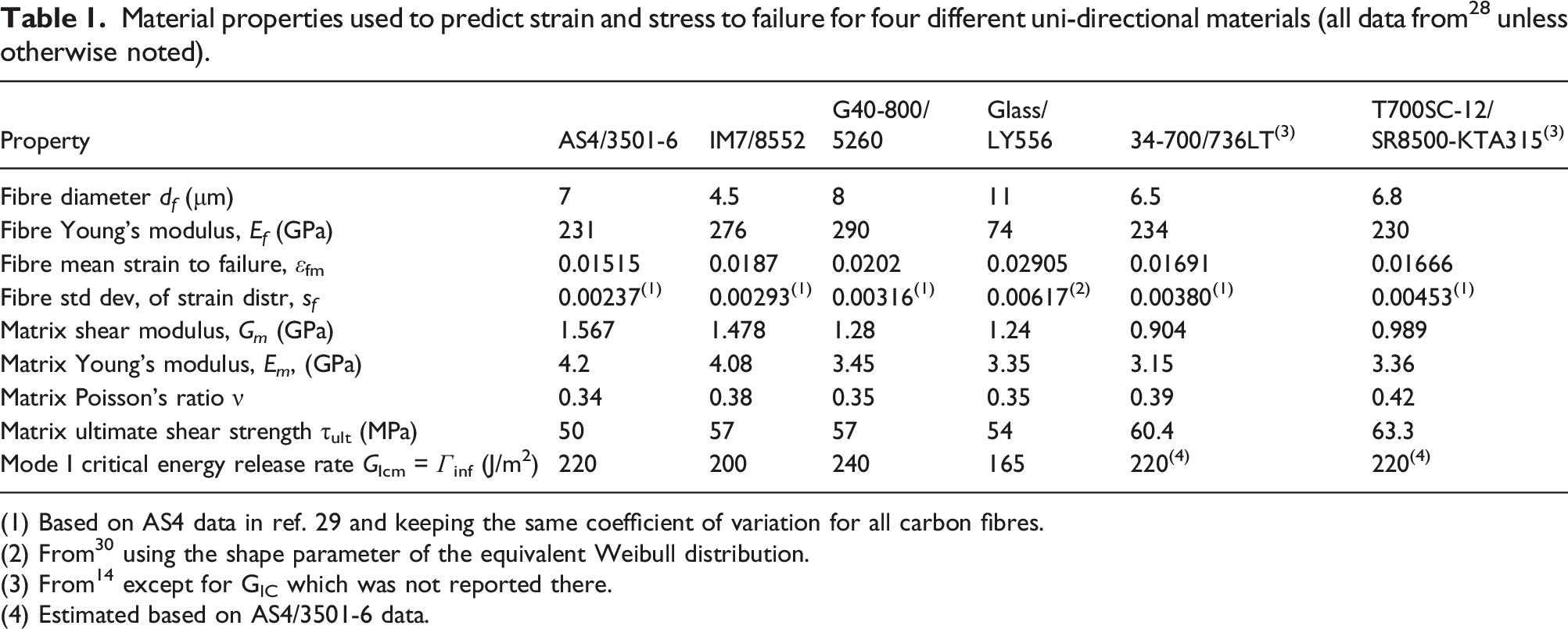
(1) Based on AS4 data in ref. 29 and keeping the same coefficient of variation for all carbon fibres.

(2) From³⁰ using the shape parameter of the equivalent Weibull distribution.

(3) From¹⁴ except for G_IC which was not reported there.

(4) Estimated based on AS4/3501-6 data.

Figure 3.

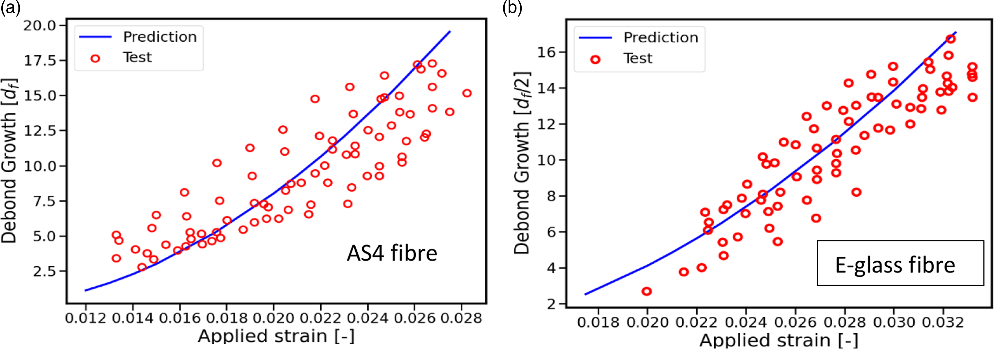
Interface crack length for AS4 (a) and E-glass (b) fragmentation tests compared to tests in ref. 27.

Inter-fibre radial matrix crack

If the fibre/matrix interface bond is stronger than the tensile strength of the matrix, a radial crack will form when the shear strength of the matrix is exceeded. Which of the two types of cracks is preferred is determined in the next section using an energy approach. For now the focus is a radial crack which will start at the tip of the fibre crack and will have length L_r as shown in the third image of Figure 1. The length L_r is estimated as the distance over which the energy from the shear stress exceeding the shear strength (shaded area in Figure 2) can be distributed using the critical energy release rate corresponding to the radial crack growth. As the critical energy release rate, G_Icm, the mode 1 critical energy release rate for the matrix is used. Then, analogous to equation (10):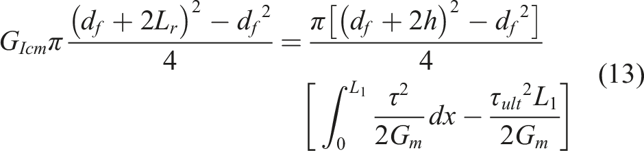

G_{I c m} π \frac{{(d_{f} + 2 L_{r})}^{2} - {d_{f}}^{2}}{4} = \frac{π [{(d_{f} + 2 h)}^{2} - {d_{f}}^{2}]}{4} [\int_{0}^{L_{1}} \frac{τ^{2}}{2 G_{m}} d x - \frac{{τ_{u l t}}^{2} L_{1}}{2 G_{m}}]

(13)

With L₁ given by equation (8). Solving for L_r gives:

L_{r} = \frac{d_{f}}{2} [\sqrt{1 + \frac{2 h (d_{f} + h)}{G_{m} G_{I c m}} [\frac{α}{32} {(\frac{2 u_{o}}{d_{e f f}})}^{2} \frac{{E_{f}}^{2}}{{(1 + e^{α d_{e f f}})}^{2}} (e^{2 α L_{1}} - e^{2 α d} e^{- 2 α L_{1}} - 4 α L_{1} e^{α d} - 1 + e^{2 α d}) - \frac{{τ_{u l t}}^{2} L_{1}}{{d_{f}}^{2}}]} - 1]

(14)

Fibre/matrix cracks versus inter-fibre radial matrix cracks

Equations (11) and (14) give the estimated crack sizes for the two extreme cases of creating an interface crack or a radial crack. Situations where a crack might start in one direction and branch out at some angle, see for example the work by Huang and Talreja³¹ which numerically modelled the problem for short fibre composites, are not discussed here. Within the context of the present discussion, intermediate cases are possible, where both types of cracks are present, with fibre/matrix interface cracks in one region of the ply and inter-fibre radial cracks in another see for example,³² Here, conditions under which one type of crack would be preferred over the other are discussed.

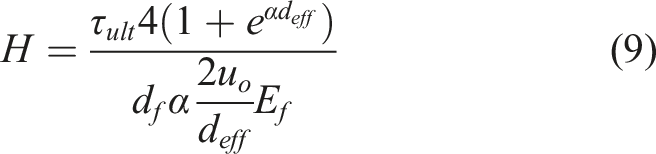
If a crack forms at the fibre/matrix interface, the portion of the fibre between the crack in the fibre and the tip of the interface crack is not loaded. The load in the fibre shears into the matrix. This situation is shown in Figure 4. There is a length L of the matrix which transfers the load, from shear load at the crack tip defined by the circumference AB, to axial tensile load at the tip of the crack interface along CD. This means that the normal stress in the fibre is zero from the fibre crack to the section AB. Effectively, the shear lag problem solved in the “Stress field around fibre crack” section has been moved to a new origin at section AB. Starting at that location, the solutions from the “Stress field around fibre crack” section for the normal stress in the fibre and the shear stress in the matrix are still valid. Thus, the superposition of two problems is shown in Figure 4: a cracked fibre at AB, with corresponding deflection u_o, and matrix under tension along the interface crack between AB and CD, with corresponding deflection u₁. The total deflection u_tot is the sum of u₀ and u₁.

Figure 4.

Region of unloading in the vicinity of a fibre/matrix interface crack.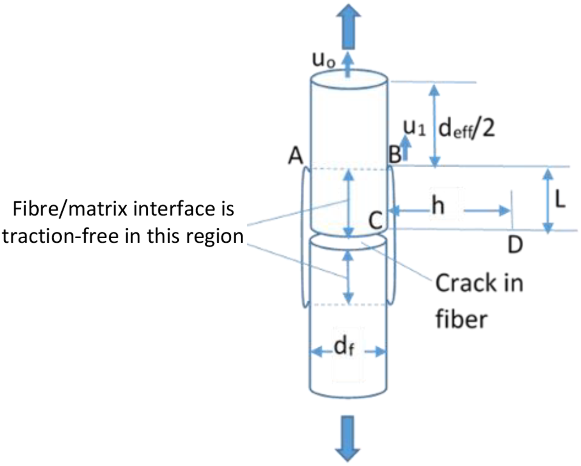

The situation, however, differs from that in the “Stress field around fibre crack” section in that the matrix portion between the crack in the fibre and the section AB undergoes combined loading. Thus, a given applied displacement to the composite consists of two contributions, a u_o displacement in the fibre at distance d_eff/2 from AB, and a matrix displacement u₁ at circumference AB. It is assumed that the displacement of the matrix at CD is zero by symmetry.

A representative volume element (RVE) is considered consisting of a portion of the cracked fibre of length d_eff/2 + L with L the length of the interface crack given by equation (11) and matrix surrounding it extending radially to the length h of equation (5) also shown in Figure 4. The energy stored in this RVE after an interface crack of length L is created can be calculated by computing the work done when ply stress σ_ply is applied. The total force acting on the RVE is obtained by multiplying the ply stress by the cross-sectional area of the RVE: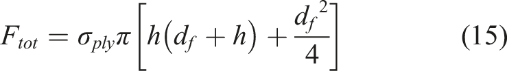

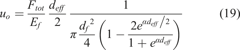
F_{t o t} = σ_{p l y} π [h (d_{f} + h) + \frac{{d_{f}}^{2}}{4}]

(15)

The total displacement of the RVE at L + d_eff/2 is given by:

u_{t o t} = u_{o} + u_{1}

(16)

Treating the situation as a one-dimensional problem, the strain u_o/(d_eff/2) can be related to the applied stress and, from that, the displacement u_o can be obtained: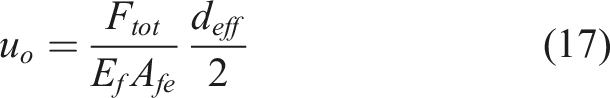

u_{o} = \frac{F_{t o t}}{E_{f} A_{f e}} \frac{d_{e f f}}{2}

(17)

Note that the area A_fe accounts for the fact that the stress in the fibre is evaluated at d_eff/2 where, as shown in the “Stress field around fibre crack” section, 99% of the (uncracked) fibre stress is recovered. Thus, evaluating equation (2) at x=d_eff/2: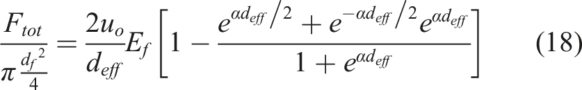

\frac{F_{t o t}}{π \frac{{d_{f}}^{2}}{4}} = \frac{2 u_{o}}{d_{e f f}} E_{f} [1 - \frac{e^{α d_{e f f} / 2} + e^{- α d_{e f f} / 2} e^{α d_{e f f}}}{1 + e^{α d_{e f f}}}]

(18)

which, after some rearranging, leads to:

u_{o} = \frac{F_{t o t}}{E_{f}} \frac{d_{e f f}}{2} \frac{1}{π \frac{{d_{f}}^{2}}{4} (1 - \frac{2 e^{α d_{e f f} / 2}}{1 + e^{α d_{e f f}}})}

(19)

Comparing with equation (17):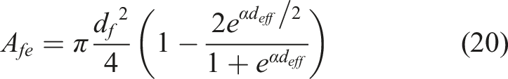

A_{f e} = π \frac{{d_{f}}^{2}}{4} (1 - \frac{2 e^{α d_{e f f} / 2}}{1 + e^{α d_{e f f}}})

(20)

Now the matrix displacement u₁ is given by: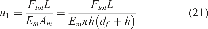

u_{1} = \frac{F_{t o t} L}{E_{m} A_{m}} = \frac{F_{t o t} L}{E_{m} π h (d_{f} + h)}

(21)

With L the interfacial crack length given by equation (11) and E_m is the matrix Young’s modulus. Combining: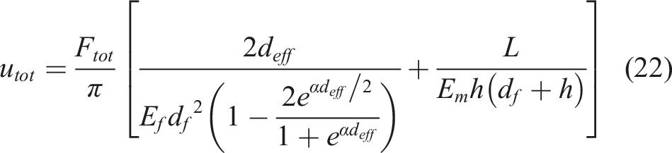

u_{t o t} = \frac{F_{t o t}}{π} [\frac{2 d_{e f f}}{E_{f} {d_{f}}^{2} (1 - \frac{2 e^{α d_{e f f} / 2}}{1 + e^{α d_{e f f}}})} + \frac{L}{E_{m} h (d_{f} + h)}]

(22)

Therefore, the energy stored in the RVE when σ_ply is applied right after an interface crack of length L is created, is equal to the work done by the applied force:

U_{R V E} = \frac{F_{t o t} u_{t o t}}{2}

(23)

For an inter-fibre crack, the situation is analogous with F_tot the same as in equation (15) but u_tot now given by:

u_{t o t} = u_{o} + δ

(24)

Here δ is the crack mouth opening displacement for the radial matrix crack emanating from the fibre crack. This is shown in Figure 5 where it is assumed that the fibres surrounding the cracked fibre do not have cracks lining up with the radial crack shown in the Figure. For the case of an axially loaded cylinder with a crack, the displacement δ was calculated by Nied and Erdogan.²³ The present case is not exactly the same because the load from the fibre is applied to the matrix through shear and causes a small local bending moment. However, the Nied-Erdogan result will be used as an approximation. The tabulated values reported in ref. 23 are interpolated here in determining δ.

Figure 5.

Inter-fibre crack emanating from cracked fibre in a uni-directional composite.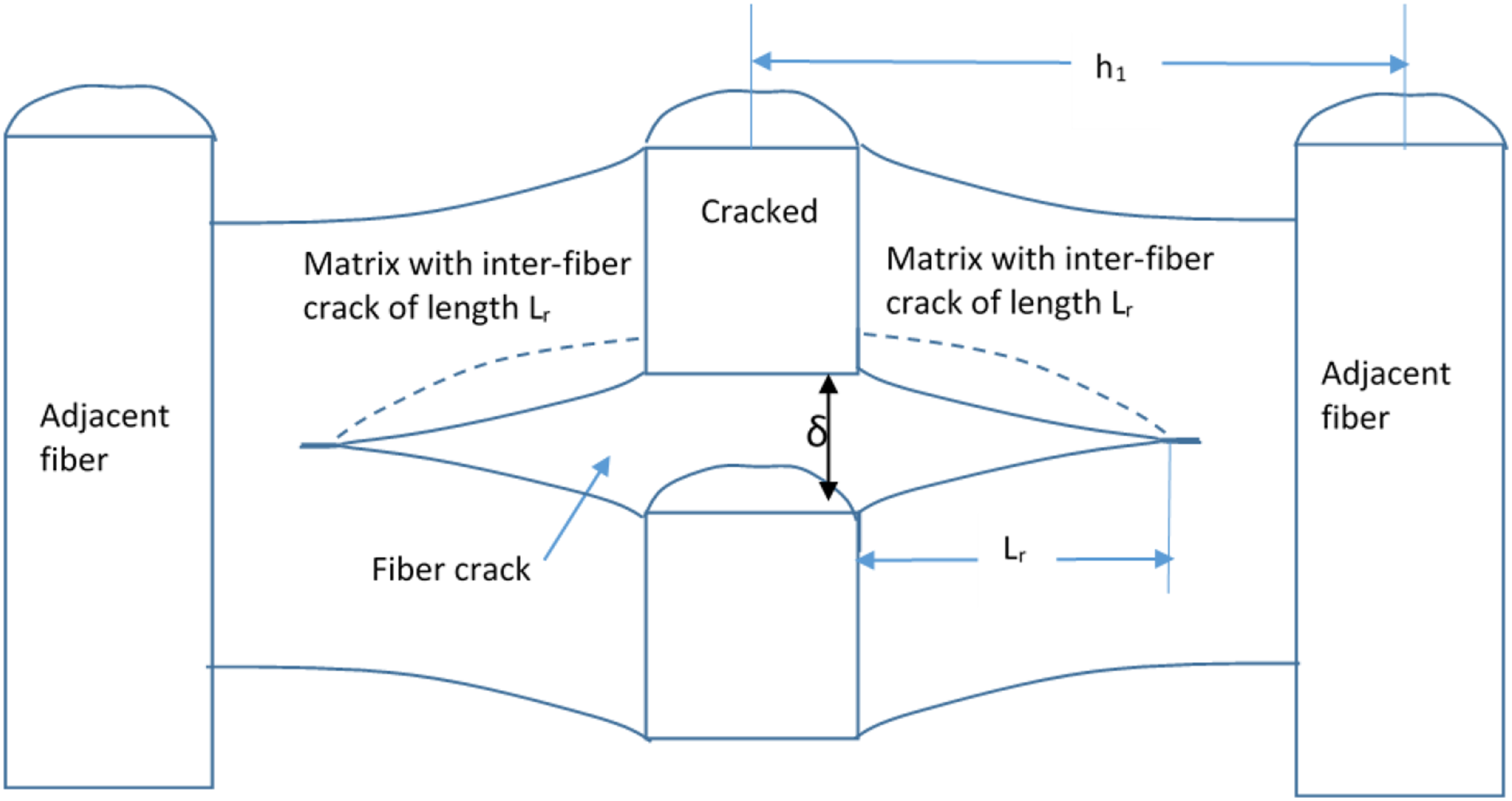

For a given value of σ_ply, the displacement u_o changes when a crack appears. It can be computed by accounting for the fact that some fibres in the ply are cracked and some are not. Denoting by f the fraction of cracked fibres: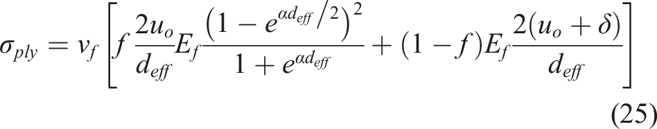

σ_{p l y} = v_{f} [f \frac{2 u_{o}}{d_{e f f}} E_{f} \frac{{(1 - e^{α d_{e f f} / 2})}^{2}}{1 + e^{α d_{e f f}}} + (1 - f) E_{f} \frac{2 (u_{o} + δ)}{d_{e f f}}]

(25)

In this relation, the first term in brackets is the stress in the cracked fibres obtained using equation (2) and the second term is the stress in the intact fibres obtained by multiplying the Young’s modulus by the strain u_tot/(d_eff/2). The fibre volume fraction v_f in front of the brackets is used to go from fibre stresses to ply stresses. Solving equation (25) for u_o:

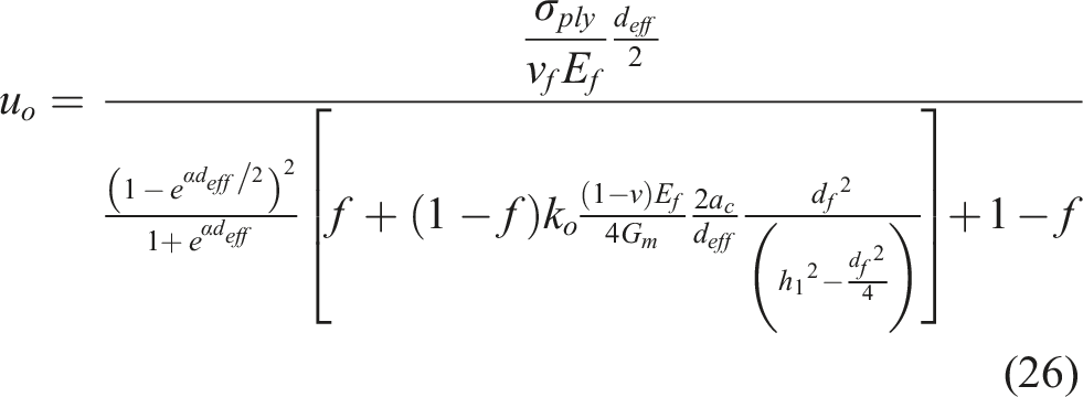
u_{o} = \frac{\frac{σ_{p l y}}{v_{f} E_{f}} \frac{d_{e f f}}{2}}{\frac{{(1 - e^{α d_{e f f} / 2})}^{2}}{1 + e^{α d_{e f f}}} [f + (1 - f) k_{o} \frac{(1 - ν) E_{f}}{4 G_{m}} \frac{2 a_{c}}{d_{e f f}} \frac{{d_{f}}^{2}}{({h_{1}}^{2} - \frac{{d_{f}}^{2}}{4})}] + 1 - f}

(26)

The fraction of cracked fibres f in equation (26) is found by assuming that the strain-to-failure of dry fibres is normally distributed with known mean and standard deviation (see next section). This fraction f can be applied to any region of the material which contains a sufficiently large number of fibres which represent the statistical distribution of fibre strain to failure. In equation (26), a_c = L_r is the crack length and k_o is a constant of proportionality in the Nied-Erdogan relation:²³

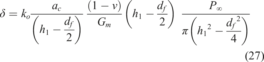
δ = k_{o} \frac{a_{c}}{(h_{1} - \frac{d_{f}}{2})} \frac{(1 - ν)}{G_{m}} (h_{1} - \frac{d_{f}}{2}) \frac{P_{\infty}}{π ({h_{1}}^{2} - \frac{{d_{f}}^{2}}{4})}

(27)

The length h₁ is the radius of the “cylinder” of interest which, here, is taken to be the center-to-center distance between adjacent fibres. P_∞ in equation (27) is the load applied on the fibre and is given by:

P_{\infty} = σ_{f} π \frac{{d_{f}}^{2}}{4}

(28)

Then, placing equations (15) and (26) in equation (23) gives the energy U_RVE stored in an RVE with a radial inter-fibre crack.

A comparison of U_RVE values for interface and inter-fibre cracks is in order. This is done by applying the above equations to the cases of the AS4/3501-6 carbon/epoxy and E-glass/epoxy materials for varying fibre volume fraction. For these materials, properties were obtained from Kaddour et al.²⁸ shown in Table 1 and from Kim and Nairn.²⁷ The ratio of the RVE energy for interface crack divided by that for an inter-fibre crack is shown in Figure 6 as a function of fibre volume fraction v_f.

Figure 6.

Comparison of energy stored in RVE for interface and inter-fibre cracks for two materials.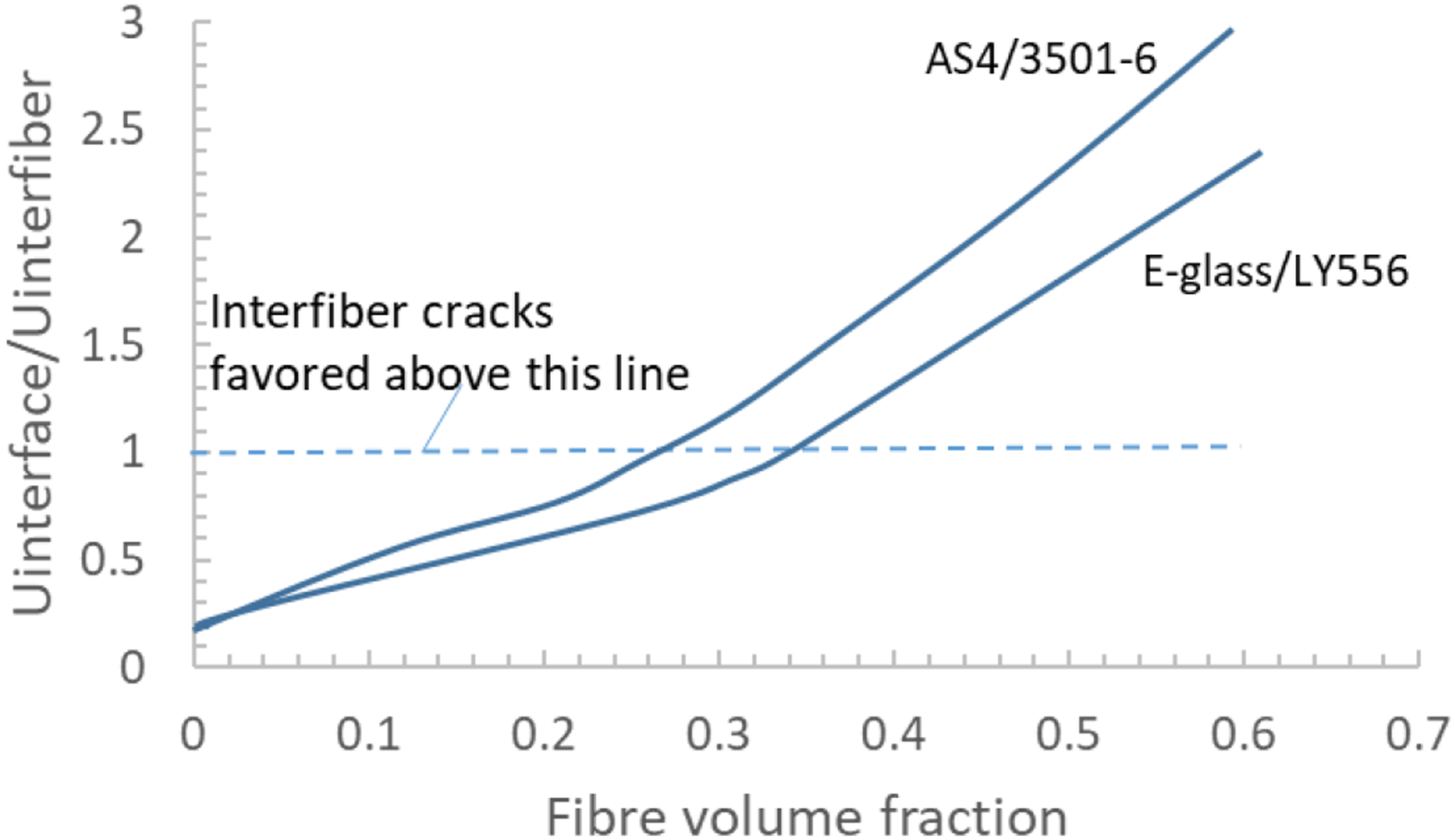

According to Figure 6, for fibre volume fractions higher than, approximately, 0.26 the carbon/epoxy, and 0.34 for the glass epoxy material, the energy in a RVE with interface crack is higher so it is not the preferred configuration. Therefore, in this case, for fibre volumes higher than these values, inter-fibre cracks will be the mode of energy dissipation. For lower fibre volumes, interface cracks will be preferred. Obviously, as shown by the differences between the two materials used in Figure 6, the changeover value will be different for different fibre-matrix combinations.

It is important to keep in mind that, in an actual ply, the fibre array is not regular. There are regions where fibres are close together, exceeding the average inter-fibre spacing, and regions where they are far apart where the local inter-fibre spacing may be significantly lower than the average. Thus, there will be situations where interface and inter-fibre cracks will both be present at different locations depending on how the fibres are distributed.

Stiffness of a 0° uni-directional ply after fibre cracking

The Young’s modulus of a 0° ply after fibres start to crack can now be determined. For low fibre volume fractions, where, as demonstrated in the previous section, interface cracks between fibre and matrix are favoured, the residual Young’s modulus 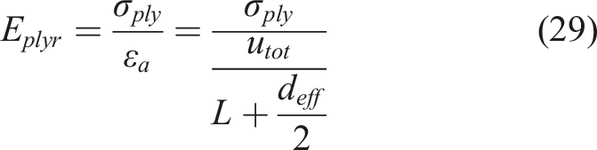$E_{p l y r}$ for a ply under stress σ_ply is given by:

E_{p l y r} = \frac{σ_{p l y}}{ε_{a}} = \frac{σ_{p l y}}{\frac{u_{t o t}}{L + \frac{d_{e f f}}{2}}}

(29)

With u_tot given by equation (16) and L given by equation (11). For high fibre volume fractions, where inter-fibre radial matrix cracks are favoured, using u_tot from equation (24), the Young’s modulus is shown to be: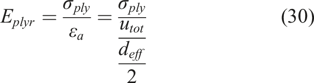

E_{p l y r} = \frac{σ_{p l y}}{ε_{a}} = \frac{σ_{p l y}}{\frac{u_{t o t}}{\frac{d_{e f f}}{2}}}

(30)

Strength of a 0° uni-directional ply

The details of load redistribution in the vicinity of a broken fibre and subsequent load increase have been addressed by Zhuang et al.³³ However, that work did not give detailed comparisons of predictions of ply strength to test results. In another multi-scale numerical approach, Qian et al.³⁴ have started from single failed fibres and numerically scaled predictions through different unit cells to simulate static and fatigue failure of uni-directional plies. In that work, the positions of the fibres surrounding the broken fibre were chosen randomly to better represent actual fibre distributions in a ply. It should be noted that, in all these cases, the stress concentration factor on fibres next to a broken fibre was low, never exceeding 1.13.

Here, the analytical approach presented in previous sections is used to predict tensile failure of a 0° uni-directional ply and compare with test results. This is done using, exclusively, properties of the individual constituents, the fibre and matrix. For the relatively high fibre volume fractions of interest here, greater than 0.45, it is assumed that the fibres are arranged in a hexagonal array as shown in Figure 7. Under tensile load, perpendicular to the page in Figure 7, some fibres will crack.

Figure 7.

Hexagonal fibre array for uni-directional material.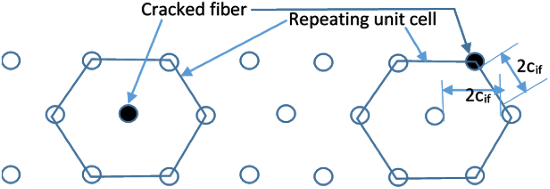

The strain to failure of dry fibres is normally distributed with mean ε_fm and standard deviation s_f. Since, in a typical ply, there are billions of fibres, it is reasonable to assume that fibres of all strains to failure, covering the complete statistical distribution, are present in the array. Then, the fraction of cracked fibres f when strain ε_a is applied can be determined as the probability that the strain of any given fibre be lower than ε_a:

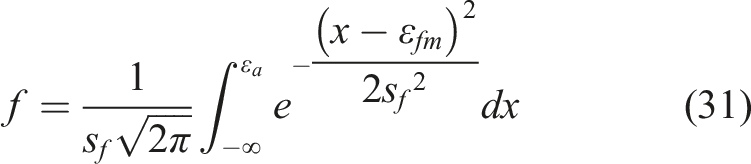
f = \frac{1}{s_{f} \sqrt{2 π}} \int_{- \infty}^{ε_{a}} e^{- \frac{{(x - ε_{f m})}^{2}}{2 {s_{f}}^{2}}} d x

(31)

It should be noted that, for typical materials (see Table 1) with typical ply thicknesses, equation (31) predicts that at least 0.004 strain must be applied before one fibre per unit of ply width cracks for carbon/epoxy materials while one fibre per unit of ply width will be cracked during manufacturing (zero applied strain) for the glass/epoxy. Having a small number of cracked fibres in the as manufactured state is not uncommon. Therefore, the approximation in equation (31) of using minus infinity as the lower limit and allowing zero strains to crack fibres has negligible effect on the fraction f predicted by equation (31). It is recognized here that the fibre failure strain is a function of gauge length. In this work, the mean and standard deviation values typical of longer fibres (longer than 5–10 cm) are used since they represent the fibre lengths used in the test specimens with which the predictions will be compared.

As the strain applied to the ply increases, the size of the inter-fibre radial crack created increases and is given by equation (14). For low applied strains, f is small and the cracked fibres are very sparsely distributed within the ply. For higher strains, f increases and a situation is reached where, on an average sense, one fibre in every repeating unit cell is cracked. Two such cracked fibres, representing the two extremes, are shown as filled circles in Figure 7. There are two possibilities; either the cracked fibre will be at the center of the unit cell as shown on the left of Figure 7, or on the boundary as shown on the right of the Figure. The unit cell consists of one full fibre and one third portions of six surrounding fibres forming a regular hexagon, for a total fibre area corresponding to the area of three fibres. So for the first case, where the fibre at the center has cracked, 1/3 or 33% of the fibres are cracked on an average sense. For the second case, where the cracked fibre is on the boundary, one third of that fibre belongs to the unit cell so 1/9 or 11% of the fibres are cracked. These percentages, even though they represent average behaviour and not the typical random behaviour of a ply are important in predicting ply failure.

A strain ε_a, corresponding to a given ply stress is applied to the ply. A fraction f of the fibres given by equation (31) develops cracks. If that strain is such that the maximum shear stress in equation (4) exceeds the shear strength of the matrix, then interface or inter-fibre cracks develop as discussed in the “Fibre/matrix cracks versus inter-fibre radial matrix cracks” section. For typical materials with high fibre volume fractions, inter-fibre cracks will develop as was shown in Figure 6. The length of these cracks L_r is determined from equation (14). Let the average distance between the edge of one fibre and that of the next be 2 c_if, as seen in Figure 7. For hexagonal arrays, half that distance is: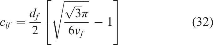

c_{i f} = \frac{d_{f}}{2} [\sqrt{\frac{\sqrt{3} π}{6 v_{f}}} - 1]

(32)

Then, the following cases are distinguished using the 11% (one cracked fibre per unit cell) and 22% (two cracked fibres per unit cell) determined above:

(a) ε_a is lower than the strain for which maximum shear stress in the matrix exceeds τ_ult in the matrix: f fibres have cracked but there is no ply failure.

(b) ε_a is such that the maximum shear stress in the matrix exceeds τ_ult. The fraction f and the inter-fibre crack length L_r are calculated.

1. If f < 0.11 and L_r < c_if there is no failure because the cracked fibres are very few and isolated and even if they are ineffective in carrying load when L_r ≥ c_if, there are still enough fibres effective.

2. If 0.11 ≤ f ≤ 0.22, the situation is as in Figure 7 where, on the average, at least one fibre in each unit cell is cracked. If L_r ≥ 2c_if the cracked fibre is ineffective in carrying load and, with the matrix crack extending to the adjacent fibres, the adjacent fibres are also (partially) ineffective. The ply fails. If L_r < c_if there is no failure and the applied strain can be increased.

3. If f ≥ 0.22, on the average, at least two fibres per unit cell have cracked. Then, if L_r ≥ c_if the matrix crack extends to, at least, the half-way point between adjacent fibres. With, on the average, two fibres cracked per unit cell, there is a high probability that the matrix crack emanating from one fibre will meet that emanating from the other again rendering them ineffective in carrying load. The ply fails. Note that in this case, the strain must be high enough such that there is a good chance that at least one crack in one cracked fibre (nearly) aligns with one crack in the other cracked fibre.

4. Once the strain causing failure ε_af has been reached, in cases (b2) or (b3) above, the corresponding ply stress is obtained from:

σ_{p l y f} = v_{f} E_{f} ε_{a f}

(33)

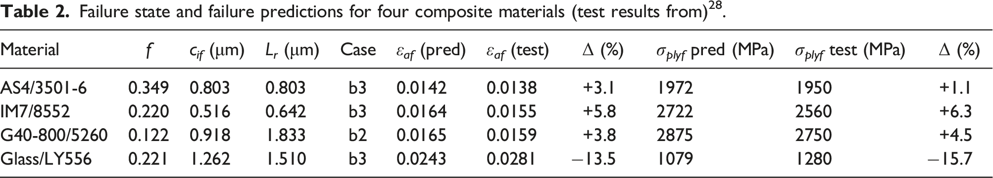
Note that equation (33) is only valid at failure where the inter-fibre crack forms and instantaneously grows across the ply. If there is no failure, equation (25) is valid. This procedure is summarized in Figure 8 and was applied to four different uni-directional materials, three carbon/epoxy and one glass/epoxy, and the strain and stress to failure were calculated. The fibre volume fraction in all cases was 0.6 so, according to Figure 6, inter-fibre cracks are favoured. The data needed for the calculations and the experimental results to compare to were taken from Kaddour et al.²⁸ Greenfield et al.²⁹ and Qian.³⁰ The relevant values and their source are given in columns 2–5 of Table 1.

Figure 8.

Flowchart for the approach for static and fatigue analysis.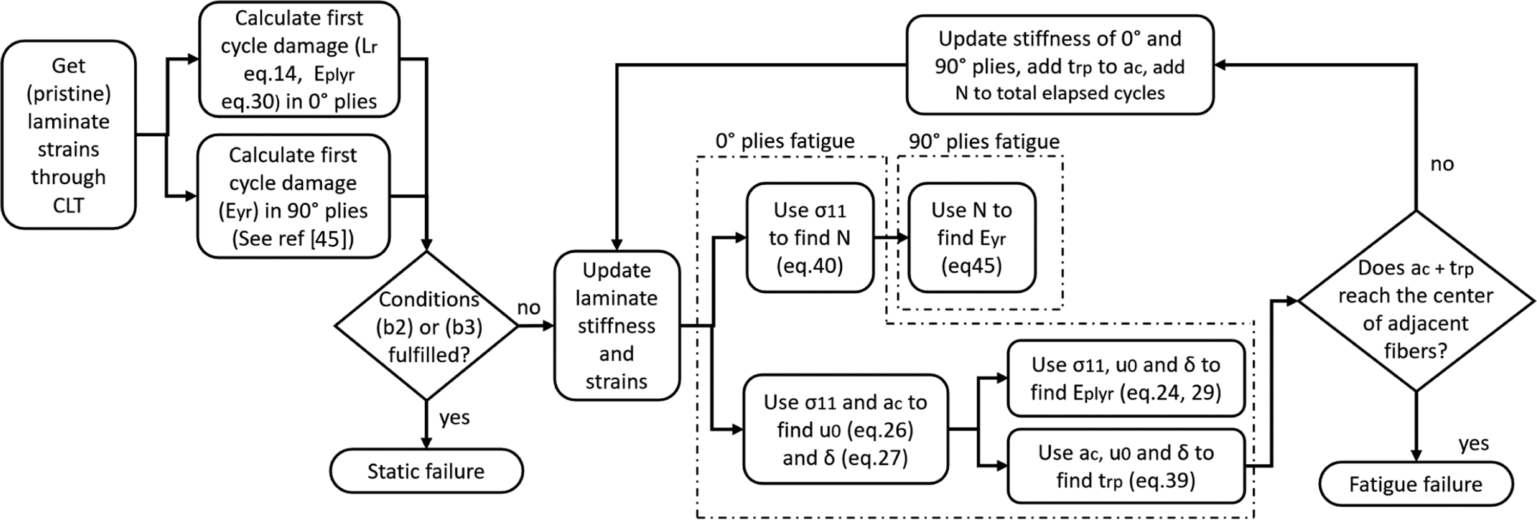

For each laminate, a strain was applied (=u_o/(d_eff/2)) and equation (31) was used to determine the fraction of cracked fibres f. Also, equation (14) was used to determine the inter-fibre radial crack length L_r. Then, the logic just described was applied to estimate the failure stress and strain of each material.

The predictions are compared to test results from²⁸ in Table 2. The fifth column in Table 2 shows the failure scenario, with (b2) and (b3) corresponding to the two possibilities described above: If the fraction f of cracked fibres, in column two, is less than 0.22, the inter-fibre crack length L_r, shown in the fourth column of the Table must be at least equal to the distance between adjacent fibres, 2c_if, with half that value shown in the third column. If f is greater than 0.22, the crack length must be at least equal to c_if, half the distance between fibres. It is seen that there is excellent agreement between predictions and test for failure strain and stress for the three carbon/epoxy materials (first three rows in Table 2) with biggest discrepancy 6.3%. For the case of glass/epoxy (fourth row in Table 2) the agreement is good with 15.7% difference between test and prediction. Inaccuracies in the mean and standard deviation of the fibre failure strain used in equation (31) could be a reason for the bigger discrepancy for glass/epoxy.

Table 2.

Failure state and failure predictions for four composite materials (test results from)²⁸.

Material	f	c_if (μm)	L_r (μm)	Case	ε_af (pred)	ε_af (test)	Δ (%)	σ_plyf pred (MPa)	σ_plyf test (MPa)	Δ (%)
AS4/3501-6	0.349	0.803	0.803	b3	0.0142	0.0138	+3.1	1972	1950	+1.1
IM7/8552	0.220	0.516	0.642	b3	0.0164	0.0155	+5.8	2722	2560	+6.3
G40-800/5260	0.122	0.918	1.833	b2	0.0165	0.0159	+3.8	2875	2750	+4.5
Glass/LY556	0.221	1.262	1.510	b3	0.0243	0.0281	−13.5	1079	1280	−15.7

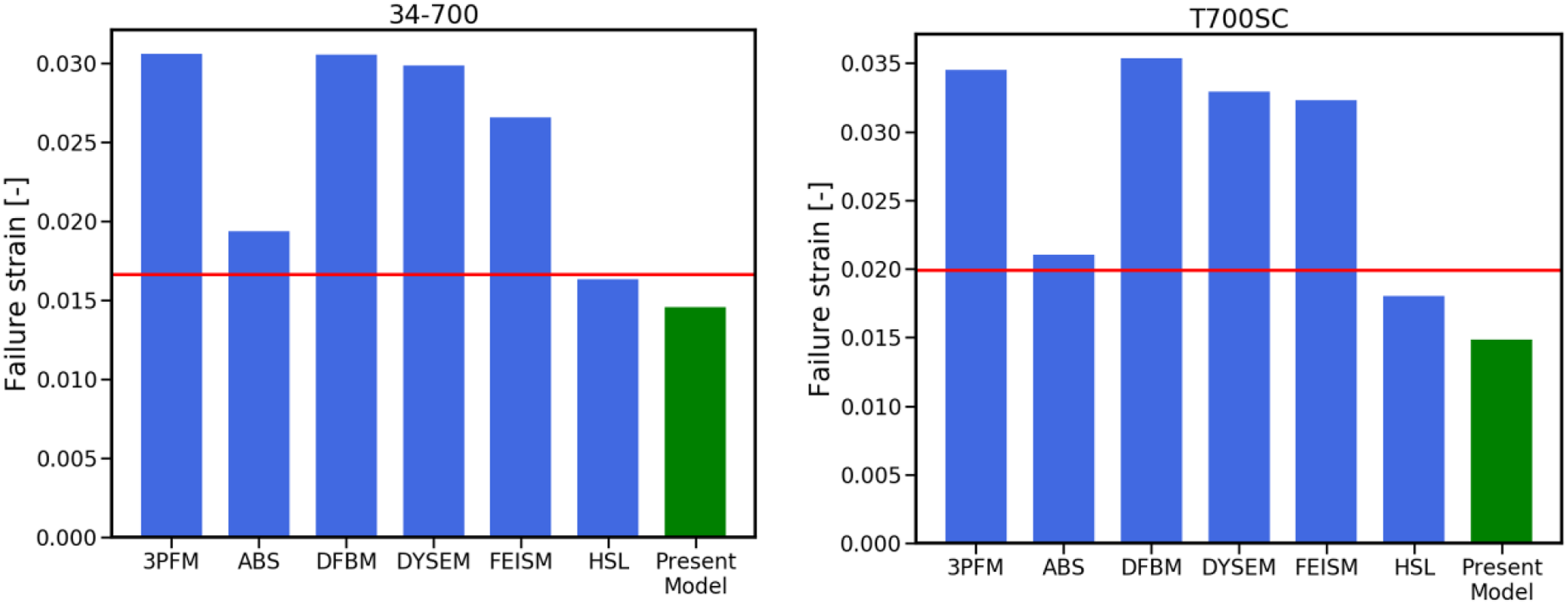
A further comparison was done with the test results and predictions from six models in ref. 14 These are a 3D progressive failure model (3PFM), an analytically based strength simulation (ABS), a dispersed fibre breaks model (DFBM), a dynamic spring element model (DYSEM), a finite element imposed stress model (FEISM) and a hierarchical scaling law model (HSL). The results for ultimate strains for two different materials are shown in Figure 9. For both materials, the present model is in good agreement with test and the third best among the seven models shown in Figure 9 in terms of accuracy.

Figure 9.

Ultimate strain predictions from present model (green bar) compared to test results (horizontal line) and six other models from.¹⁴

Extension to fatigue

Fatigue of 0° ply

Load control is assumed. With minor modifications the approach can also be applied to stroke control cases. During the first cycle, with no matrix cracks, the strain corresponding to the constant stress σ_ply is given by: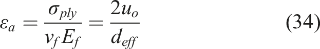

ε_{a} = \frac{σ_{p l y}}{v_{f} E_{f}} = \frac{2 u_{o}}{d_{e f f}}

(34)

Under this stress, if the shear strength of the matrix is locally exceeded, a radial inter-fibre crack will be created of length L_r given by equation (14). As the second cycle is applied, a plastic zone of dimension t_rp forms ahead of the crack tip as shown in Figure 10. Using plain strain conditions, the size of the plastic zone is given by:

t_{r p} = {(1 - 2 ν)}^{2} \frac{{K_{1}}^{2}}{π {σ_{y}}^{2}}

(35)

Figure 10.

Matrix plastic zone forming ahead of an inter-fibre crack.

With ν, σ_y the Poisson’s ratio and yield stress of the matrix and K₁ the stress intensity factor. K₁ is obtained by doing a best fit of the constant k shown in equation (36) below, which is tabulated in ref. 23

K_{1} = k \frac{P_{\infty} \sqrt{a_{c}}}{π (b^{2} - a^{2})} = k \frac{P_{\infty} \sqrt{a_{c}}}{π ({h_{1}}^{2} - \frac{{d_{f}}^{2}}{4})}

(36)

In equation (36), a_c is the running crack size with starting value L_r. P_∞ is the far field axial load given by equation (28), a is the fibre radius and b is half of h₁ the radius of matrix material analysed around the fibre shown in Figure 5. Note that here the term “crack size” refers to the radial length of the crack from the fibre surface to the crack front. The total fibre displacement at d_eff/2 is given by equation (24) with u_o and δ given by equations (26) and (27). The fibre stress needed in equation (28) is given by equation (2) evaluated at d_eff/2:

σ_{f} = \frac{2 u_{o}}{d_{e f f}} E_{f} \frac{{(1 - e^{α d_{e f f} / 2})}^{2}}{1 + e^{α d_{e f f}}}

(37)

Note that, here, 2u_o/d_eff is used instead of ε_a from equation (34) because, during fatigue cycling with constant maximum stress, the two are no longer equal. Combining with equation (24), ε_a during fatigue cycling is given by: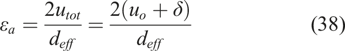

ε_{a} = \frac{2 u_{t o t}}{d_{e f f}} = \frac{2 (u_{o} + δ)}{d_{e f f}}

(38)

Thus, if u_o and δ are known, the size of the plastic zone t_rp can be determined. It can be seen from equations (27) and (28) that δ is a function of u_o through equation (37). Therefore, to determine t_rp, it suffices to determine u_o. This is done by requiring that the ply stress remains constant and equal to σ_ply. The ply stress will be a combination of the stress in the cracked fibres and the stress in the un-cracked fibres multiplied by the fibre volume fraction. The stress in cracked fibres is given by σ_f from equation (37) and the stress in un-cracked fibres is given by E_fε_a with ε_a given by equation (38). Combining and using f for the cracked fibre ratio and (1-f) for the un-cracked, gives σ_ply and u_o as obtained in equations (25) and (26). Substituting back in equation (35) gives the size of the plastic zone: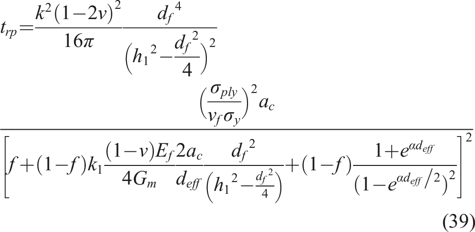

t_{r p} = \frac{k^{2} {(1 - 2 ν)}^{2}}{16 π} \frac{{d_{f}}^{4}}{{({h_{1}}^{2} - \frac{{d_{f}}^{2}}{4})}^{2}} \frac{{(\frac{σ_{p l y}}{v_{f} σ_{y}})}^{2} a_{c}}{{[f + (1 - f) k_{1} \frac{(1 - ν) E_{f}}{4 G_{m}} \frac{2 a_{c}}{d_{e f f}} \frac{{d_{f}}^{2}}{({h_{1}}^{2} - \frac{{d_{f}}^{2}}{4})} + (1 - f) \frac{1 + e^{α d_{e f f}}}{{(1 - e^{α d_{e f f} / 2})}^{2}}]}^{2}}

(39)

Now the stress in the plastic zone is equal to the yield stress of the matrix if we model it as elastic-perfectly plastic. Beyond the plastic zone the stress is lower than the yield stress and drops relatively quickly with distance. During subsequent cycles, there is no damage mechanism at the length scales discussed so far. At shorter scales, voids will be created and will coalesce inside the plastic zone but there is no mechanism presented here that can describe that process. Such mechanisms may be represented by a macroscopic model which covers them and relates the macroscopic applied stress σ_ply and the static failure strength of the ply to the cycles to failure:³⁵

N = {(\frac{σ_{f a i l}}{σ_{p l y}})}^{α_{w}}

(40)

where α_w, is the shape parameter of the two parameter Weibull distribution describing the strength of the ply corrected for stress ratio R,³⁵ and σ_fail is the static failure strength of the ply. Equation (40) is meant to capture shorter scale phenomena occurring in the region of highest stress in the matrix. So N represents the number of cycles to crack the plastic zone and extend the crack over a length equal to the plastic zone size.

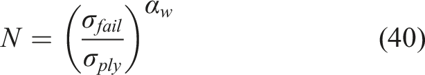
Therefore, starting with the second cycle, and provided the applied shear stress in the matrix exceeds the matrix yield strength, N cycles will take place and the plastic zone size will extend by the amount of equation (39). Then, the new crack size is a_c + t_rp. With this new crack size, a new plastic zone size is computed and another N cycles can be expended. Every time, the crack is extended by t_rp and the process is repeated. It should be noted that t_rp is not constant because the crack size increases and that affects the crack mouth displacement δ, the stress intensity factor K₁ and the fibre displacement u_o. Failure is assumed to occur when the crack reaches the center of the adjacent fibre. It is assumed that the toughness of the fibre is higher than that of the matrix and the inter-fibre crack goes around the adjacent fibre. Retardation effects due to the proximity of the adjacent fibre are not accounted for.

This radial crack is not growing in one location only. There will be multiple locations throughout the ply, first indicated by the fraction f of equation (31) and then, as cycling progresses, additional locations will develop similar damage zones due to wear-out and load redistribution from cracked to uncracked fibres. From the point of view of the creation of multiple damage zones leading to final failure when they grow to a critical size, the present method is, to an extent, analogous to the model proposed by Sørensen et al.³⁶ where damage zones created by longitudinal cracks reach a critical size. The difference is that the present method predicts either longitudinal or radial cracks depending on the local fibre volume (see Figure 6).

The above approach was applied to a uni-directional ply of the AS4/3501-6 material. For that material, the coefficient of variation for tensile strength is reported in ref. 37 as 5.62%. This can be translated to a shape parameter of a Weibull distribution using, for example the approximate expression in ref. 38. This, in turn, is corrected to account for stress ratio R = 0.1 instead of R = 0 with the approximation given in ref. 35. This gives α_w = 24.7051.

A note about the effect of the 3501-6 matrix yield stress is in order. For this material, there is a disagreement on its value between refs. 28,39,40. This may have to do with different batches of material being tested at different times. In the results presented below, the value 165.8 MPa reported in ref. 39,40. was used. However, the sensitivity of the predictions to that value was checked by also using the value of 69 MPa in ref. 28. It was found that the predicted cycles to failure change by about half a decade, which is well within typical experimental scatter in composites fatigue. More importantly, when the results are normalized by the predicted life, there is no discernible effect on the stiffness degradation curves of Figure 14.

Fitting the tabulated data in Nied and Erdogan,²³ the following expressions are obtained for the coefficients in the displacement δ and stress intensity factor K₁:

k_{o} \frac{a_{c}}{h_{e}} = 2.7344 \frac{a_{c}}{h_{e}}

(41)

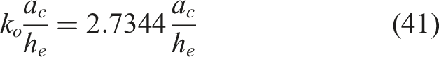
with “goodness of fit” R² = 0.9925

From which k_o in equation (27) equals 2.7344 and h_e = h₁-(d_f/2). Also,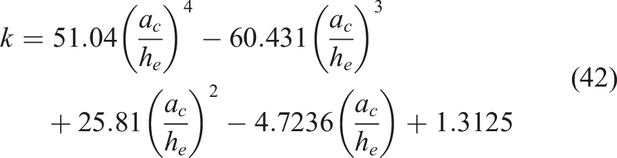

k = 51.04 {(\frac{a_{c}}{h_{e}})}^{4} - 60.431 {(\frac{a_{c}}{h_{e}})}^{3} + 25.81 {(\frac{a_{c}}{h_{e}})}^{2} - 4.7236 (\frac{a_{c}}{h_{e}}) + 1.3125

(42)

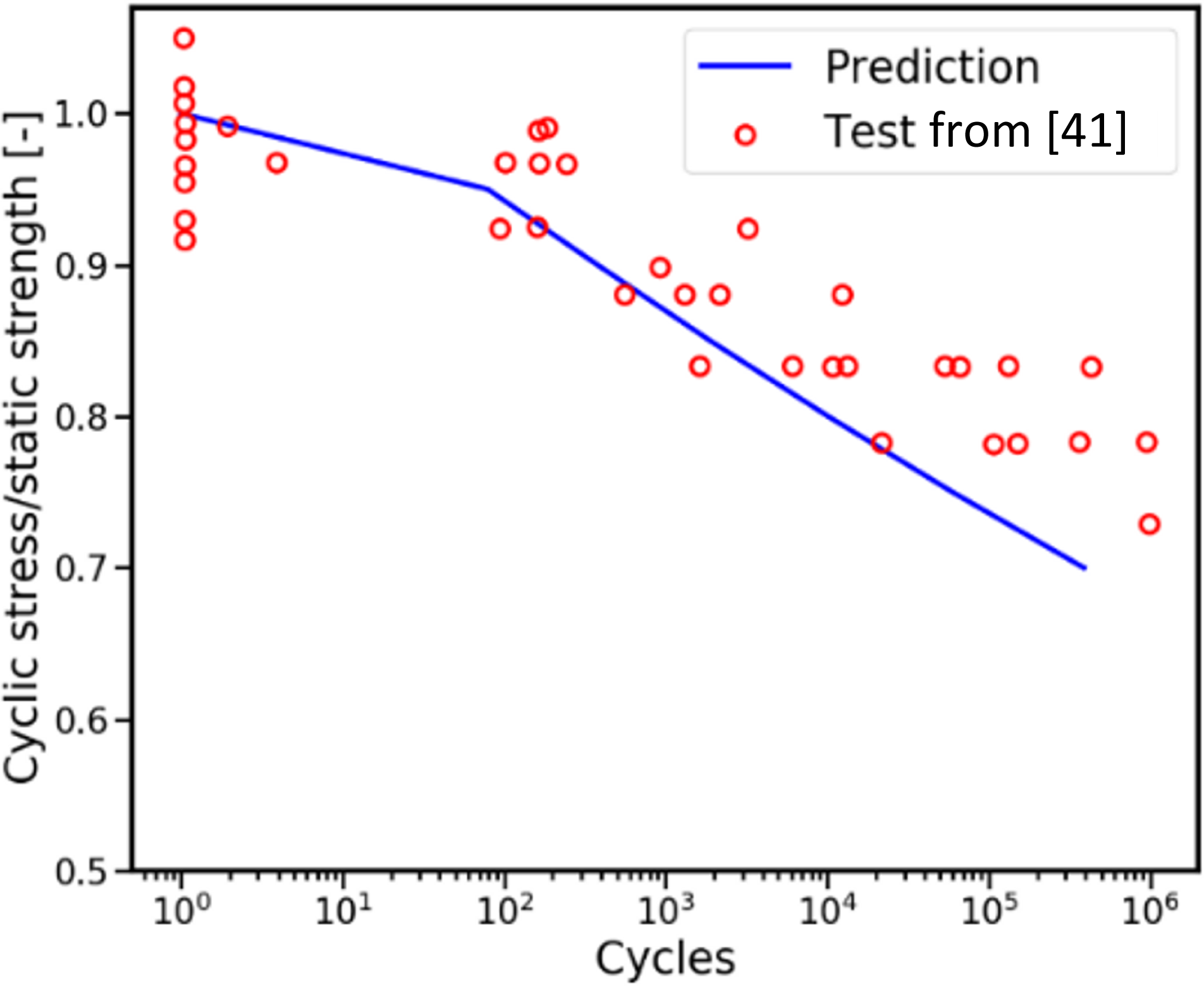
With R² = 0.9976 and k the constant in equation (36). Note that equations (41) and (42) are only valid for the parameter ratio a/b = 0.4 which is the case for AS4/3501-6 with fibre volume fraction equal to 0.6. Applying this approach and comparing to tests from Lee et al. in ref. 41 the results in Figure 11 are obtained. For each applied maximum cyclic stress, the cycles to failure are obtained by calculating the plastic zone size ahead of an inter-fibre crack using equation (39), determining the number of cycles to crack that plastic zone using equation (40), extending the crack and repeating the process until the crack has reached the nearest neighbour and the RVE can no longer carry load. Excellent agreement is observed. Only at high cycles, the predictions are on the conservative side.

Figure 11.

Fatigue curve for 0 ply of AS4-3501-6 material. Predictions compared to test results from.⁴¹

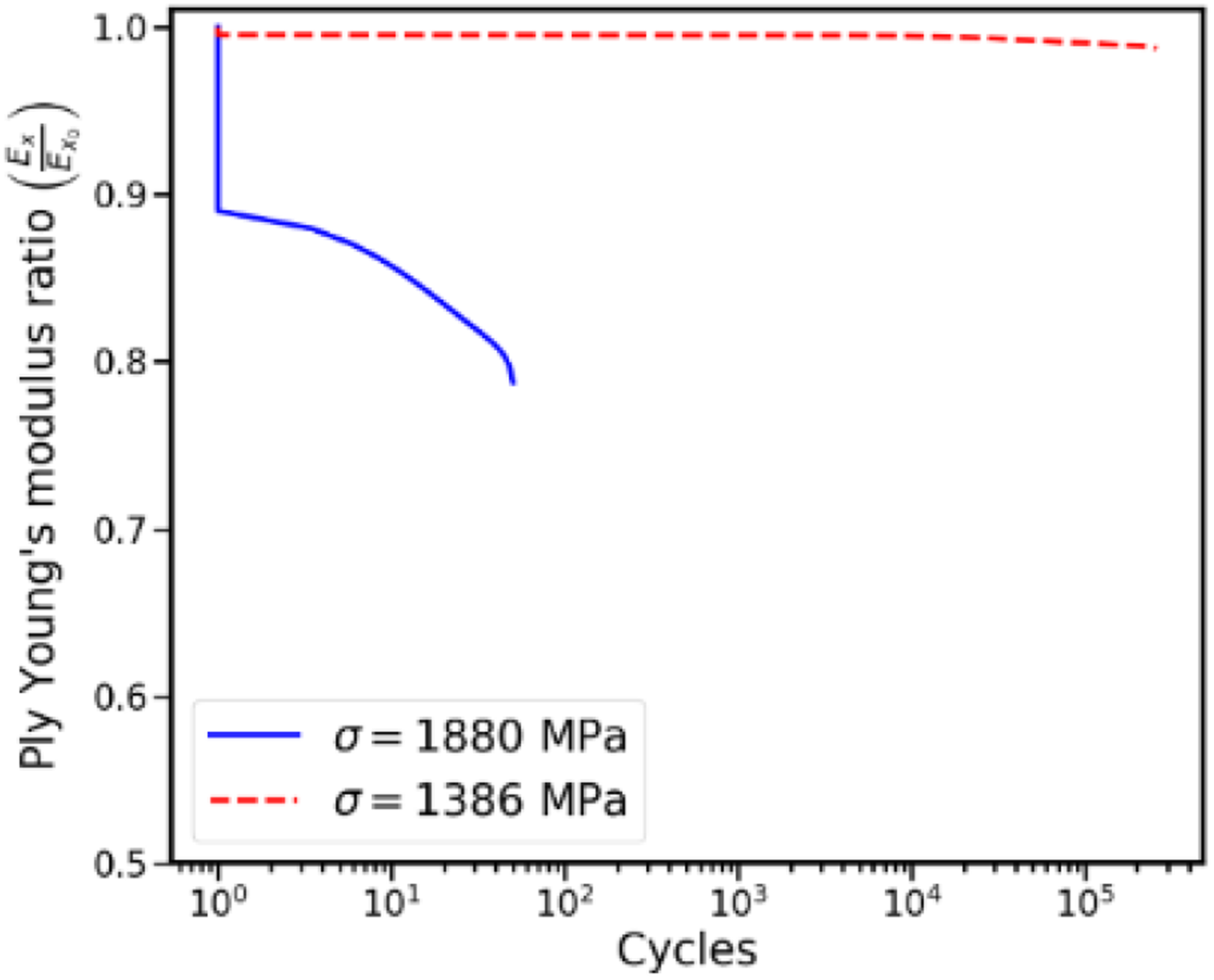
Also of interest are graphs of crack size and Young’s modulus as a function of cycles. These are shown in Figures 12 and 13 for R = 0.1 and applied stress of 1880 MPa. It is seen from Figure 12 that the crack increases almost linearly for most of the life and, near the end, growth becomes unstable. This “sudden death” behaviour is not uncommon. The ply Young’s modulus is shown in Figure 13 as a function of cycles for two different applied maximum stresses, 1880 (lower curve) and 1386 MPa (upper curve). It is interesting to note that, for higher applied stress, there is a sharp drop in stiffness at the beginning, which has been reported by many investigators [for example]^42–44 while for lower applied stress the reduction is less and more gradual. Near the end of life, the beginning of a sharp decrease in stiffness is observed for the lower curve, also reported by the same investigators. Such a decrease is not evident on the upper curve because failure at the end of life is sudden.

Figure 12.

Typical inter-fibre crack size versus cycles curve.

Figure 13.

Ply Young’s modulus ratio (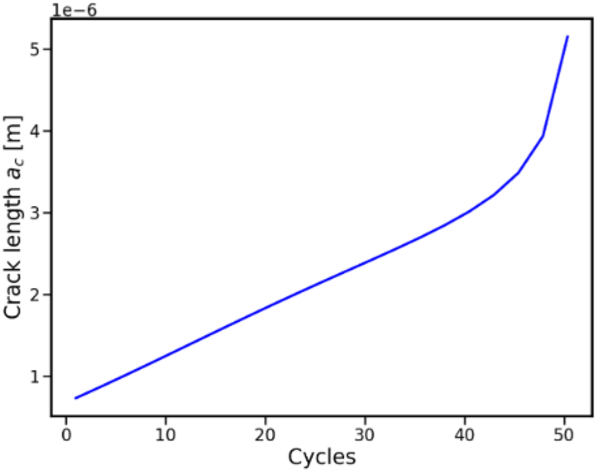 $E_{X} / E_{X 0})$ versus cycles for two load levels.

Fatigue of 90° ply

As illustrated in ref. 45 when loaded in transverse tension, plies will develop matrix cracks parallel to the fibres and perpendicular to the transverse direction. These cracks are randomly distributed at first, and as the strain increases and more cracks appear, their spacing becomes more uniform. Matrix cracks diminish the residual stiffness of the ply in the transverse direction, which can be expressed as: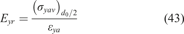

E_{y r} = \frac{{(σ_{y a v})}_{d_{0} / 2}}{ε_{y a}}

(43)

where

E_{y r}

is the residual

E_{2}

modulus of the ply,

ε_{y a}

is the applied transverse strain, and

{(σ_{y a v})}_{d_{0} / 2}

is the transverse tensile stress, averaged through the thickness at the midpoint between adjacent cracks.⁴⁵ The Poisson’s ratio ν₂₁ will also degrade at the same rate as E_yr, such that ν₂₁ = ν₁₂ E_yr/E₁₁. Following the model in ref. 45 matrix cracks will first appear when the transverse tensile stress in the ply matches the in situ transverse tensile strength

Y_{i s}^{t}

Consider a pristine ply, subject to a transverse tensile load low enough that $σ_{y} < Y_{i s}^{t}$ . A single application of such a load will only lead to the creation of few randomly distributed cracks, usually at the location of pre-existing defects (e.g. voids). If the same load is applied for a sufficient amount of cycles, the number of cracks will grow until they start forming regular, evenly distributed patterns. Further application of the same load over more cycles will increase the density of the evenly distributed matrix cracks.^43,46

As shown in ref. 45 for a single static load, a monotonic increase in crack density requires a monotonic increase in the applied load. If the load is constant, even after cracks have appeared in the first cycle, there is no damage mechanism at the length scales discussed here that could induce further cracking. It follows that the increase in crack density, seen in experiments^43,46 for a constant cyclic load must be governed by mechanisms at smaller scales. Such mechanisms can be represented by the macroscopic model from,³⁵ which this time relates the macroscopic transverse tensile stress 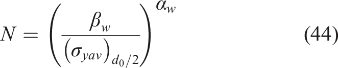${(σ_{y a v})}_{d_{0} / 2}$ and the static in situ transverse tensile strength $Y_{i s}^{t}$ of the ply to the cycles to failure:

N = {(\frac{β_{w}}{{(σ_{y a v})}_{d_{0} / 2}})}^{α_{w}}

(44)

where N represents the number of cycles to generate new matrix cracks. The variables α_w and β_w are, respectively, the shape and scale parameters of the two parameter Weibull distribution describing the in situ transverse tensile strength

Y_{i s}^{t}

of the ply, corrected for the stress-ratio R.³⁵ Equation (43) can also be used for a pristine ply, in which case

{(σ_{y a v})}_{d_{0} / 2}

would simply be replaced by

σ_{y}

. In essence, cyclic loading that does not immediately cause the appearance of new cracks within a single cycle, will cause the in situ transverse tensile strength

Y_{i s}^{t}

to degrade at a rate such that, after N cycles, it matches the transverse applied stress,³⁵ which is

σ_{y}

for a pristine ply or

{(σ_{y a v})}_{d_{0} / 2}

for a cracked ply. By solving equation (44) for

{(σ_{y a v})}_{d_{0} / 2}

and filling in the result in equation (43), the residual transverse modulus

E_{y r}

of a ply as a function of the applied cycles N is defined.

E_{y r} = \frac{β_{w}}{{ε_{y a} N}^{({1 / α}_{w})}} w i t h {(σ_{y a v})}_{d_{0} / 2} = \frac{β_{w}}{N^{({1 / α}_{w})}}

(45)

where

ε_{y a}

should take into account the most “current” damage state, due to either static or fatigue loading, meaning that the residual stiffness of the laminate should, for example, be updated after some of its plies develop cracks in the 1^st cycle. It is important to use a realistic and updated

ε_{y a}

since the intensity of the applied load and the extent of existing damage are implicitly included in its value.

Fatigue of cross-ply laminates

The methods shown in the “Fatigue of 0° ply” and “Fatigue of 90° ply” sections can be combined to predict the residual stiffness and failure of cross-ply laminates under cyclic uniaxial tension. First-cycle damage in the 0° plies can be predicted through the approach illustrated in the “Strength and stiffness of a 0° unidirectional tape ply”, while for the 90° plies the approach from⁴⁵ should be used. It is assumed that there is no damage interaction between the 0° and 90° plies during the first cycle. After first-cycle damage is estimated, the ply and laminate stiffnesses are updated accordingly, followed by the laminate strain and ply strains and stresses. The method from the “Fatigue of 0° ply” section is used to calculate how many cycles will be necessary for the plastic zone in the 0° plies to fail. The resulting inter-fibre crack growth and residual stiffness are also calculated.

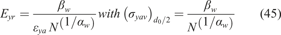
The stiffness of the 0° plies changes every time the plastic zone fails. The stiffness in the 90° plies on the other hand changes with every cycle, as can be inferred from equation (45), so “90° cycle blocks” or arbitrary number of cycles can be selected as long as they are shorter in duration than the 0° cycle block which fails the plastic zone. This way, when the end of a 0° ply block is reached, the stiffness of the 0° plies can be changed using the most up-to-date damage (and stiffness) state of the 90° plies. The residual stiffness of the 90° is updated at each block, together with the resulting laminate stiffness and applied strain. This allows the stress used in the 0° ply for the next 0° cycle block to be updated to account for all damage present in the 90° and 0° plies at the instant that the inter-fibre crack grows and the new plastic zone is formed.

The stress amplitude in the 0° plies is held constant throughout each 0° cycle block even when the stiffness of the 90° plies is changing. The effect of this simplifying assumption should be negligible, since for lower cyclic loads the stiffness of the 0° plies will barely degrade over the entirety of fatigue life, while for higher loads, the 90° plies will lose most of their stiffness immediately and keep losing the rest more gradually. In addition, the 0° cycle blocks for higher loads (where damage in the 0° plies drives laminate stiffness degradation) have the plastic zone growing every few cycles and thus the 0° cycle blocks are short enough to minimize the effect of this assumption. If cracks have formed in the 90° plies during the first cycle, their presence should be accounted for when using equation (45) to predict the residual stiffness in the 90° plies, since they will slow down the appearance of additional cracks. This is done by not allowing any further cracking (stiffness degradation) in the 90° plies until the number of cycles N representative of the first-cycle damage state has been applied. This number is obtained from equation (44) where (σ_yav)_do/2 is the average tensile stress between matrix cracks after the first cycle, determined in ref. 45.

It should be noted that the model at this stage neglects the fact that transverse cracks in a 90 °ply can cause fibre cracks in the 0° plies (and delaminations at 0/90° ply interfaces). This can be of significance when the first cracks in the 90° plies are created which have irregular crack spacing. This is a topic for future extensions of the model. For higher applied loads or number of fatigue cycles, the spacing of matrix cracks in the 90° plies and fibre cracks in the 0° plies become more uniform and the model can be used as presented above.

The approach just described was applied to a [0/90₂]s graphite/epoxy laminate to determine axial stiffness as a function of cycles for three different applied loads: 85%, 53% and 28% of the static failure strength of 779 MPa⁴⁷ with R = 0.1. The predictions are compared to test data from.⁴⁸ The material is AS4/3501-6 with mean Y_is^t = 49.31 MPa⁴⁸ and coefficient of variation of 12.1%.³⁷ After adjusting for R = 0.1,³⁵ the resulting Weibull distribution has shape and scale parameters of 11.34 and 55.23 MPa respectively. The predictions from the present method are compared to the test results in ref. 48 in Figure 14.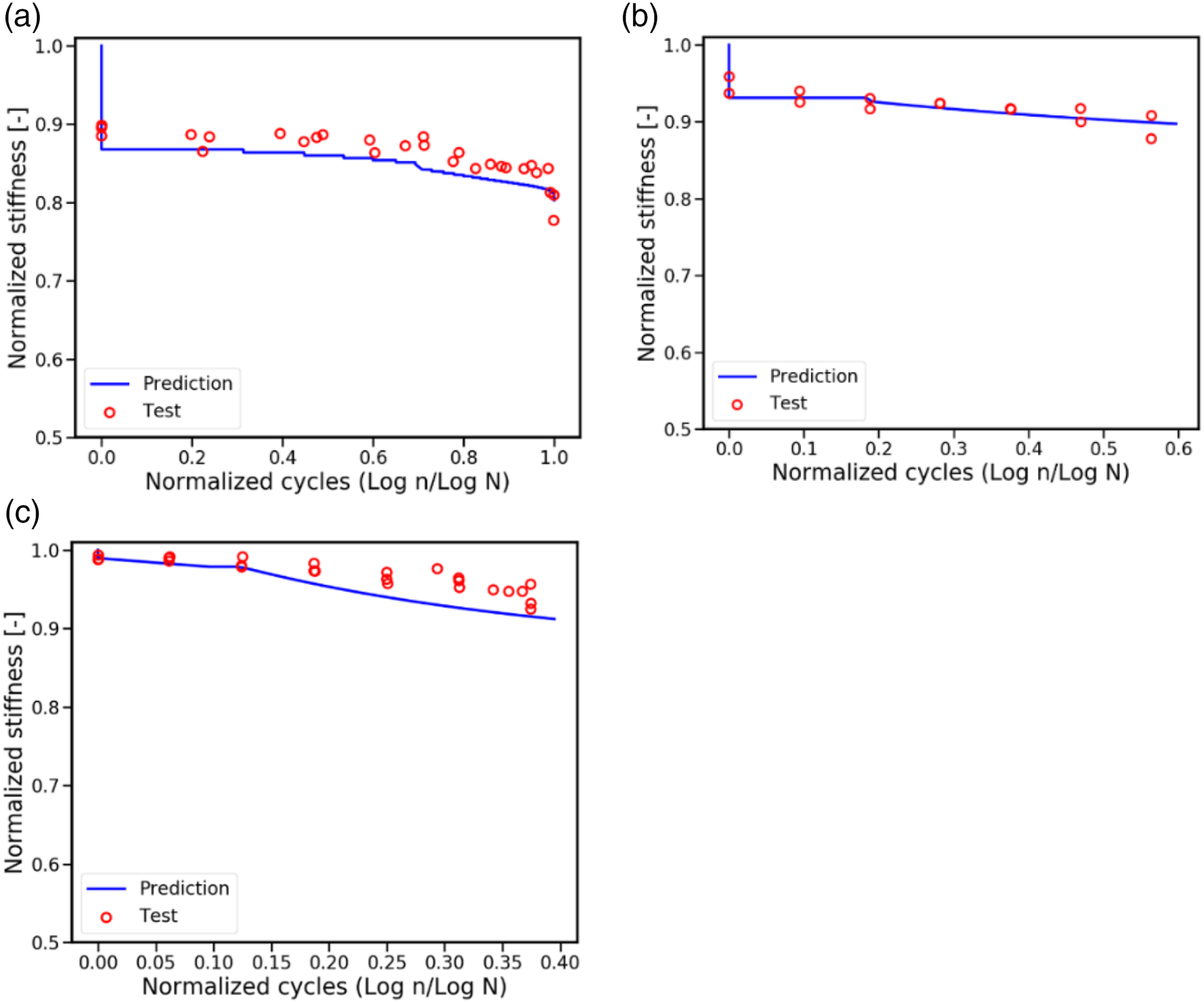

Figure 14.

Predicted laminate stiffness degradation as a function of cycles compared to tests from.⁴⁸ (a) Applied stress = 85% of static strength. (b) Applied stress = 53% of static strength. (c) Applied stress = 28% of static strength.

In Figure 14, consistent with how the results were presented in ref. 48 the x axis has the ratio of the logarithm of the cycles divided by the logarithm of the cycles to failure. Note that in Figures 14(b) and (c) the test data stop before final failure and, hence, the x axis does not extend to the value of 1. For the cycles to failure, the life predicted by the present method with inter-fibre cracks in the 0° plies reaching the center of the nearest fibre was used. It can be seen from Figure 14 that the predictions are in excellent agreement with test results and only for the 28% applied load case, Figure 14(c), the predictions are slightly conservative. It should be pointed out that the present method accurately predicts the initial steep drop of stiffness for the 85% and 53% load cases and shows only a gradual stiffness drop for the first few cycles for the 28% in very good agreement with the test results. It should be noted that, at this stage of its development, the present method does not account for delaminations. In these tests, delaminations were reported towards the end of life and there are plans to include them in future work.

Discussion and conclusions

The stresses in the matrix near the crack tip of a cracked fibre were determined with a new formulation. They were used in an energy criterion for fracture to determine if cracks will grow parallel to the fibres or radially between fibres. It was shown that, for typical fibre volume fractions used in practice, radial matrix cracks are the preferred method for energy dissipation. The size of these cracks and the fraction of cracked fibres were used along with individual stiffness and strength properties for the fibre and matrix to predict failure of uni-directional tape composites under tension and were shown to be in good to excellent agreement with tests. Combined with previously developed models for matrix cracks in cross-ply laminates⁴⁵ and fatigue life predictions,³⁵ and accounting for the creation and growth of a plastic zone at the tip of the radial inter-fibre cracks, predictions for the fatigue life and stiffness degradation as a function of cycles for uni-directional and cross-ply laminates were obtained and shown to be in very good agreement with tests.

While the approach presented here is very promising, there are several assumptions and simplifications that need revisiting: First, the failure model implicitly requires that, at higher applied strains, cracks in fibres align, i.e. the crack spacing is small enough and a matrix crack growing from one fibre will, at some point, line up with a crack growing from a neighbouring fibre. Second, the interaction between damage created in 0° and 90° plies is mainly accounted for by updating the stiffness properties in each ply. This is a simplification which does not account for the fact that at the tip of a crack in a 90° ply, stress is transferred from that ply to adjacent 0° plies locally changing the stress field. While this change is small at low loads, at higher loads it can affect the creation of fibre cracks in the 0° plies and lead to earlier failure. Third, the model used to determine crack opening displacement, crack length and plastic zone size is based on the Nied-Erdogan solution in ref. 23 which does not include the additional bending moment that the loaded fibre exerts to the surrounding matrix. This bending moment is relatively small for higher fibre volume fractions but may become significant at lower fibre volume fractions. In addition, the Nied-Erdogan results were extrapolated here in a few cases where the crack lengths were longer than the tabulated results in ref. 23 would allow. Also, determining the plastic zone size using a stress intensity factor from linear elastic fracture mechanics is an approximation which could be improved. Fourth, the model for cracks growing in the plastic zone ahead of a radial matrix crack does not account for any dynamic effects and does not include any retardation and crack path changes that will occur as the crack approaches a neighbouring locally intact fibre which has higher stiffness and fracture toughness than the matrix. This may explain why the predictions in Figure 11 are conservative, especially for high cycle fatigue.

Footnotes

Declaration of conflicting interests

The author(s) declared no potential conflicts of interest with respect to the research, authorship, and/or publication of this article. The Authors declare that there is no conflict of interest.

Funding

The author(s) received no financial support for the research, authorship, and/or publication of this article. This research received no specific grant from any funding agency in the public, commercial, or not-for-profit sectors.

ORCID iDs

Carlo Alberto Socci

Christos Kassapoglou

References

Degrieck

Van Paepegem

. Fatigue damage modeling of fibre-reinforced composite materials: review. Appl Mech Rev 2001; 54(4): 279.

Passipoularidis

Brøndsted

. Fatigue evaluation algorithms: review. Risø-R-Reports 1740, 2009.

Whitworth

. A stiffness degradation model for composite laminates under fatigue loading. Compos Struct 1998; 40(2): 95.

Yang

Lee

Sheu

. Modulus reduction and fatigue damage of matrix dominated composite laminates. Compos Struct 1992; 21: 91–100.

Talreja

. A continuum mechanics characterization of damage in composite materials. Proc R Soc Lond Ser A, Math Phys Sci 1985; 399: 195–216.

Talreja

. Stiffness properties of composite laminates with matrix cracking and interior delamination. Eng Fracture Mech 1986; 25(5–6): 751–762.

Aboudi

Lee

Herakovich

. Three-dimensional analysis of laminates with cross-cracks. J Appl Mech 1988; 55(2): 389–397.

Van Paepegem

De Baere

Lamkanfi

, et al. Monitoring quasi-static and cyclic fatigue damage in fibre-reinforced plastics by poisson’s ratio evolution. Int J Fatigue 1990; 32(1): 184.

Berthelot

Le Corre

. Modelling the transverse cracking in cross-ply laminates: application to fatigue. Compos B: Eng 1999; 30: 569–577.

10.

Montesano

McCleave

Veer Singh

. Prediction of ply crack evolution and stiffness degradation in multidirectional symmetric laminates under multiaxial stress states. Compos B: Eng 2018; 133: 53–67.

11.

Shokrieh

Lessard

. Progressive fatigue damage modeling of composite materials, part I: modeling. J Compos Mater 2000; 34.

12.

Ladeveze

Le Dantec

. Damage modelling of the elementary ply for laminated composites. Compos Sci Technol 1992; 43: 257–267.

13.

Maimí

Camanho

Mayugo

, et al. A continuum damage model for composite laminates. Part I: constitutive model. Mech Mater 2007; 39: 897–908.

14.

Breite

Melnikov

Turon

, et al. Detailed experimental validation and benchmarking of six models for longitudinal tensile failure of unidirectional composites. Compos Struct 2022; 279: 114828.

15.

Bonora

La Barbera

Marchetti

, et al. Experimental verification and theoretical simulation of fracture behaviours of composite materials. Compos Struct 1993; 23(2): 87–97.

16.

Mohammadi

Pakdel

. Materials & design fatigue driven matrix crack propagation in laminated composites. Mater Des 2018; 146: 108–115.

17.

Gamstedt

Ӧstlund

. Fatigue propagation of fibre-bridged cracks in unidirectional polymer-matrix composites. Appl Compos Mater 2001; 8: 385–410.

18.

Gamstedt

Talreja

. Fatigue damage mechanisms in unidirectional carbon-fibre-reinforced plastics. J Mater Sci 1999; 34: 2535–2546.

19.

Cox

. The elasticity and strength of paper and other fibrous materials. Br J Appl Phys 1952; 3(3): 72.

20.

Nairn

. On the use of shear-lag methods for analysis of stress transfer in unidirectional composites. Mech Mater 1997; 26: 63–80.

21.

Nairn

. Generalized shear lag analysis including imperfect interfaces. Adv Compos Lett 2004; 13: 263–274.

22.

Sørensen

. Micromechanical model of the single fibre fragmentation test. Mech Mater 2017; 104: 38–48.

23.

Nied

Erdogan

. The elasticity problem for a thick-walled cylinder containing a circumferential crack. Int J Fracture 1983; 22: 277–301.

24.

Budiansky

Hutchinson

Evans

. Matrix fracture in fibre reinforced ceramics. J Mech Phys Sol 1986; 34(2): 167–189.

25.

Huo

Kassapoglou

Alderliesten

. A criterion for predicting delamination growth in composite laminates. Mater Des; 223: 2022.

26.

Esrail

Kassapoglou

. An efficient approach for damage quantification in quasi-isotropic composite laminates under low speed impact. Compos B: Eng 2014; 61: 116–126.

27.

Kim

Nairn

. Observations of fibre fracture and interfacial debonding phenomena using the fragmentation test in single fibre composites. J Compos Mater 2002; 36: 1825–1858.

28.

Kaddour

Hinton

Smith

, et al. Mechanical properties and details of composite laminates for the test cases used in the third world-wide failure exercise. J Compos Mater 2013; 47: 2427–2442.

29.

Greenfield

Pedicini

Penn

. Development of a single fibre fragmentation test for high strain rates. Int J Adhes Adhesives 2000; 20: 403–407.

30.

Qian

. Multi-scale modelling of fatigue of wind turbine rotor blade composites. PhD thesis. Delft, Netherlands: Dept of Aerospace Engineering, Delft University of Technology, 2013. chapter 3.

31.

Huang

Talreja

. Numerical simulation of matrix micro-cracking in short fibre reinforced polymer composites: initiation and propagation. Compos Sci Tech 2006; 66: 2743–2757.

32.

Sjögren

Joffe

Berglund

, et al. Effects of fibre coating (size) on properties of glass fibre/vinyl ester composites. Composites A Applied Sci Manufac 1999; 30: 1009–1015.

33.

Zhuang

Talreja

Varna

. Tensile failure of unidirectional composites from a local fracture plane. Compos Sci Tech 2016; 133: 119–127.

34.

Qian

Westphal

Kassapoglou

, et al. Development of a multi-fibre unit cell for use in modelling of fatigue of unidirectional composites. Compos Struct 2013; 99: 288–295.

35.

Kassapoglou

. Fatigue life prediction of composite structures under constant amplitude loading. J Compos Mater 2007; 41: 2737–2754.

36.

Sørensen

Goutianos

Mikkelsen

, et al. Fatigue damage growth and fatigue life of unidirectional composites. Compos Sci Tech 2021: 211: 108656.

37.

Composite materials handbook, MIL-HDBK-17-2F, vol 2 Polymer Matrix Composites Material Properties, 1999, ch 4.

38.

Kassapoglou

. Fatigue model for composites based on the cycle-by-cycle probability of failure: implications and applications. J Compos Mater 2011; 45(3): 261–277.

39.

Mishra

El-Hajjar

. Non-linear strain invariant failure approach for fibre reinforced composite materials. Int J Mater Struct Integrity 2012; 6: 284–296.

40.

Odom

Adams

. An investigation of the isotropy of epoxy polymers. J Mat Res 1992; 7(12): 3352–3358.

41.

Lee

Daniel

Yaniv

. Fatigue life prediction of cross-ply composite laminates. In: Lagacé

(ed). Composite materials: fatigue and fracture. ASTM STP 1012, 2nd ed. Philadelphia, USA: American Society for Testing Materials, 1992, pp. 19–28.

42.

Reifsnider

Schulte

Duke

. Long-term fatigue behaviour of composite materials. In: O’Brien

(ed). Long term behaviour of composites, ASTM STP 813. Philadelphia, USA: ASTM Philadelphia, 1983, pp. 136–159.

43.

Charewicz

Daniel

. Damage mechanisms and accumulation in graphite/epoxy laminates. In: Hahn

(ed). Composite materials: fatigue and fracture, ASTM STP 907. Philadelphia, USA: ASTM, 1986, pp. 274–297.

44.

Simonds

Bakis

Stinchcomb

. Effects of matrix toughness on fatigue response of graphite fibre composite laminates. In: Lagacé

(ed). Composite materials: fatigue and fracture, ASTM STP 1012. Philadelphia, USA: ASTM, 1989, Vol. 2, pp. 5–18.

45.

Socci

Kassapoglou

. Prediction of matrix crack initiation and evolution and their effect on the stiffness of laminates with off-axis plies under in-plane loading. Compos Sci Tech 2020: 200: 108427.

46.

Ryder

Crossman

. A study of stiffness, residual strength and fatigue life relationships for composite laminates. Rep NASA CR 172211; 1983.

47.

Daniel

Lee

. Damage development in composite laminates under monotonic loading. J Composites Tech Res 1990; 12(2): 98–102.

48.

Daniel

Lee

Yaniv

. Damage mechanisms and stiffness degradation in graphite/epoxy composites. In: ICCM and ECCM (Sixth International Conference on Composite Materials and Second European Conference on Composite Materials), London, UK, 1987; 4: 129–138.

Effect of matrix and fibre cracks on static and fatigue strength of composite laminates

Abstract

Keywords

Introduction

Approach

Strength and stiffness of a 0° unidirectional tape ply

Stress field around fibre crack

Fibre/matrix interface crack

Inter-fibre radial matrix crack

Fibre/matrix cracks versus inter-fibre radial matrix cracks

Stiffness of a 0° uni-directional ply after fibre cracking

Strength of a 0° uni-directional ply

Extension to fatigue

Fatigue of 0° ply

Fatigue of 90° ply

Fatigue of cross-ply laminates

Discussion and conclusions

Footnotes

Declaration of conflicting interests

Funding

ORCID iDs

References