Sage Journals: Discover world-class research

Abstract

Extrinsic toughening, such as fibre bridging, acts behind the crack tip to increase toughness in composite laminates. Computational studies have captured this phenomenon; however, the uniqueness of fit between computational results (which vary based on the interface traction-separation relationship) and experimental results has not been explored in detail. Here, detailed exploration of the parameter space for various traction-separation laws (TSL) using finite elements is presented to investigate the role of fibre bridging. In the absence of extrinsic toughening, a linear softening TSL is sufficient to capture the key R-curve features, the total input fracture energy is of primary importance. Where extrinsic toughening is present, the ratio between intrinsic and extrinsic energy dictates the shape of the crack growth resistance curve (where fracture toughness (energy) increases with increasing crack growth). The influence of fibre bridging length on the crack growth required to reach a plateau in toughness is examined. A strategy for determining key cohesive properties from a double cantilever beam test is presented and applied to experimental results.

Keywords

composite laminate double cantilever beam test extrinsic toughness fibre bridging finite element interlaminar failure traction separation law

Introduction

Composite materials composed from stacked layers of continuous fibres embedded within a polymeric matrix provide high specific strength and stiffness properties. As such, composites find increasing use in aircraft structures, automotive components, and wind turbine blades. A direct consequence of motion is a greater susceptibility to impact loads; if the application includes a cyclical element, fatigue life can also be of concern. Both impact and fatigue can result in delamination between the stacked layers of the composite. Both intrinsic and extrinsic toughening mechanisms (which act ahead of the crack tip and behind the crack tip, respectively, as seen in Figure 1(a)) influence the onset and progression of failures.^1–3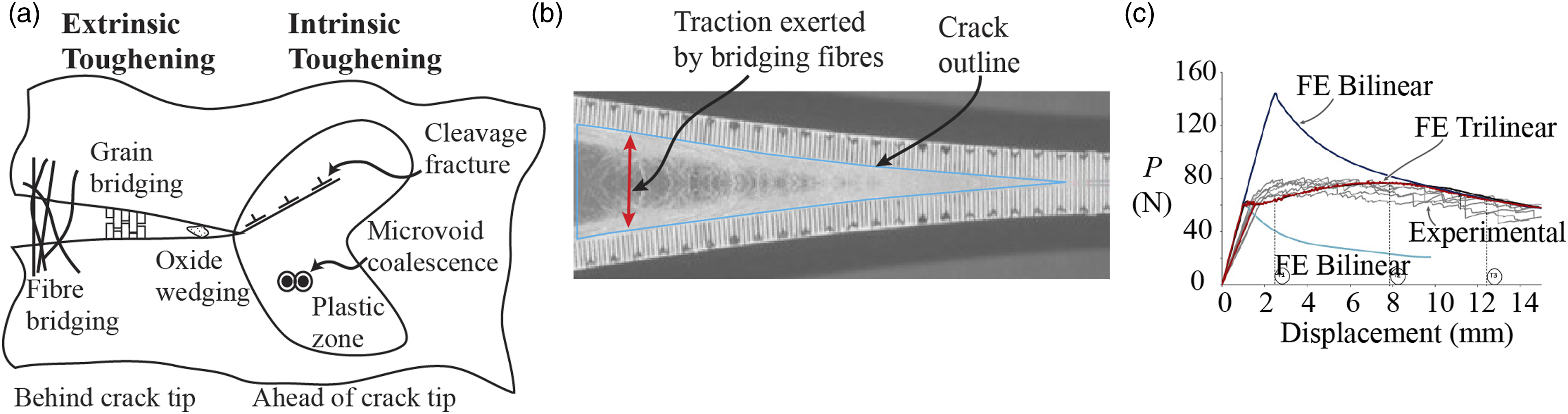

Figure 1.

(a) Examples of extrinsic and intrinsic toughening mechanisms. Image adapted from Liu et al.²⁸ (b) Example of fibre bridging in GFRP.²¹ (c) Experimental load-displacement behaviour replicated computationally.²⁹

Intrinsic and extrinsic toughening

Intrinsic toughening mechanisms act ahead of the crack tip and extrinsic toughening mechanisms act behind the crack tip (see Figure 1(a)); however, the definition of the crack tip can vary significantly. The terms ‘damage’ and ‘toughening’ can describe the same phenomena depending on the crack tip definition.⁴ Sills and Thouless also suggest that a change in cohesive length scale can be used to define the transition from intrinsic to extrinsic toughening.⁴

The role of intrinsic toughening mechanisms in traditional engineering materials is well studied, for example, micro-matrix cracking.⁵ Other examples of intrinsic mechanisms include: plasticity ahead of a crack tip in steels and other ductile metals,^6,7 crack deflection by secondary phases⁸; crack bifurcations⁹ and void coalescence.¹⁰ In composites, the intrinsic toughness is dictated by the resin properties,¹¹ fibre volume fraction,¹² and the mean fibre diameter.¹³

Extrinsic toughening mechanisms act behind the crack tip to increase fracture toughness (Figure 1(a)). Of particular relevance to composite materials is fibre bridging (shown in Figure 1(b)), an extrinsic toughening mechanism whereby fibres from neighbouring plies remain attached to both delaminated layers. This generates a traction across the crack and, hence, raises the energy required to advance the crack front. This effect can act over a large separation, as found in Carbon Fibre Reinforced Polymers (CFRP) composites,¹⁴ or a short separation, as found in biological tissue.¹⁵ Fibre bridging acting over a seemingly short distance still significantly affects the evolution of fracture toughness. In mode I or mixed-mode loading.^16–18 Typical experimental results in the presence of fibre bridging, show a less obvious peak in the load-displacement response (Figure 1(c)).; The role fibre bridging plays in crack deflection is difficult to replicate computationally as discussed below.

Fibre bridging is of interest in engineered composite materials^14,19 as the additional extrinsic toughening, which may be fully realised under impact loading and subsequent delamination, could be the deciding factor between a destructive brittle failure and a controlled ductile failure. Fibre bridging has been characterised in composites such as CFRP,²⁰ Glass Fibre Reinforced Polymers (GFRP)²¹ and other fibre-rich epoxies.²² Fibre bridging also occurs in a range of biological and natural materials such as fibrous biological or natural materials (e.g. Liver tissue,²³ adipose tissue,²⁴ frozen arteries²⁵ and the cornea¹⁵ and timbers^26,27).

Experimental fracture tests with fibre bridging

The effect of fibre bridging is observed experimentally via the monotonic increase in fracture toughness or energy release rate with increasing crack length, shown in Figure 2(c). As an inter-laminate crack propagates in a DCB, the bridging fibres exert tractions on the delaminating surfaces, arresting the crack propagation. The initial value in the crack growth resistance (or R-curves), is set by the energy required for crack initiation. The energy required to advance the crack front increases as the amount of fibre bridging increases. The fracture toughness plateaus once new fibres bridging the interface compensate fibre breakage or fibre pull out at the other end of the crack and a steady-state turnover of fibres occurs.

Figure 2.

General shape of a traction-separation law. (a) Bilinear curve without fibre bridging present. (b) Trilinear curve with fibre bridging present. In the case of fibre bridging 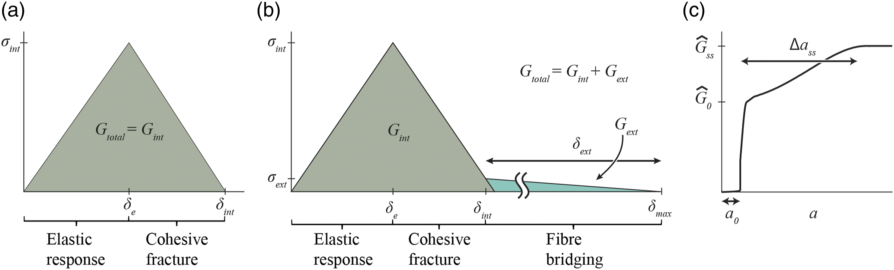$δ_{ext} ≫ δ_{e,} δ_{int}$ and diagram is not to scale (c) Idealised experimental observation of crack growth resistance showing key quantities.

Double cantilever beam (DCB) fracture tests of continuous fibre composites often exhibit fibre bridging.¹⁹ Typically, DCB experiments measure load, load-line displacement, and crack propagation and are used to produce crack growth resistance curves for a given material. DCB tests are most commonly performed in accordance with ASTM standards.³⁰ Four methods of data analysis are outlined in the standards: beam theory, modified beam theory, the compliance calibration method, and the modified compliance calibration method. The compliance calibration method is used in the present work and also, for example, Davidson and Waas.³¹ Compact tension shear type specimens are also used to investigate interlaminar fracture³²; however, generating a specimen of sufficient height involves a large number of laminates or compound specimens where the fibre composite is bonded to other materials. Other geometries, such as three-point bend tests can also test the interlaminar properties, although this also requires more complicated specimen fabrication.³³ In the current study, we focus on the DCB test specimen which consists of only the fibre composite.

Fibre bridging is observed experimentally via the monotonic increase in fracture toughness or energy release rate with increasing crack length, the so-called resistance curve (or R-curve), shown in Figure 2(c). Fibre bridging depends on the composite’s constituent materials and specimen geometry.^21,29,34 On initiation, the fracture toughness is exclusively determined by the intrinsic mechanisms. However, as the crack front advances, fibre bridging develops in its wake, and the observed fracture toughness increases monotonically as the contribution from bridging increases. The fracture toughness plateaus, reaching a steady state once a steady distribution of bridged fibres is created behind the crack tip. The key features of an R-curve are: the initial value of fracture toughness ${\hat{G}}_{0}$ , the plateaued value of fracture toughness ${\hat{G}}_{s s}$ , the initial crack length $a_{0}$ , and the length of the new crack surface created while achieving a steady state fracture toughness measurement $Δ a_{s s}$ as illustrated in Figure 2. Heidari-Rarani et al. model unidirectional DCB specimens under large-scale fibre bridging and experimental results show that the rise in the R-curve (from ${\hat{G}}_{0}$ to ${\hat{G}}_{s s}$ ) corresponds with the length of the process zone (which is defined by Heidari-Rarani et al. in their work as the distance between (i) the point where bridging and the fracture process initiate and (ii) the first point in the wake of damage zone that is unable to sustain cohesive tractions).²²

Data analysis

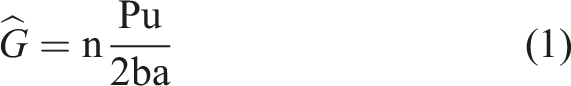
Using the compliance calibration method (as described in the ASTM standard), the fracture toughness $\hat{G}$ is determined from the applied load $P$ , the load-line displacement $u$ and the current crack length $a$ :

\hat{G} = n \frac{Pu}{2 ba}

(1)

where

b

is the specimen thickness, and

n

is a linear regression fitting parameter relating the compliance (

C = u / P

) to the crack length.³⁰ This regression parameter accounts for beam rotations at the crack tip. In DCB tests, measured load-displacement response and R-curves are dependent on the choice of certain material and specimen parameters, such as laminate thickness, modulus, and pre-crack length. Shokrieh et al. investigated the effect of initial crack length on unidirectional glass/epoxy DCB specimens.³⁴ While the values of

\hat{G}

do not vary with specimen, the crack length for each value does. It was found experimentally that the initial crack length

a_{0}

only slightly affects the shape of the response. Gutkin et al. also conducted a coupled experimental and computational study showing that an R-curve is dependent on thickness of the lever arm.²⁹

Determining cohesive properties

Experimental research on fibre bridging is often coupled with a model of the experimental procedure. In computational models of fibre bridging, it is necessary to formulate the appropriate traction-separation law (TSL), which is also referred to as a cohesive zone model (CZM). The TSL describes the traction exerted between two debonding surfaces at each point on the crack face based on the local separation between the surfaces. The integral of the function is the work done to fracture. Many studies consider the bridged fibres in this manner, i.e. not as discrete fibres in the model geometry; however, there has not been an in-depth systematic exploration of the influence of TSL parameters.

The shape of the TSL (typical examples are shown in Figure 2(a) and (b)) is critical in determining and the load-displacement response and the R-curve that will be produced by the simulation. There are several TSL shapes explored in the literature including trapezoidal,³⁵ bilinear,¹⁴ trilinear¹⁷ and a continuous function.^34,36 It has been found that a bilinear TSL (Figure 2(a)) is only able to capture the initial stages of fibre bridging^19,29,31 as shown in blue in Figure 1(c); whereas a trilinear law (Figure 2(b)) is capable of capturing high levels of separation typically found with fibre bridging^19,34,37 as shown in red in Figure 1(c). Intrinsic toughening mechanisms are collectively captured in the cohesive fracture zone of the TSL (as shown in Figure 2), which acts over short separations.

Figure 2 shows the general form of the traction-separation laws and establishes the terminology used in the current work (for use with the finite element method). For clarity, all fracture energies pertaining to the traction-separation laws are denoted by $G$ with various subscripts and all measured/observed (either experimentally or in the simulations) quantities are denoted by a circumflex, i.e. $\hat{G}$ . The fracture energy $G_{t o t a l}$ , is the total area under the TSL. This fracture energy can be split into intrinsic and extrinsic contributions, related to the respective toughening mechanisms, and can also be determined as the areas of the respective regions:

G_{i n t} ≅ \frac{1}{2} σ_{i n t} δ_{i n t}

(2)

G_{e x t} ≅ \frac{1}{2} σ_{e x t} δ_{e x t}

(3)

where all symbols are defined in Figure 2. Note that there is a small area overlap in equations (2) and (3), as

G_{t o t a l} \neq G_{i n t} + G_{e x t}

. The size of the area which is included in both the definition of

G_{i n t}

and

G_{e x t}

is equivalent to

\frac{σ_{e x t}}{σ_{i n t}} (δ_{i n t} - δ_{e})

. This value typically accounts for less than 1% of the total fracture toughness in the analyses considered.

While numerous studies have coupled experimental and computational work,^19,31,34,38 there is no simple procedure to select cohesive parameters for a finite element model based on experimental observations. In many studies, the J-integral method³⁹ is used to determine a TSL for laminates as part of a theoretical analysis^40,41 or numerical study.²² The J-integral method has also been used in ceramic composites⁴² and for coatings.⁴³ In most applications of the J-integral approach, the stresses on the crack surface are assumed to be zero and this is not true in the case of fibre bridging. In a series of works, Sørensen et al.^40,44 apply the J-integral method to fibre bridging to determine the cohesive law; but the loading of the specimen is via end moments.⁴⁵

Previous studies of crack growth in fibre composites have found that computational results can replicate the results in an experimental procedure with fibre bridging present.^{19,21,29,31,37,46} However, the effect of the input parameters on the fit between numerical and experimental results has not been explored and documented; the dominant parameters governing the observed phenomena are not described. Although for example, Heidari-Rarani et al. details their justification for a maximum traction $σ_{i n t}$ for different cases,²² no algorithm to fully define a TSL based on experimental observations is available. Dávila et al.⁴⁷ present an approach to determine fracture properties for a tri-linear TSL for a compact tension (CT) fracture specimen. Their approach superimposes two cohesive elements, each with linear softening and the same separation for the maximum traction. In this way, two triangular areas are superimposed, and the intrinsic and extrinsic toughness can be related to these areas and the ratios of the peak strengths and total energy for each element. However, this approach requires non-standard implementation in a finite element package, and they do not fully explore the sensitivity of the overall response to each of the input parameters. The present work provides an insight into selecting cohesive parameters for a TSL with extrinsic toughening based on experimental observations, via a systematic exploration of the TSL parameter space. Key relationships are presented and an approach to reconstruct a TSL based on a small set of experimentally observed variables is described. Several case studies are used to demonstrate the approach.

Modelling approach

Finite element model

Finite element models of a typical DCB fracture toughness test geometry, in line with ASTM standards,³⁰ are created in Abaqus version 6-14 (Dassault Systèmes, Rhode Island, USA, 2014) using 2D plane strain elements to represent the beams and the interfacial behaviour is captured using cohesive elements (shown in Figure 3). The mesh used is highly structured, consisting of square elements and the element size is determined by the height of a laminate arm; such that 25 elements are present along the vertical dimension of the laminate arm. A TSL is used to define behaviour of the cohesive layer. The response of the cohesive element follows the default behaviour, whereby the strain is equivalent to the displacement as a unit thickness is used in the material calculation. Although the height of the cohesive layer does not affect the response, the nodes in the cohesive layer are adjusted so that the layer has geometrically zero thickness in the y-direction.⁴⁸

Figure 3.

(a) FE model geometry, based on (b) a typical composite test specimen with loading blocks in compliance with ASTM standards.³⁰

The features of the ASTM standard DCB test are captured in the finite element model: the loading blocks are represented by using the Coupling Constraint method and displacements are applied to the associated reference points (with resulting reaction forces). For simplicity, and in line with previous studies of crack growth in CFRP,¹⁹ the laminate properties used in this model are isotropic linear elastic with Young’s modulus of 170 GPa and Poisson ratio of 0.3 unless otherwise stated. As the transverse behaviour is not relevant to the investigations (as only axial stretching is considered for simplicity), the laminates are modelled as isotropic; however, the methodology can be applied to anisotropic laminates. The isotropic nature of these models allows the results to be applied to other materials with in-plane isotropic properties.

The load-displacement response is measured at the upper reference point, Figure 3(a). The fracture toughness is calculated by the compliance calibration method.³⁰ Definition of the crack tip can be difficult and somewhat arbitrary when fibre bridging is present. The crack tip can be defined by observation or using the beam compliance. Difficulty arises in experimental observations due to extrinsic toughening mechanisms obstructing the view of the crack tip. In this study, the crack length is defined as the distance from the pre-crack to where the separation of the surfaces is equal to $δ_{e}$ (as defined in Figure 2). As this study is computational, a separation of $δ_{e}$ can be measured in postprocessing to identify the crack tip; in practice measuring this separation (of $δ_{e}$ ) is not simple. The crack length measurement is used in equation (1) to produce the R-curve.

A TSL is shown in Figure 2 where the traction in a cohesive element $σ$ is defined in terms of the local separation $δ$ . The shape of the curve is defined by an initial cohesive stiffness $k_{c}$ , a maximum traction $σ_{i n t}$ , and subsequent pairs of $σ$ and $δ$ which define the traction-separation response. In the current study, only mode I cracks are considered, and any tangential displacements are not considered.

The simulation is solved using a non-linear implicit scheme in Abaqus/Standard. The TSL is implemented in Abaqus by assigning the “traction-separation” section type to the cohesive layer; the initial stiffness is represented by an elastic constant and subsequent tractions are captured using the “damage initiation” and “damage evolution” options. The lower reference point is fixed in all translational degrees of freedom while being free to rotate, and the upper block is displaced vertically upwards. The displacement of this point $u$ , the resulting reaction force $P$ , and the crack length $a$ are recorded and used to calculate the measured fracture energy $\hat{G}$ using the same compliance calibration method as used in the ASTM experimental methods (equation (1)).

Parameter variation details

A systematic variation of the parameters associated with the TSL (governing the material behaviour of the interface) is conducted, along with specimen specific parameter variation. To represent intrinsic toughness only, it is sufficient to describe a TSL using $k_{c}$ , $σ_{i n t}$ , and $δ_{i n t}$ (note $δ_{e} = σ_{i n t} / k_{c}$ is not independent). Extrinsic toughening (bridging behaviour) is considered by using a TSL which includes tractions which act over larger separations; in the case of the tri-linear law, as shown in Figure 2(b), two extra parameters $δ_{e x t}$ and $σ_{e x t}$ are required.

For intrinsic toughness only, a wide range of TSL parameters $(δ_{e}, δ_{i n t}, σ_{i n t})$ and TSL shapes (bi-linear and trapezoidal) are considered and the details and results are shown in Appendix 1. In terms of the shape of the TSL, the energy, i.e. the area under the curve, dictates the observed response as longs as $δ_{i n t}$ is small. If $δ_{i n t}$ is too large, then the peak in the load-displacement response becomes less distinct and would not capture typical experimentally observed behaviour. The elastic loading slope and the softening/unloading slope will affect the computational cost, but uncertainty in the experimental data would frustrate any attempt at calibrating these values. Convergence issues occur and numerical noise is observable in the load-displacement response for $L_{e l} / δ_{i n t} \geq 50$ (data not shown) or if both slopes on the intrinsic region are not of similar magnitude; therefore, setting $δ_{e} = δ_{i n t} / 2$ is recommended. Estimation of $σ_{i n t}$ is discussed below in Section 3.4.

For materials with both intrinsic and extrinsic toughness, the parameter space is explored systematically in four phases I-IV (with the details in Tables 1, 2, and 3). The intrinsic toughness is not varied in these phases; the parameters relating to the intrinsic part of the TSL are fixed, unless otherwise noted; previous simulations of experimental data are used to determine appropriate ranges for parameters.¹⁹

Table 1.

Details of parameter variation I and II (examining the ratio of intrinsic to extrinsic toughness). This study has been completed for $σ_{ext} = 0.1, 0.4, 1.0 & 4.0$ MPa. All results show the same trend regardless of $σ_{ext}$ .

Phase	$σ_{int}$ $(MPa)$	$σ_{ext}$ $(MPa)$	$δ_{e}$ $(μm)$	$δ_{int}$ $(μm)$	$δ_{ext}$ $(mm)$	$G_{int}$ $(J / m^{2})$	$G_{ext}$ $(J / m^{2})$	$G_{total}$ $(J / m^{2})$
I	40	0.4	5	15	0.05	300	10	310
	40	0.4	5	15	0.1	300	20	320
	40	0.4	5	15	0.3	300	60	360
	40	0.4	5	15	0.5	300	100	400
	40	0.4	5	15	1.0	300	200	500
II	40	0.4	5	19.5	0.05	390	10	400
	40	0.4	5	19	0.1	380	20	400
	40	0.4	5	17	0.3	340	60	400
	40	0.4	5	15	0.5	300	100	400
	40	0.4	5	10	1.0	200	200	400

Table 2.

Summary of parameter variation III, examining R-curve specimen dependence, full list of parameter combinations is in the supplementary material.

Phase	Parameter	Values
III	$L$ (mm)	150, 300, 400, 600, 1,000
	$a_{0}$ (mm)	0, 10, 25, 50, 60, 70, 100
	$E$ (GPa)	50, 170, 300, 600, 1,000, 1,700
	$h$ (mm)	2, 3, 4, 5, 6, 7, 8, 12, 16

Table 3.

Values of $σ_{e x t}$ (MPa) for the shape variation of the extrinsic toughening region (phase IV). Intrinsic toughening properties are fixed. $δ_{e} = 0.005$ mm, $δ_{i n t} = 0.01$ mm, $σ_{int} = 40$ MPa, $G_{int} = 200 J / m^{2}$ .

		$δ_{ext} (mm)$	0.05	0.1	0.25	0.5	1	2.5	10
IV	$σ_{ext}$ (MPa)	$G_{ext} = 200 J / m^{2}$	8	4	1.5	0.8	0.4	0.16	0.04
		$G_{ext} = 400 J / m^{2}$	16	8	3.2	1.6	0.8	0.32	0.08
		$G_{ext} = 1000 J / m^{2}$	N/A	20	8	4	2	0.8	0.2
		$G_{ext} = 2000 J / m^{2}$	N/A	N/A	16	8	4	1.6	0.4

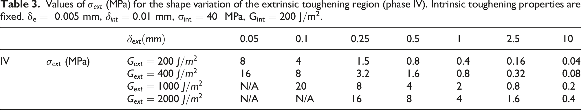
The four phases are:

I. The intrinsic properties $(σ_{i n t}, δ_{e}, δ_{i n t})$ are held constant and the extrinsic toughness $G_{e x t}$ is varied by increasing the bridging length $δ_{e x t}$ .

II. The total fracture energy $G_{t o t a l}$ is held constant but the ratio of $G_{i n t} : G_{e x t}$ is varied. This means that the elastic region $(σ_{i n t}, δ_{e})$ is constant but the cohesive fracture zone $(δ_{i n t}, σ_{e x t})$ is allowed to move to ensure the total energy $G_{t o t a l}$ remains constant across analyses.

III. The R-curve specimen dependence is examined by varying dimensions and modulus with fixed TSL parameters ( $δ_{e} = 0.005$ mm, $δ_{i n t} = 0.01$ mm, $δ_{e x t}$ = 1 mm, $σ_{i n t}$ = 40 MPa, $σ_{e x t}$ = 0.4 MPa, $G_{i n t} = 200 J / m^{2}$ and $G_{e x t} = 200 J / m^{2}$ ). Details are found in Table 2.

IV. The shape of the extrinsic region is varied by adjusting the extrinsic parameters ( $δ_{e x t}$ and $σ_{e x t}$ ) for constant extrinsic toughness. As the bridging length $δ_{e x t}$ increases, the bridging stress $σ_{e x t}$ decreases so that the extrinsic toughness stays constant. This is repeated for four values of $G_{e x t}$ as shown in Table 3.

Results

Figure 4 shows the deformed configuration of a DCB simulation with an intrinsic toughness of 300 $J / m^{2}$ and an extrinsic toughness of 200 $J / m^{2}$ (with properties as shown in the final row of Table 1 phase I and in Figure 4(b)). The cohesive tractions, shown as arrows in Figure 4(a) in the steady-state (i.e. once the measured toughness has reached a plateau), are at a maximum at the crack tip (defined here as $δ = δ_{e}$ ) and decrease monotonically in the bridging zone behind the crack tip. The approximate lengths over which the tractions act are shown in Figures 3 and 4 and identified by measuring the distance along the crack from where the separation is $δ = δ_{e} / 10$ to the peak in the traction curve (2 mm), from the peak to $δ = δ_{i n t}$ (1.7 mm), and from $δ = δ_{i n t}$ to $δ = δ_{m a x}$ (38 mm). The load versus load-line displacement (Figure 4(c)) shows a peak at which time crack propagation commences followed by a reduction in force as the crack grows as a result of the reduction in compliance of the DCB arms. The substantial amount of extrinsic fracture energy results in a rising R curve behaviour (Figure 4(d)); the initial value of the measured fracture energy is a direct result of the intrinsic toughness, and a final/plateaued value is determined by the total fracture energy (i.e. intrinsic plus extrinsic). The crack growth which occurs before the plateau is reached (and a steady-state toughness is obtained) is hereafter referred to as $Δ a_{s s}$ .

Figure 4.

(a) Deformed shape of DCB specimen with overlaid traction vectors. The dimensions of 2 mm, 1.7 mm and 38 mm show the differing crack length scales over which intrinsic and extrinsic toughening mechanisms act. Applied traction-separation law shown (b) with the measured load-displacement response (c) and resulting R-curve, normalised with input fracture energy 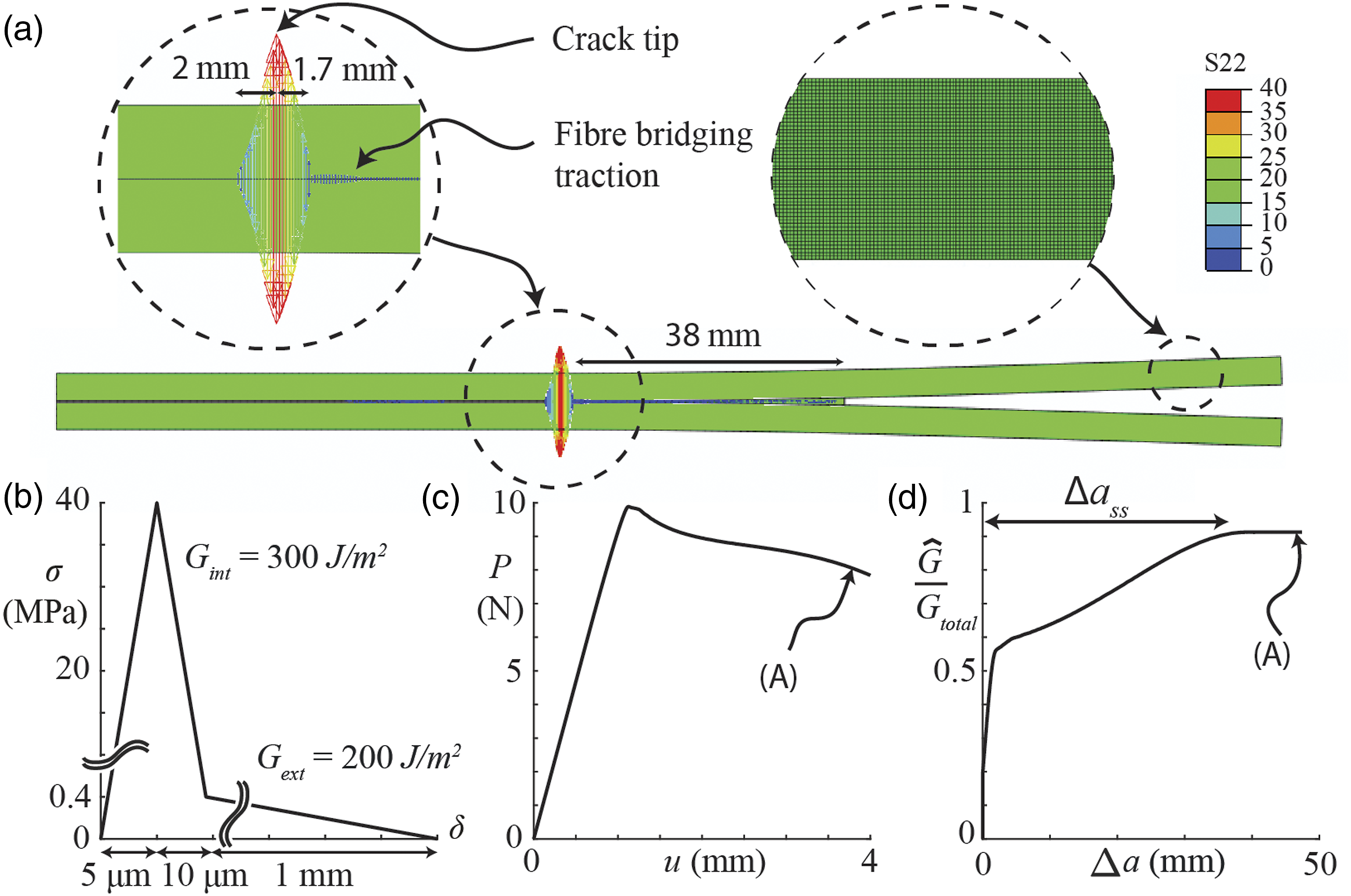$G_{total}$ (d).

The ratio of extrinsic to intrinsic toughness $(G_{ext} : G_{int})$

The effect of the ratio of intrinsic toughness to extrinsic toughness on the overall R-curve behaviour is summarised in Figure 5 based on the parameters listed above (I and II in Table 1). In the first set of results (Figure 5(a)–(d)), the intrinsic toughness is fixed and the extrinsic varied and, in the second (Figure 5(e)–(h)), the total toughness is fixed and the ratio of intrinsic to extrinsic toughening is varied. In the case of the former (Figure 5(a)–(d)), the following observations are made: (i) the peak load is constant, (ii) the crack growth length to reach the steady-state measured toughness $Δ a_{s s}$ increases with increasing $G_{e x t}$ , (iii) the plateau/steady-state measured toughness increases with $G_{t o t a l}$ , and (iv), when normalized by the total toughness, the steady-state measured toughness $\approx 1$ , as expected.

Figure 5.

Summarised input parameters and results from phase I (where 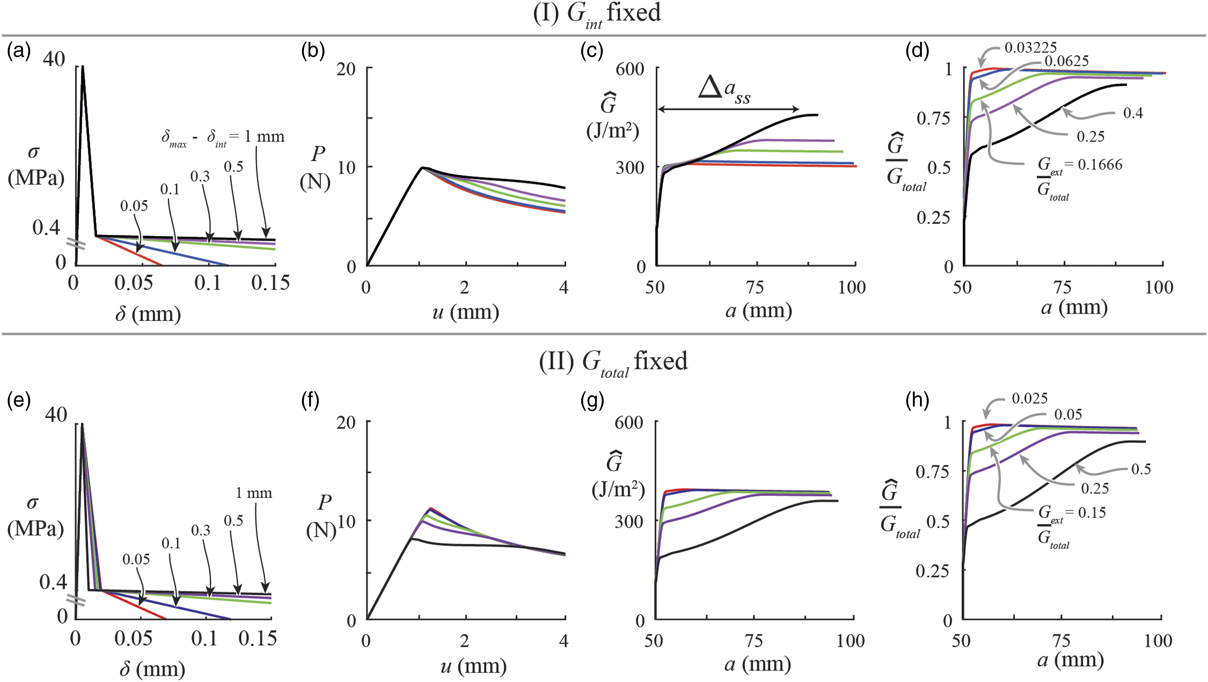$G_{i n t}$ is fixed and $G_{e x t}$ is varied) and II (where $G_{t o t}$ is fixed and the ratio of $G_{i n t} : G_{e x t}$ is varied) of the parameter variation, examining the ratio of intrinsic to extrinsic toughness.

In second set of results (Figure 5(e)–(h)), and similar to the above, we note: (i) the peak load increases with increasing $G_{i n t}$ , (ii) $Δ a_{s s}$ increases with increasing $G_{e x t}$ , and (iii) the plateau/steady-state measured toughness is constant with constant $G_{t o t a l}$ . In these simulations, the extrinsic energy is increased by increasing $δ_{e x t}$ and correspondingly, $δ_{i n t}$ is reduced to keep the total energy constant.

These results show that the R-curve behaviour is dominated by changes in the extrinsic toughness, as expected; however, in these simulations only $δ_{e x t}$ is varied. A further investigation of the other extrinsic parameters is shown below.

Effect of fracture test properties

In the current section, the effect of test specimen parameters ( $h$ , $E$ , $a_{0}$ ) on the response are explored (the series of simulations III in Table 2). Figure 6 shows that increasing $h$ (Figure 6(a)) or increasing $E$ (Figure 6(d)) causes an increase in $Δ a_{s s}$ . For a valid beam test (i.e. $\frac{a_{0}}{h} > 10$ ), $Δ a_{s s}$ is linearly proportional to $h$ for all values of $E$ considered (Figure 6(b) and (c)), as evident from the 1:1 relationship on a log-log scale indicating a linear relationship. Similarly, $Δ a_{s s}$ is linearly proportional to $\sqrt[3]{E}$ for all values of $h$ considered (Figure 6(e) and (f)), as evident from the 1:3 relationship on a log-log scale. The original crack length $a_{0}$ does not affect the behaviour for slender beams (data not shown).

Figure 6.

Top row: Relationship between steady-state crack growth 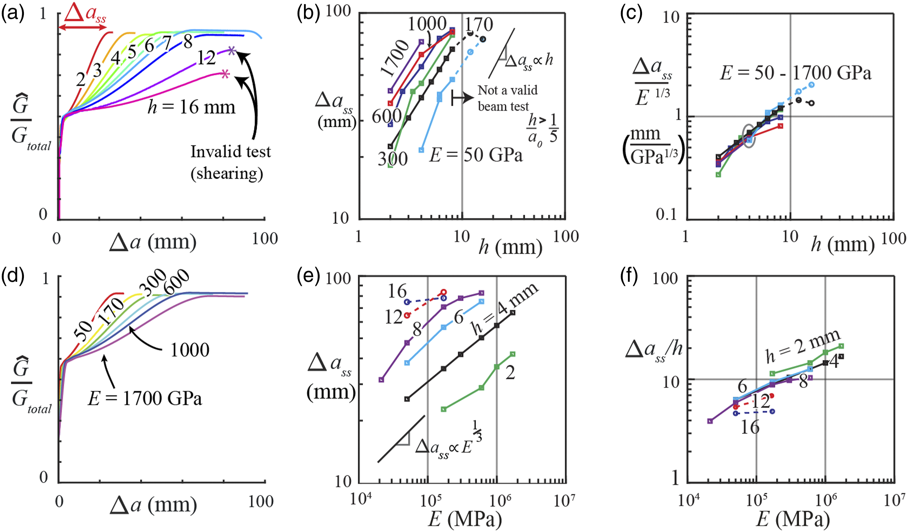${Δa}_{ss}$ and beam thickness $h$ for $E = 170 GPa$ (a) R-curves. (b,c) A linear relationship (note 1:1 relationship is also shown) between ${Δa}_{ss}$ and $h$ for various laminate moduli. Bottom row: Relationship between steady-state crack growth ${Δa}_{ss}$ and beam modulus $E$ for $h = 4 mm$ . (d) R-curves. (e,f) showing relationship between ${Δa}_{ss}$ and $E$ for various laminate thicknesses.

Bridging length and steady-state crack length

Previously, $G_{e x t}$ was shown to control the shape of the R-curve by varying $δ_{e x t}$ ; here we show the $G_{e x t}$ does not substantially change the ratio $Δ a_{s s} / δ_{e x t}$ . Therefore, the bridging length is the most important parameter––bridging tractions will influence the overall toughness, but not the slope of an R-curve ( $\hat{G} / G_{t o t a l}$ vs $Δ a$ ). A range of behaviours are considered ; within each group of simulations $δ_{e x t}$ is varied such that $G_{e x t} = 0.5 σ_{e x t} δ_{e x t}$ is constant (Figure 7(a)); this is repeated for 4 different values of $G_{e x t}$ in total (Table 3). For all values of $G_{e x t}$ , $Δ a_{s s}$ is shown to linearly increase with $δ_{e x t}$ . In all cases, $G_{i n t} = 200 J / m^{2}$ .

Figure 7.

(a) Traction-separation laws with constant 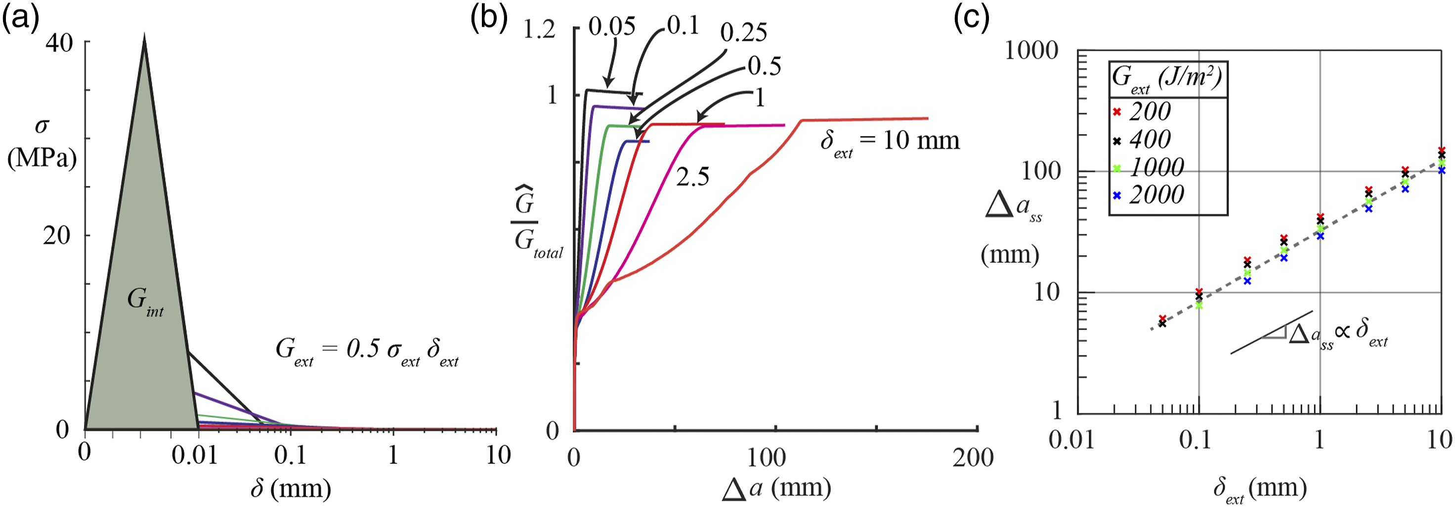$G_{ext}$ . Note: the extrinsic part of the horizontal axis is shown on a log scale. (b) R-curves showing effect of $δ_{e x t}$ for the case with $G_{ext} = 400 J / m^{2}$ and (c) the relationship between the bridging length $δ_{ext}$ and steady-state crack length ${Δa}_{ss}$ .

We note in passing that the input fracture energies in the cohesive law (i.e. the total, $G_{t o t a l}$ ) are not completely recovered in the measured values $\hat{G}$ , i.e. $\hat{G} / G_{t o t a l} < 1$ . This error arises from the ASTM data reduction methods which are replicated here in silico. The data reduction methods consider the bending of the arms of the DCB specimen and beam rotations at the crack tip are accounted for; however, this method does not account for the tractions behind the crack as a result of fibre bridging. A follow-up study will examine this effect in detail in the context of the data reduction methods as described in the ASTM standard³⁰ and their appropriateness in the presence of fibre bridging or other extrinsic mechanisms.

Reproduction of experimentally observed behaviour

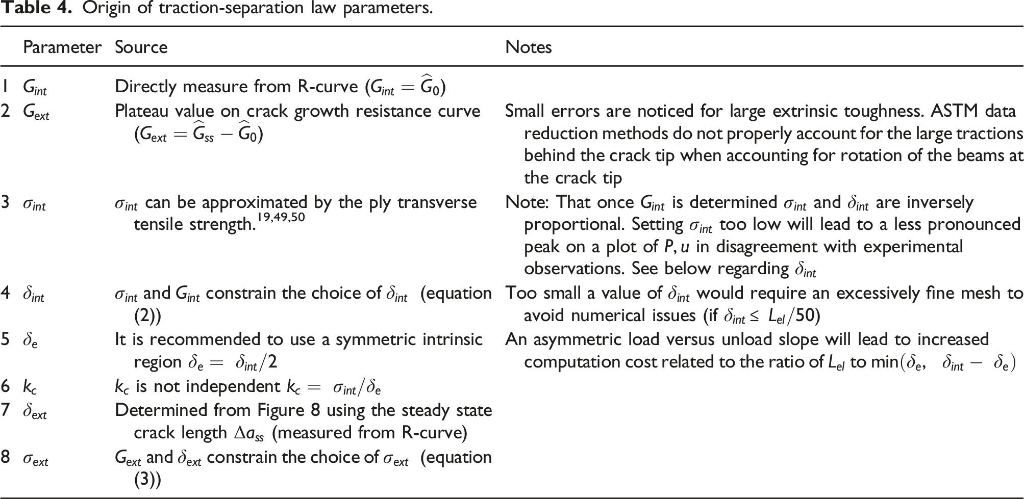
Based on the above results, a strategy for determining traction-separation properties (suitable for use in simulation) from experimental data (such as the example shown in Figure 8(a)) is suggested (Table 4). The quantities needed for Table 4 are also shown in Figure 8(a) and determined from a simplification of the experimental data (i.e. considering only ${\hat{G}}_{0}$ , ${\hat{G}}_{s s}$ , and $Δ a_{s s}$ ). The previously established relationships above ( $Δ a_{s s} \propto E^{1 / 3}$ and $Δ a_{s s} \propto h$ ) are combined with the relationship established in Figure 7(c) ( $Δ a_{s s} \propto δ_{e x t}$ ) to relate $Δ a_{s s}$ to $E, h & δ_{e x t}$ as shown in Figure 8(b).

Figure 8.

(a) Measurement of $G_{i n t}$ , $G_{e x t}$ and $Δ a_{s s}$ from simplification (green) of an R-curve.²² (b) Previously established relationship between ${Δa}_{ss}$ and $E, h & δ_{ext}$ ; used to calculate $δ_{e x t}$ .

Table 4.

Origin of traction-separation law parameters.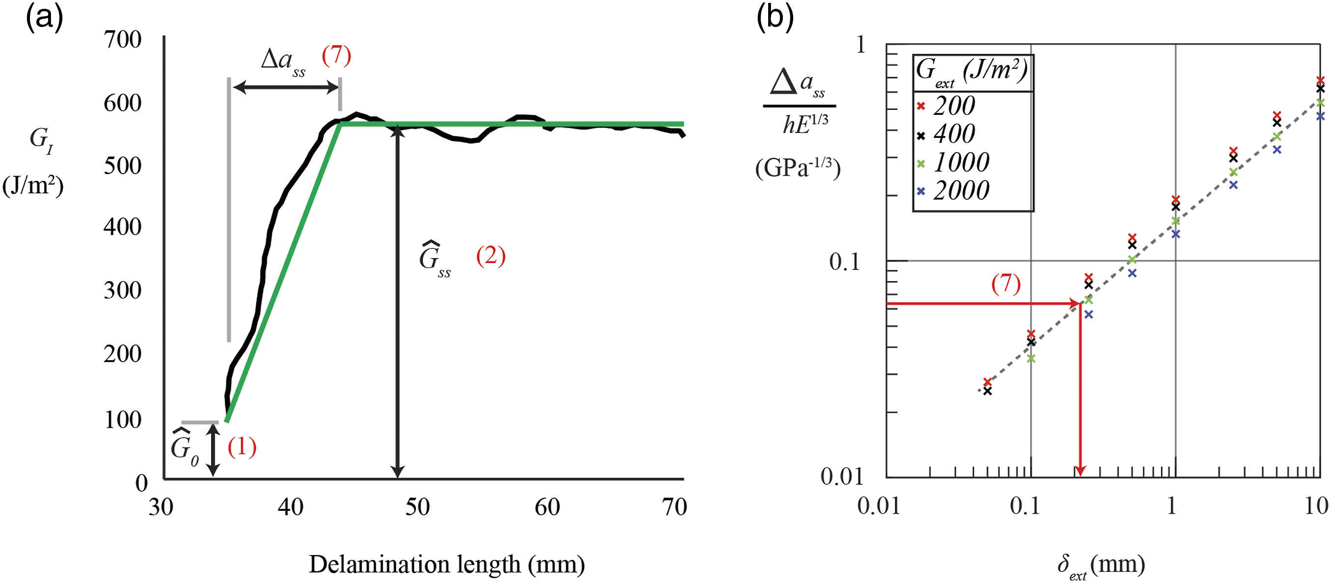

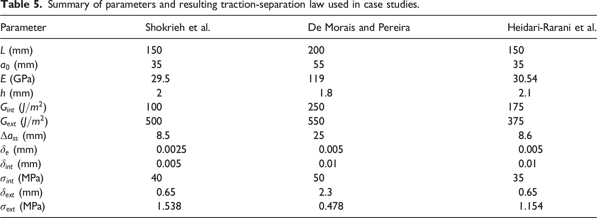
	Parameter	Source	Notes
1	$G_{i n t}$	Directly measure from R-curve ( $G_{i n t} = {\hat{G}}_{0}$ )
2	$G_{e x t}$	Plateau value on crack growth resistance curve ( $G_{e x t} = {\hat{G}}_{s s} - {\hat{G}}_{0}$ )	Small errors are noticed for large extrinsic toughness. ASTM data reduction methods do not properly account for the large tractions behind the crack tip when accounting for rotation of the beams at the crack tip
3	$σ_{i n t}$	$σ_{i n t}$ can be approximated by the ply transverse tensile strength.^19,49,50	Note: That once $G_{i n t}$ is determined $σ_{i n t}$ and $δ_{i n t}$ are inversely proportional. Setting $σ_{i n t}$ too low will lead to a less pronounced peak on a plot of $P, u$ in disagreement with experimental observations. See below regarding $δ_{i n t}$
4	$δ_{i n t}$	$σ_{i n t}$ and $G_{i n t}$ constrain the choice of $δ_{i n t}$ (equation (2))	Too small a value of $δ_{i n t}$ would require an excessively fine mesh to avoid numerical issues (if $δ_{i n t} \leq L_{e l} / 50$ )
5	$δ_{e}$	It is recommended to use a symmetric intrinsic region $δ_{e} = δ_{i n t} / 2$	An asymmetric load versus unload slope will lead to increased computation cost related to the ratio of $L_{e l}$ to $\min (δ_{e}, δ_{i n t} - δ_{e})$
6	$k_{c}$	$k_{c}$ is not independent $k_{c} = σ_{i n t} / δ_{e}$
7	$δ_{e x t}$	Determined from Figure 8 using the steady state crack length $Δ a_{s s}$ (measured from R-curve)
8	$σ_{e x t}$	$G_{e x t}$ and $δ_{e x t}$ constrain the choice of $σ_{e x t}$ (equation (3))

Case studies

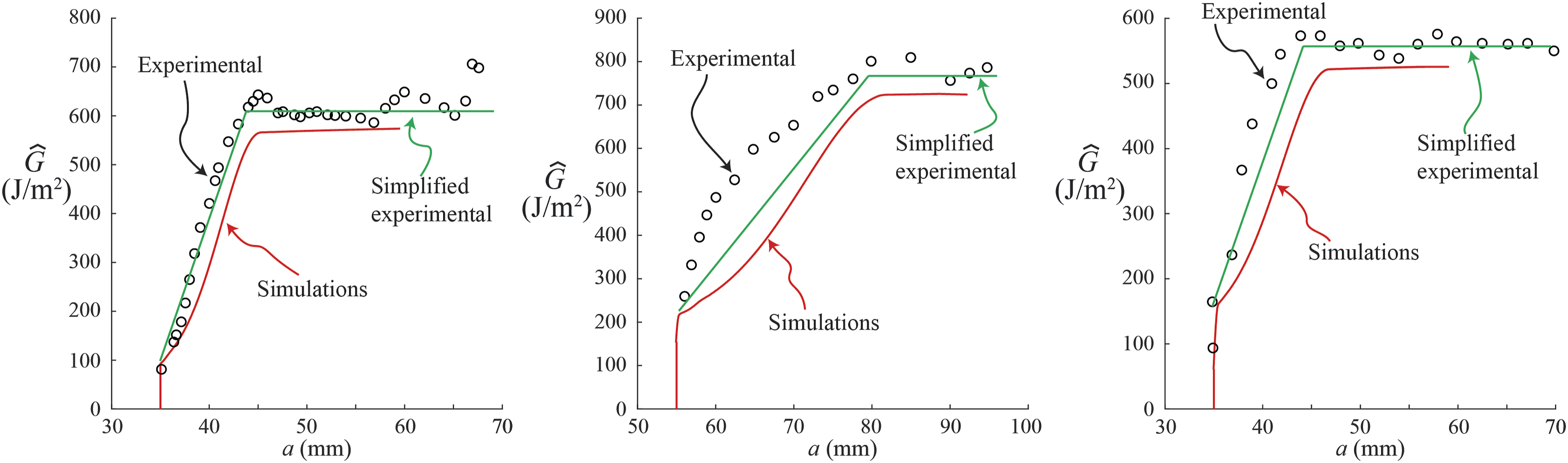
The method outlined above is applied to three experimental data from literature.^22,34,38 Figure 9 below shows the experimental data from these studies (black), the simplified experimental data used as model inputs (green) and resulting simulations (red). The TSL used in these simulations is obtained from the simplification of the experimental data using the procedure in Table 4.

Figure 9.

Case studies comparing experimental data (black symbols) with simulated R-curves (red) using a traction-separation law approximated based on the method described in this study, simplified experimental data shown in green. Left: Shokrieh et al.,³⁴ Middle: De Morais and Pereira,³⁸ Right: Heidari-Rarani et al.²²

The materials used in these case studies encompass a range of material parameters; their properties and resulting traction-separation laws are summarised in Table 5. In all cases, the key features are captured, namely the initial and plateau values of observed tractions, and the crack growth required to get the plateau. The form of the TSL assumed in this work does result in a difference between the slope of the R-curve during the transition region, particularly for the case of the experimental observations of De Morais and Pereira. Capturing the exact shape would require an arbitrarily shaped TSL and is beyond the scope or intent of the present work. Similar to the observations made above regarding the influence of fibre bridging on the ASTM data reduction methods, the plateau value of the measured toughness is below that of the experimental data and the reduced/simplified data (which informed the model inputs).

Table 5.

Summary of parameters and resulting traction-separation law used in case studies.

Parameter	Shokrieh et al.	De Morais and Pereira	Heidari-Rarani et al.
$L$ (mm)	150	200	150
$a_{0}$ (mm)	35	55	35
$E$ (GPa)	29.5	119	30.54
$h$ (mm)	2	1.8	2.1
$G_{i n t}$ ( $J / m^{2}$ )	100	250	175
$G_{e x t}$ ( $J / m^{2}$ )	500	550	375
$Δ a_{s s}$ (mm)	8.5	25	8.6
$δ_{e}$ (mm)	0.0025	0.005	0.005
$δ_{i n t}$ (mm)	0.005	0.01	0.01
$σ_{i n t}$ (MPa)	40	50	35
$δ_{e x t}$ (mm)	0.65	2.3	0.65
$σ_{e x t}$ (MPa)	1.538	0.478	1.154

Concluding remarks

By providing an in-depth exploration of the parameter space associated with a traction-separation law (TSL), the shape of a crack growth resistance curve (R-curve) can be explained in detail. For extrinsic toughening mechanisms such as fibre bridging, the maximum separation at which the bridging tractions act was found to be the key cohesive property to be tuned to capture the main features of an R-curve (i.e. the initial and steady state toughness values and the crack growth required to reach the steady state value). For cohesive behaviour with only intrinsic toughening mechanisms, the cohesive stiffness and maximum traction do not control the behaviour––it is the intrinsic fracture toughness which dictates the behaviour. However, as bridging tractions are substantially less than the maximum intrinsic traction, a trilinear TSL is required to capture bridging behaviour. These observations are used to establish a procedure to robustly identify the input parameters for use in a computational model (i.e. with a traction-separation law).

For cohesive behaviour with extrinsic toughening mechanisms such as fibre bridging, the relationship between the key features of an observed crack growth resistance curve and the input TSL have been robustly explored and key trends are identified. Examination of these trends has shown that the key features on an R-curve (the initial value, the plateau in toughness and the steady-state crack length) can be explained in terms of the interfacial law. The initial value ${\hat{G}}_{0}$ required for crack initiation is the intrinsic fracture toughness $G_{i n t}$ , the plateaued value ${\hat{G}}_{s s}$ is the total fracture energy $G_{t o t a l}$ in the model. The steady-state crack length $Δ a_{s s}$ , required to achieve a plateau in the R-curve, is a function of beam thickness, modulus and fibre bridging length $δ_{e x t}$ (a cohesive property).

The method outlined in this paper is on purely mode I cracks; however, in many scenarios, mixed mode loading leads to delamination of plies. Assuming a simple bilinear law for the mode II fracture behaviour, a minimum of four additional parameters would be added to this study (three mode II TSL parameters and a mode mixity term). Including extrinsic toughening via a trilinear law would increase this to five mode II TSL parameters. Performing a similar exploration of the parameter space for mixed mode loading is feasible; however, reducing the data to a similar robust set of guidelines may not be achievable. An experimental validation of pure mode II delamination using the End Notched Flexure test method⁵² could be used to determine mode II parameters; however, it is not clear on the level of complexity required to accurately capture mixed mode behaviour reproduction of experimental results has shown that this method of determining a TSL is accurate. These results facilitate improved understanding of crack growth resistance through quick interpretation of experimental data. By replicating the experimental procedures in the processing of the simulations (rather than for example numerical calculating the J-integral), our results are directly relevant to the experimental testing and calibration of models. The input parameters for finite element simulations can be quickly determined and employed in analyses of end-use scenarios and applications, e.g. in composite structures such as wing surfaces or turbine blades. Correctly capturing the effect of such toughening mechanisms is critical for prediction of failure via inter-laminate cracking in large scale composite structures.

Nomenclature

a

Crack length

a_{0}

Pre-crack length

Δ a_{s s}

Crack length to achieve steady-state distribution of fibres

b

Beam width

E

Young’s modulus

G_{t o t a l}

Total fracture energy

G_{e x t}

Extrinsic fracture energy

G_{i n t}

Intrinsic fracture energy

\hat{G}

Observed fracture energy

{\hat{G}}_{0}

The initial value of fracture toughness on a resistance curve (R-curve)

{\hat{G}}_{s s}

Plateau value of fracture toughness on a R-curve

h

Beam thickness (one laminate)

L

Beam length

L_{e l}

Length of one side of an element

n

Linear regression fitting parameter for compliance calibration method

P

Load

u

Load-line displacement

δ_{e}

Traction-separation law length for elastic damage

δ_{i n t}

Traction-separation law length for intrinsic behaviour

δ_{e x t}

Traction-separation law length for fibre bridging

δ_{m a x}

Traction-separation law maximum length

σ_{i n t}

Maximum allowable traction

σ_{e x t}

Fibre bridging maximum traction

σ_{y t, 90 °}

Transverse ply tensile strength

Footnotes

Acknowledgements

The authors gratefully acknowledge funding, raw materials, and discussion provided by industry partner Hexcel Composites, Duxford, UK and funding provided by the NUI Galway College of Engineering and Informatics Postgraduate Scholarship. The authors acknowledge computational resources provided by the Irish Centre for High-End Computing (ICHEC).

Declaration of conflicting interests

The author(s) declared no potential conflicts of interest with respect to the research, authorship, and/or publication of this article.

Funding

The author(s) received no financial support for the research, authorship, and/or publication of this article.

ORCID iDs

Bobby Huxford

William Ronan

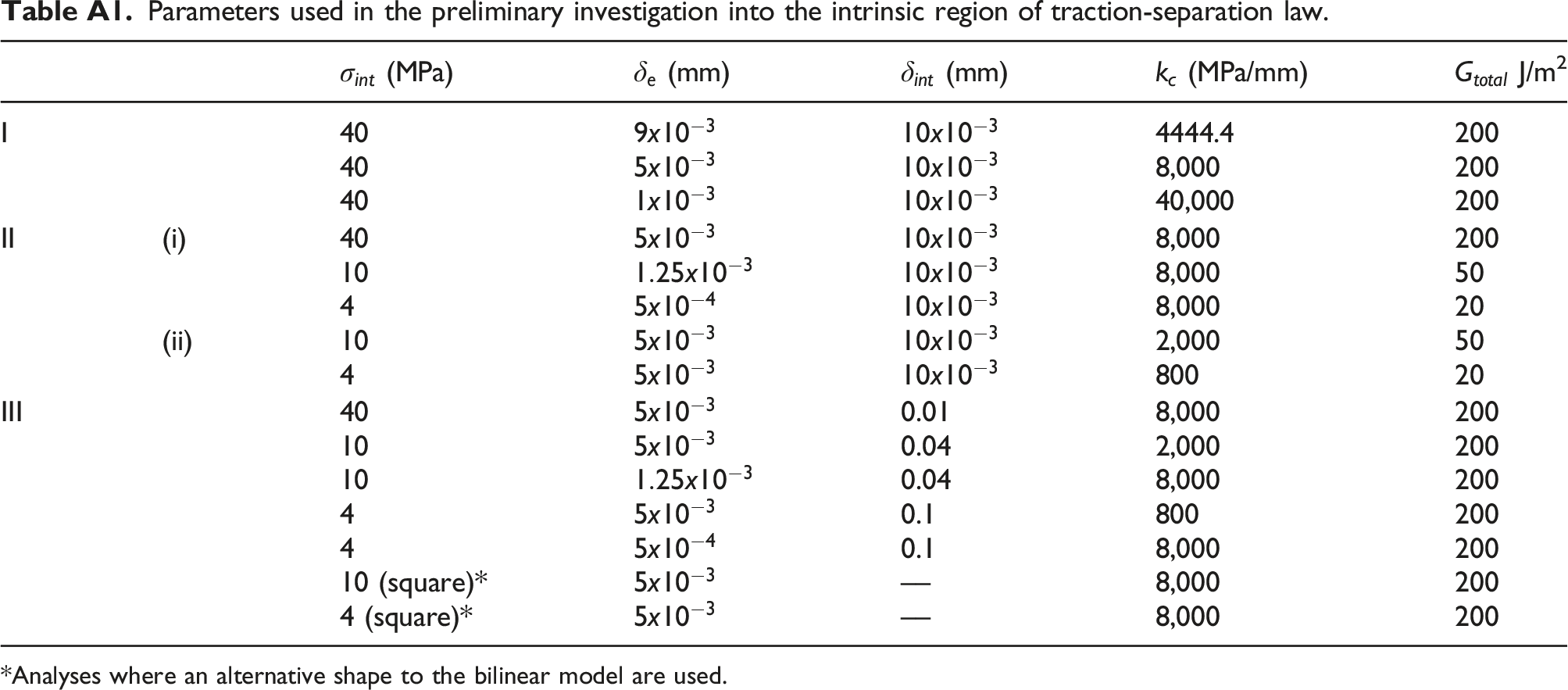
Examining the intrinsic region of the traction-separation law

In the simplest case, with no fibre bridging, the traction-separation curve is completely defined by the stiffness $k_{c}$ , maximum traction $σ_{i n t}$ , and a final separation $δ_{i n t}$ at which the traction returns to zero. This shape of TSL is commonly used in mode II loading as fibre bridging is motivated by mode I opening.⁵¹ Preliminary work in this study involves a systematic variation of the parameter space associated with the intrinsic region of the TSL, i.e. a law without fibre bridging present. The parameter space is explored in three phases: as shown below. Table A1 shows in detail the parameters used and the first column of Figure A1 presents the traction-separation laws input into the simulations in the preliminary work of this investigation.

I. The stiffness $k_{c}$ varies but the traction $σ_{i n t}$ and failure separation $δ_{i n t}$ are fixed.

II. The maximum traction $σ_{i n t}$ is varied. In this case the fracture energy $G_{t o t a l}$ is allowed to change (the failure separation is fixed).

i. The stiffness $k_{c}$ is fixed, therefore the elastic separation $δ_{e}$ is variable.

ii. The elastic separation $δ_{e}$ is held constant; hence $k_{c}$ is variable.

III. The maximum traction $σ_{i n t}$ is varied, for each of the three stiffness values listed above. In this case the fracture energy $G_{t o t a l}$ is kept constant. Different shapes of traction-separation laws are examined including isosceles triangles, scalene triangles, and trapezoids. These laws all have the same fracture energy $G_{t o t a l}$ as calculated by the integral $G_{t o t a l} = \int σ \partial δ$ .

Table A1.

Parameters used in the preliminary investigation into the intrinsic region of traction-separation law.

		$σ_{int}$ (MPa)	$δ_{e}$ (mm)	$δ_{int}$ (mm)	$k_{c}$ (MPa/mm)	$G_{total}$ J/m²
I		40	$9 x 10^{- 3}$	$10 x 10^{- 3}$	4444.4	200
		40	$5 x 10^{- 3}$	$10 x 10^{- 3}$	8,000	200
		40	$1 x 10^{- 3}$	$10 x 10^{- 3}$	40,000	200
II	(i)	40	$5 x 10^{- 3}$	$10 x 10^{- 3}$	8,000	200
		10	$1.25 x 10^{- 3}$	$10 x 10^{- 3}$	8,000	50
		4	$5 x 10^{- 4}$	$10 x 10^{- 3}$	8,000	20
	(ii)	10	$5 x 10^{- 3}$	$10 x 10^{- 3}$	2,000	50
	(ii)	4	$5 x 10^{- 3}$	$10 x 10^{- 3}$	800	20
III		40	$5 x 10^{- 3}$	0.01	8,000	200
		10	$5 x 10^{- 3}$	0.04	2,000	200
		10	$1.25 x 10^{- 3}$	0.04	8,000	200
		4	$5 x 10^{- 3}$	0.1	800	200
		4	$5 x 10^{- 4}$	0.1	8,000	200
		10 (square)*	$5 x 10^{- 3}$	––	8,000	200
		4 (square)*	$5 x 10^{- 3}$	––	8,000	200

*Analyses where an alternative shape to the bilinear model are used.

Figure A1.

Summarised input parameters and results from the intrinsic study, i.e. no fibre bridging present.

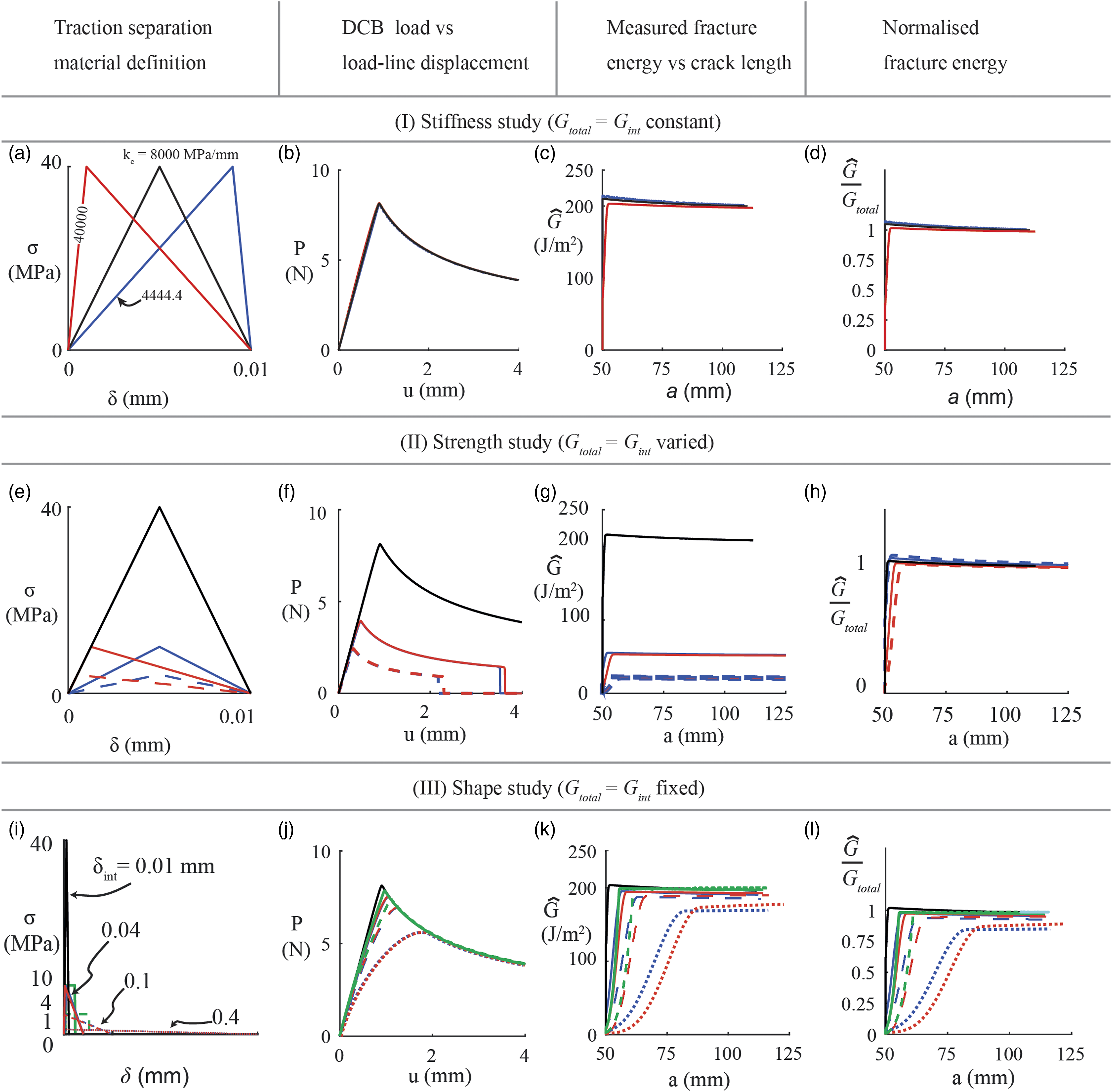
The stiffness study (Figure A1(a)–(d)) shows that the macroscopic behaviour of a DCB (without bridging) is not affected by the value of $k_{c}$ . Regardless of the value of $k_{c}$ , the P-u plot shows the same behaviour; hence the measured toughness $\hat{G}$ does not vary as shown in the R-curves.

In the strength study (Figure A1(e)–(h)), the maximum traction influences the peak value in the P-u plot and the plateau in the R-curve, however once normalised using the total area under the TSL (i.e. the total input fracture energy $G_{t o t a l}$ ), the maximum traction has little effect on the R-curve.

Finally, by varying the shape of the TSL (Figure A1(i)–(l)), similar trends were observed; once normalised, the R-curve was the same. In contrast, the TSL with the very large $δ_{i n t}$ was noticeably different with a gradually increasing toughness. However, this TSL is not representative of material with only intrinsic toughening as $δ_{i n t}$ is unphysically large. Such behaviour is more appropriately examined with a TSL that incorporates bridging as explored in this study.

References

Argon

Cohen

. Toughenability of polymers. Polymer (Guildf) 2003; 44: 6013–6032.

Cepeda-Jiménez

Pozuelo

García-Infanta

, et al. Influence of the alumina thickness at the interfaces on the fracture mechanisms of aluminium multilayer composites. Mater Sci Eng A 2008; 496: 133–142.

Liu

Jia

, et al. Interfacial characterization, control and modification of carbon fiber reinforced polymer composites. Compos Sci Technol 2015; 121: 56–72.

Sills

Thouless

. Cohesive-length scales for damage and toughening mechanisms. Int J Solids Struct 2015; 55: 32–43.

Nairn

. Matrix microcracking. Damage Mechanics of Composite Materials. Elseveir Science, 1994, pp. 1–46.

Sorem

Dodds

Rolfe

. Effects of crack depth on elastic-plastic fracture toughness. Int J Fract 1991; 47: 105–126.

Orowan

. Fracture and strength of solids. Rep Prog Phys 1949; 12: 309–332.

Kovar

Thouless

Halloran

. Crack deflection and propagation in layered silicon nitride/boron nitride ceramics. J Am Ceram Soc 1998; 81: 1004–1012.

Smith

. Crack bifurcation in brittle solids. J Mech Phys Solids 1968; 16: 329–336.

10.

Beachem

Yoder

. Elastic-plastic fracture by homogeneous microvoid coalescence tearing along alternating shear planes. Metall Trans 1973; 4: 1145–1153.

11.

Watanabe

Khera

Vargas

, et al. Fracture toughness comparison of six resin composites. Dent Mater 2008; 24: 418–425.

12.

Compston

Jar

PYB

. Influence of fibre volume fraction on the mode I interlaminar fracture toughness of a glass-fibre/vinyl ester composite. Appl Compos Mater 1999; 6: 353–368.

13.

Cha

Y-H

Kim

K-S

Kim

D-J

. Evaluation on the fracture toughness and strength of fiber reinforced brittle matrix composites. KSME Int J 1998; 12: 370–379.

14.

Meo

Thieulot

. Delamination modelling in a double cantilever beam. Compos Struct 2005; 71: 429–434.

15.

Tonsomboon

Koh

Oyen

. Time-dependent fracture toughness of cornea. J Mech Behav Biomed Mater 2014; 34: 116–123.

16.

Parmigiani

Thouless

. The roles of toughness and cohesive strength on crack deflection at interfaces. J Mech Phys Solids 2006; 54: 266–287.

17.

Thouless

Waas

, et al. Use of mode-I cohesive-zone models to describe the fracture of an adhesively-bonded polymer-matrix composite. Compos Sci Technol 2005; 65: 281–293.

18.

Thouless

Waas

, et al. Use of a cohesive-zone model to analyze the fracture of a fiber-reinforced polymer-matrix composite. Compos Sci Technol 2005; 65: 537–549.

19.

De Morais

. A new fibre bridging based analysis of the Double Cantilever Beam (DCB) test. Compos Part A Appl Sci Manuf 2011; 42: 1361–1368.

20.

De Morais

. Double cantilever beam testing of multidirectional laminates. Compos Part A Appl Sci Manuf 2003; 34: 1135–1142.

21.

Manshadi

Farmand-Ashtiani

Botsis

, et al. An iterative analytical/experimental study of bridging in delamination of the double cantilever beam specimen. Compos Part A 2014; 61: 43–50.

22.

Heidari-Rarani

Shokrieh

Camanho

. Finite element modelling of mode I delamination growth in laminated DCB specimens with R-curve effects. Compos Part B Eng 2013; 45: 897–903.

23.

Gokgol

Basdogan

Canadinc

. Estimation of fracture toughness of liver tissue: experiments and validation. Med Eng Phys 2012; 34: 882–891.

24.

Comley

Fleck

. A micromechanical model for the Young’s modulus of adipose tissue. Int J Solids Struct 2010; 47: 2982–2990.

25.

Shahmansouri

Cartier

Mongrain

. Characterization of the toughness and elastic properties of fresh and cryopreserved arteries. J Biomech 2015; 48: 2205–2209.

26.

Ammann

Niemz

. Fibre and adhesive bridging at glue joints in European beech wood. Wood Res 2014; 59: 303–312.

27.

Vasic

Smith

. Bridging crack model for fracture of spruce. Eng Fract Mech 2002; 69: 745–760.

28.

Liu

Huang

Geng

, et al. Multiscale hierarchical structure and laminated strengthening and toughening mechanisms. In: Osheku CA (ed). Lamination - Theory and Application [Internet]. London: IntechOpen, 2017 [cited 2022 Jul 02]. https://www.intechopen.com/chapters/56537

29.

Gutkin

Laffan

Pinho

, et al. Modelling the R-curve effect and its specimen-dependence. Int J Solids Struct 2011; 48: 1767–1777.

30.

ASTM . Standard Test Method for Mode I Interlaminar Fracture Toughness of Unidirectional Fiber-Reinforced Polymer Matrix Composites, 2013, pp. 1–13.

31.

Davidson

Waas

. Non-smooth mode I fracture of fibre-reinforced composites: an experimental, numerical and analytical study. Philos Trans R Soc A 2012; 370: 1942–1965.

32.

Rikards

Buchholz

Wang

, et al. Investigation of mixed mode I/II interlaminar fracture toughness of laminated composites by using a CTS type specimen. Eng Fract Mech 1998; 61: 325–342.

33.

Schiffer

Tagarielli

. Predictions of the interlaminar tensile failure of a carbon/epoxy composite laminate. Compos Struct 2015; 133: 997–1008.

34.

Shokrieh

Salamat-Talab

Heidari-Rarani

. Effect of initial crack length on the measured bridging law of unidirectional E-glass/epoxy double cantilever beam specimens. Mater Des 2014; 55: 605–611.

35.

Elices

Guinea

Omez

, et al. The cohesive zone model: advantages, limitations and challenges. Eng Fract Mech 2002; 69: 137–163.

36.

Jacobsen

Sørensen

. Mode I intra-laminar crack growth in composites––modelling of R-curves from measured bridging laws. Compos Part A Appl Sci Manuf 2001; 32: 1–11.

37.

Blackman

BRK

Hadavinia

Kinloch

, et al. The calculation of adhesive fracture energies in mode I: revisiting the tapered double cantilever beam (TDCB) test. Eng Fract Mech 2003; 70: 233–248.

38.

De Morais

Pereira

. Application of the effective crack method to mode I and mode II interlaminar fracture of carbon/epoxy unidirectional laminates. Compos Part A 2007; 38: 785–794.

39.

Rice

. A path independent integral and the approximate analysis of strain concentration by notches and cracks. J Appl Mech 1968; 35: 379–386.

40.

Sørensen

Jacobsen

. Determination of cohesive laws by the J integral approach. Eng Fract Mech 2003; 70: 1841–1858.

41.

Ward

. A novel testing for post-peak tensile behavior of cementitious composites. Fract Toughness Fract Energy 1989; 1989: 183–195.

42.

Brenet

Conchin

Fantozzi

, et al. Direct measurement of crack-bridging tractions: A new approach to the fracture behaviour of ceramic/ceramic composites. Compos Sci Technol 1996; 56: 817–823.

43.

Zhu

Liechti

Ravi-Chandar

. Direct extraction of rate-dependent traction–separation laws for polyurea/steel interfaces. Int J Solids Struct 2009; 46: 31–51.

44.

Sørensen

Jacobsen

. Large-scale bridging in composites: R-curves and bridging laws. Compos Part A Appl Sci Manuf 1998; 29: 1443–1451.

45.

Holmes

Liu

Sørensen

, et al. Experimental approach for mixed-mode fatigue delamination crack growth with large-scale bridging in polymer composites. J Compos Mater 2014; 48: 3111–3128.

46.

Airoldi

Dávila

. Identification of material parameters for modelling delamination in the presence of fibre bridging. Compos Struct 2012; 94: 3240–3249.

47.

Dávila

Rose

Camanho

. A procedure for superposing linear cohesive laws to represent multiple damage mechanisms in the fracture of composites. Int J Fract 2009; 158: 211–223.

48.

Systemes

. Abaqus user manual. 2010.

49.

De Morais

De Moura

MFSF

. Assessment of initiation criteria used in interlaminar fracture tests of composites. Eng Fract Mech 2005; 72: 2615–2627.

50.

Hodgkinson

. Mechanical testing of advanced fibre composites. Cambridge, England: Woodhead Publishing, 2000.

51.

Borotto

. Bridging effects on Mixed Mode delamination : experiments and numerical simulation. PhD Thesis. École Polytechnique Fédérale de Lausanne, 2016, p. 67.

52.

ASTM . Standardization of the end-notched flexure test for mode II interlaminar fracture toughness determination of unidirectional laminated composites. ASTM 2015; 43: 6.

Fibre bridging: Continuum modelling of extrinsic toughening in double cantilever beam tests

Abstract

Keywords

Introduction

Intrinsic and extrinsic toughening

Experimental fracture tests with fibre bridging

Data analysis

Determining cohesive properties

Modelling approach

Finite element model

Parameter variation details

Results

The ratio of extrinsic to intrinsic toughness ( G ext : G int )

Effect of fracture test properties

Bridging length and steady-state crack length

Reproduction of experimentally observed behaviour

Case studies

Concluding remarks

Nomenclature

Footnotes

Acknowledgements

Declaration of conflicting interests

Funding

ORCID iDs

Examining the intrinsic region of the traction-separation law

References

The ratio of extrinsic to intrinsic toughness $(G_{ext} : G_{int})$