A resistor network model for analysis of current and temperature distribution in carbon fibre reinforced polymers during induction heating

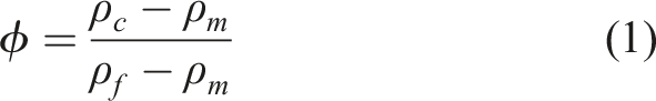
Abstract

The interest in carbon fibre reinforced polymers (CFRP) is growing due to their high strength and stiffness compared to their weight, in industries such as automotive and aerospace. This creates a high demand for more effective production methods. Volumetric induction heating of the electrically conductive carbon fibres enable unmatched heat rates and can be used both during manufacturing and joining of parts, but also means technical challenges in terms of uniform temperature distribution. Understanding and prediction of the heating pattern is therefore an important step towards an industrial solution. This article presents a model for simulation of the current and temperature distribution in CFRP during induction heating in which the CFRP is modelled as a network of discrete resistors where the local currents are determined by Kirchhoff’s circuit laws and the temperature distribution is computed by the finite difference method. The model is a complement to traditional three-dimensional finite element simulations and allows for a better understanding of the current paths, and thereby the heating pattern, on a tow size level. Thermographic recordings during induction heating experiments validates the model.

Introduction

Carbon fibre reinforced polymers have high strength to weight ratio which make them interesting within many industries, for example automotive and aerospace, and an enabler for reduction of emissions and energy consumption. The growing interest results in an increasing need for proper and efficient heating methods during manufacturing of the composite, but also for joining of CFRP parts, or for reparation purpose.

Carbon fibres are electrically conductive which makes it possible to heat them by induction, as observed by Miller et al. ¹ and Fink et al. ² Induction heating can be used for welding of thermoplastic CFRP as investigated by Grouve et al. ³ and Rudolf et al. ⁴ Becker et al. ⁵ investigates how the thread count (parallel tows per length unit in a woven fabric) affects the induction heating of CFRP based on thermoplastic matrix. It can also be used for post curing of thermoset parts as investigated by Bettelli et al., ⁶ or for achieving the desired temperature during the entire curing thermoset curing cycle.

One important factor in the development of the technology for induction heating of CFRP is proper modelling tools. For modelling of induction heating in CFRP a common approach is to use the finite element method, for example used by Senghor et al., ⁷ Bui et al., ⁸ Grouve et al., ³ Fu et al., ⁹ Riccio et al., ¹⁰ Tzeng et al. ¹¹ and Lundström et al. ¹² In such models CFRP are often represented as anisotropic homogeneous domains using macroscopic material properties since it would be unmanageable to simulate the induction heating process on microscopic level. One of the most crucial parameters during induction heating of CFRP is the electrical conductivity and its direction dependency. One example of work on this topic is the model developed by Yu et al. ¹³ for predicting the macroscopic electrical conductivity in unidirectional CFRP where the influence from micromechanical properties such as waviness are analysed using an resistor network model. Also Wasselynck et al.^14–16 have developed models for determination of electrical conductivity in CFRP, to be used for finite element simulations of induction heating.

However, computations using three-dimensional finite element models tend to become very heavy due to the vast number of elements required to consider the field gradients (magnetic field and current density field) in three dimensions. Instead the CFRP could be modelled as a network of discrete resistors, on tow size level, without considering the microscopic current density distribution. This is a reasonable approach due to the rapid temperature equalization through the thickness of layers, described by Lundström et al., ¹² making it unnecessary and costly to simulate gradients on microscopic level. Consequently, the resistor network approach could significantly reduce the number of unknowns in comparison to three dimensional finite element models, like the model presented by Fu et al. ⁹ where the mesh size is significantly smaller than the width of a tow. Especially in the case with woven CFRP a resistor network representation would be very intuitive. An example of previous work on the topic is the resistor network model for prediction of heat generation pattern proposed by Kim et al.,^17,18 however without computation of temperature.

This article presents a new approach for computing the induced currents, heating power and temperature distribution in woven CFRP on tow size level, when using an axisymmetric coil. A stepwise procedure is proposed, beginning with solving the electromagnetic problem using an axisymmetric finite element model where the CFRP is represented with an equivalent electrical conductivity.^19–21 From the electromagnetic solution the effective electric field distribution is extracted. Woven CFRP is modelled as a network of discrete resistors where the effective voltage acting over the resistor elements can easily be determined from the electric field distribution from a 2D-axisymmetric FEM model. Due to the in-plane circulating currents, each ply can be modelled as an individual resistor network. The currents in the resistor network are determined by solving a linear equation system based on Kirchhoff’s circuit laws, reducing the need for solving Maxwell’s differential equations in a three-dimensional geometry (woven CFRP and the surrounding air domain). It is also proposed how the simulated geometry can be significantly reduced by exploiting observed symmetries, for the case with a circular coil and a bidirectional woven fabric CFRP. The temperature field is computed using the finite difference method to solve the heat equation and then compared with thermographic measurements during induction heating. Each resistor element is represented with a volume element with uniform temperature which is reasonable due to the rapid through thickness heat equalization in CFRP, shown by Lundström et al. ¹² The resistor network approach reduces the number of unknowns significantly compared to a FEM model where the mesh size needs to be adapted to the gradients; higher gradients requires finer mesh.

Materials

Two CFRP plates with different fibre volume fraction were used to validate the model. The plates were manufactured using vacuum assisted resin transfer moulding and the thickness and fibre volume fraction of the plates are presented in Table 1. The plates have a side length 170 mm and each fabric ply have 59 parallel fibre tows in each direction. Figure 1 shows one of the manufactured CFRP plates and microscopy images of the fibre structures. The average fibre volume fraction ϕ is calculated according to equation ¹ where ρ _c is the density of the CFRP plate, ρ _m is the density of the matrix material and ρ _f is the fibre density. Properties of fibre fabric and epoxy matrix are specified in Table 2. The plates are the same as used in the study by Lundström et al., ²² in which they are denoted Plate 1 (4 plies) and Plate 5 (8 plies).

$$\varphi =\frac{{\rho }_c-{\rho }_m}{{\rho }_f-{\rho }_m}$$

(1)

Table 1.

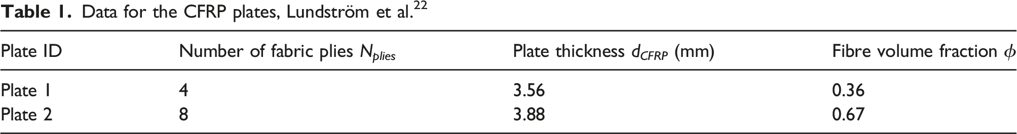
Data for the CFRP plates, Lundström et al. ²²

Plate ID	Number of fabric plies N plies	Plate thickness d CFRP (mm)	Fibre volume fraction ϕ
Plate 1	4	3.56	0.36
Plate 2	8	3.88	0.67

Figure 1.

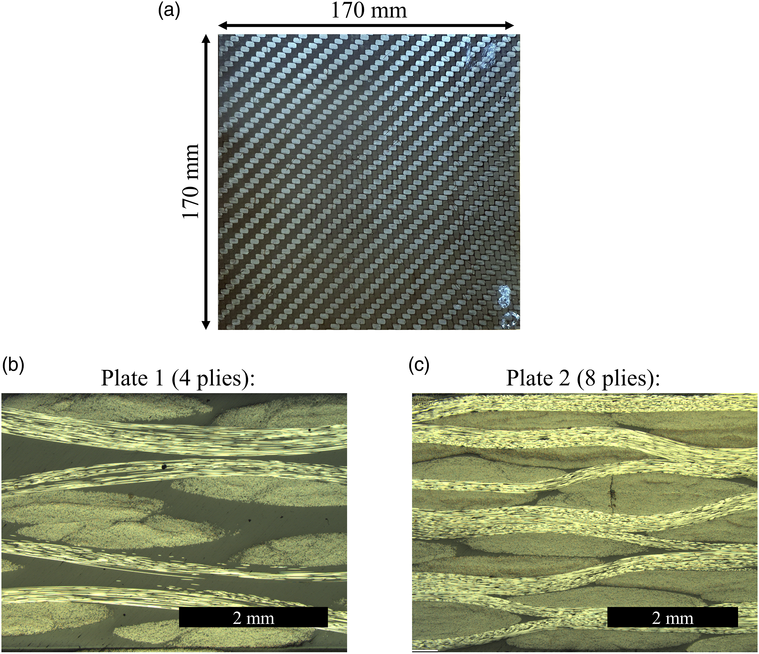
(a) An image of plate two and its outer dimensions. (b) A microscopy image of the through thickness fibre structure for plate 1. (c) A microscopy image of the through thickness fibre structure for plate 2. The microscopy images in (b) and (c) are reprinted from Lundström et al. ²²

Table 2.

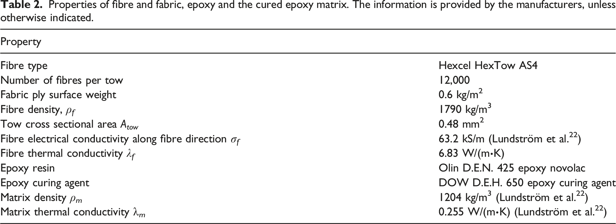
Properties of fibre and fabric, epoxy and the cured epoxy matrix. The information is provided by the manufacturers, unless otherwise indicated.

Property
Fibre type	Hexcel HexTow AS4
Number of fibres per tow	12,000
Fabric ply surface weight	0.6 kg/m2
Fibre density, ρ f	1790 kg/m3
Tow cross sectional area A tow	0.48 mm2
Fibre electrical conductivity along fibre direction σ f	63.2 kS/m (Lundström et al.22)
Fibre thermal conductivity λ f	6.83 W/(m∙K)
Epoxy resin	Olin D.E.N. 425 epoxy novolac
Epoxy curing agent	DOW D.E.H. 650 epoxy curing agent
Matrix density ρ m	1204 kg/m3 (Lundström et al. 22 )
Matrix thermal conductivity λ m	0.255 W/(m∙K) (Lundström et al. 22 )

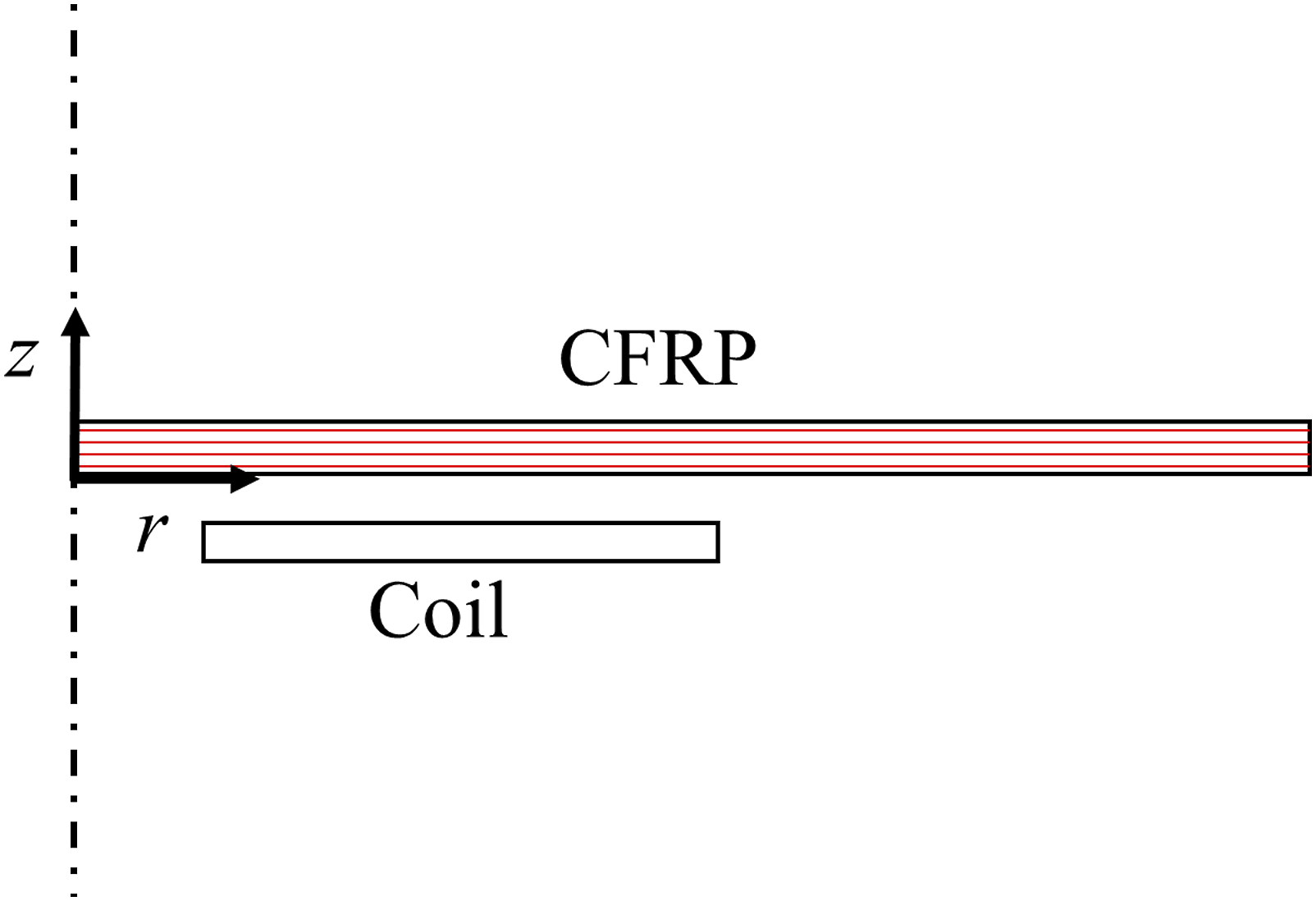
Experimental setup

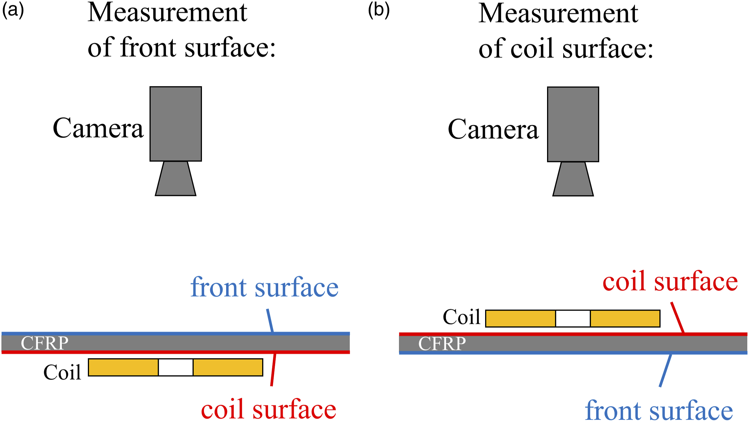
To validate the proposed model, thermographic measurements were performed during induction heating of the CFRP-plates, using the thermographic camera FLIR T540. This will give information of the temperature distribution, but also indirect information of the current and heating power distribution. The coil current was generated using the frequency inverter INV-15kW-1 MHz, with a maximum power of 15 kW, manufactured by Corebon AB. Figure 2 shows the experimental setup for the thermographic measurements of the CFRP plates during induction heating. The same coil and setup was used by Lundström et al.^12,20,22 The coil is placed in a coil holder to fix the distance between the coil and the CFRP plate; 3.8 mm. The coil has 14 turns, made from a litz wire with 500 individually insulated strands with a diameter of 0.1 mm. The coil has the inner diameter 20 mm, the outer diameter 101 mm, and the thickness 3 mm. The plates were painted with a matt black colour to get a surface with known emissivity; with the observed value ϵ = 0.93. The coil current was measured using the Rogowski coil PEM CWT. The induction heating experiments were performed with a 60 kHz sinusoidal coil current. In this article the two surfaces of a CFRP plate are denoted “coil surface” and “front surface. The “coil surface” is the CFRP surface closest to the induction coil and the “front surface” is the CFRP surface on the opposite side of the coil. When recording the front surface the induction coil is placed on the opposite side and therefor the front surface can be recorded during the whole induction heating duration, as illustrated in Figure 3. Recording of the “coil surface” cannot be performed during induction heating since the coil obscures the view for the camera. The coil surface is recorded by placing the coil above the CFRP plate, as illustrated in Figure 3, and after finished induction heating the coil is removed so that the surface can be recorded by the thermographic camera.

Figure 2.

Experimental setup used for thermographic measurements. (a) Shows the thermographic camera recording the “front surface” of the CFRP plate. It also shows the current measurement probe and the capacitor used to achieve electrical resonance. (b) Shows the induction coil placed in the coil holder. (c) Shows the induction coil placed above the CFRP plate for thermographic measurement of the surface closest to the coil, denoted “coil surface” in this study. Reprinted from Lundström et al. ²⁰

Figure 3.

This figure describe with schematic illustrations the placement of coil and CFRP plate in relation to the thermographic camera when recording the front surface or the coil surface. (a) Measurement of the front surface. (b) Measurement of the coil surface. In the latter case (b) the CFRP plate is first inductively heated and then the coil is removed to record the surface.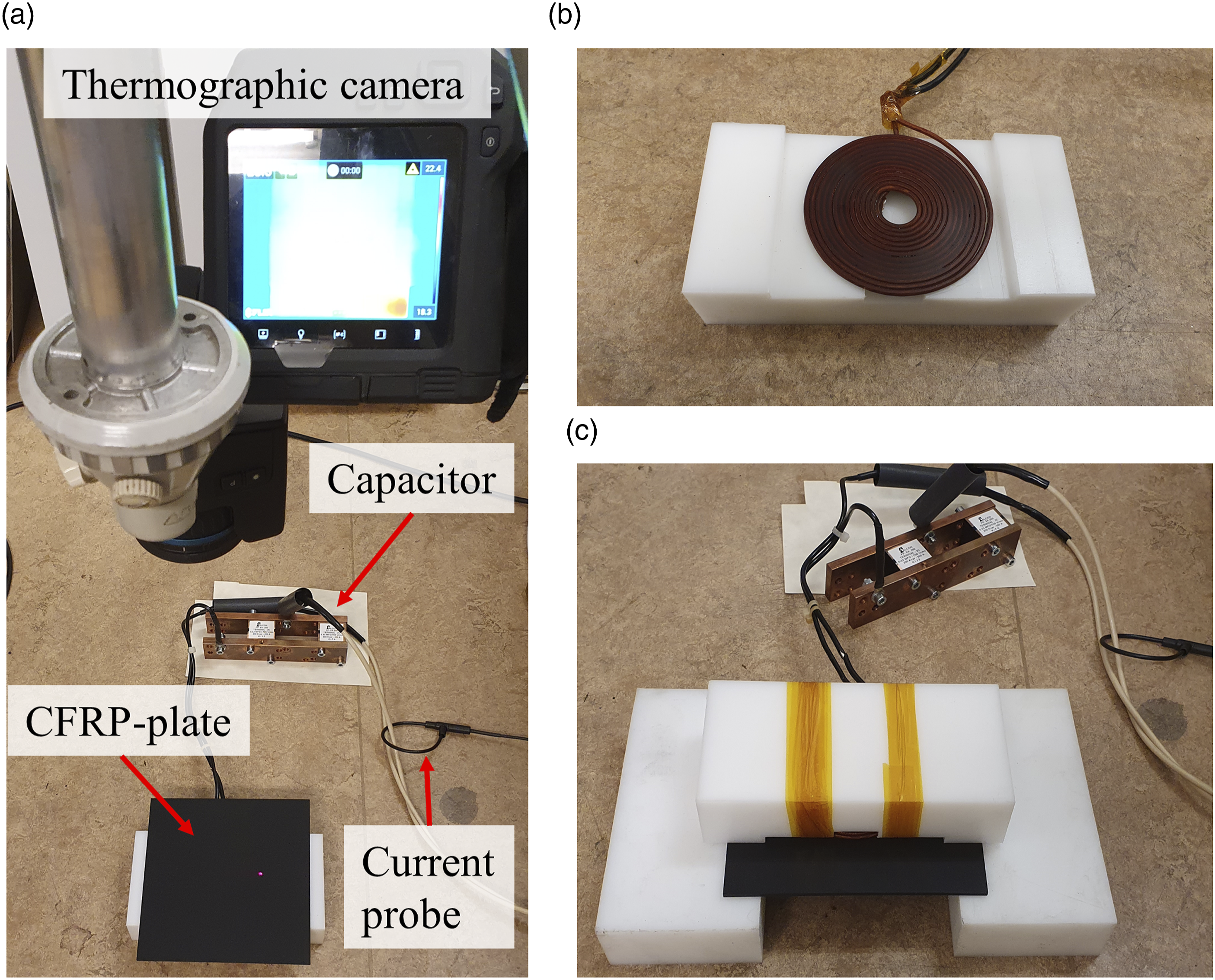

Resistor network model

Current and voltage equations

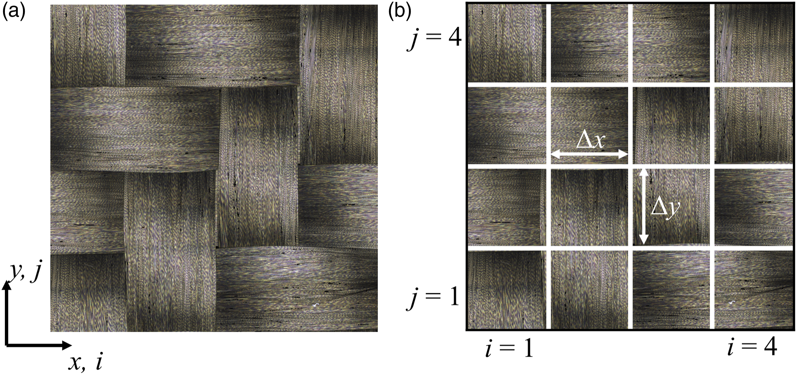
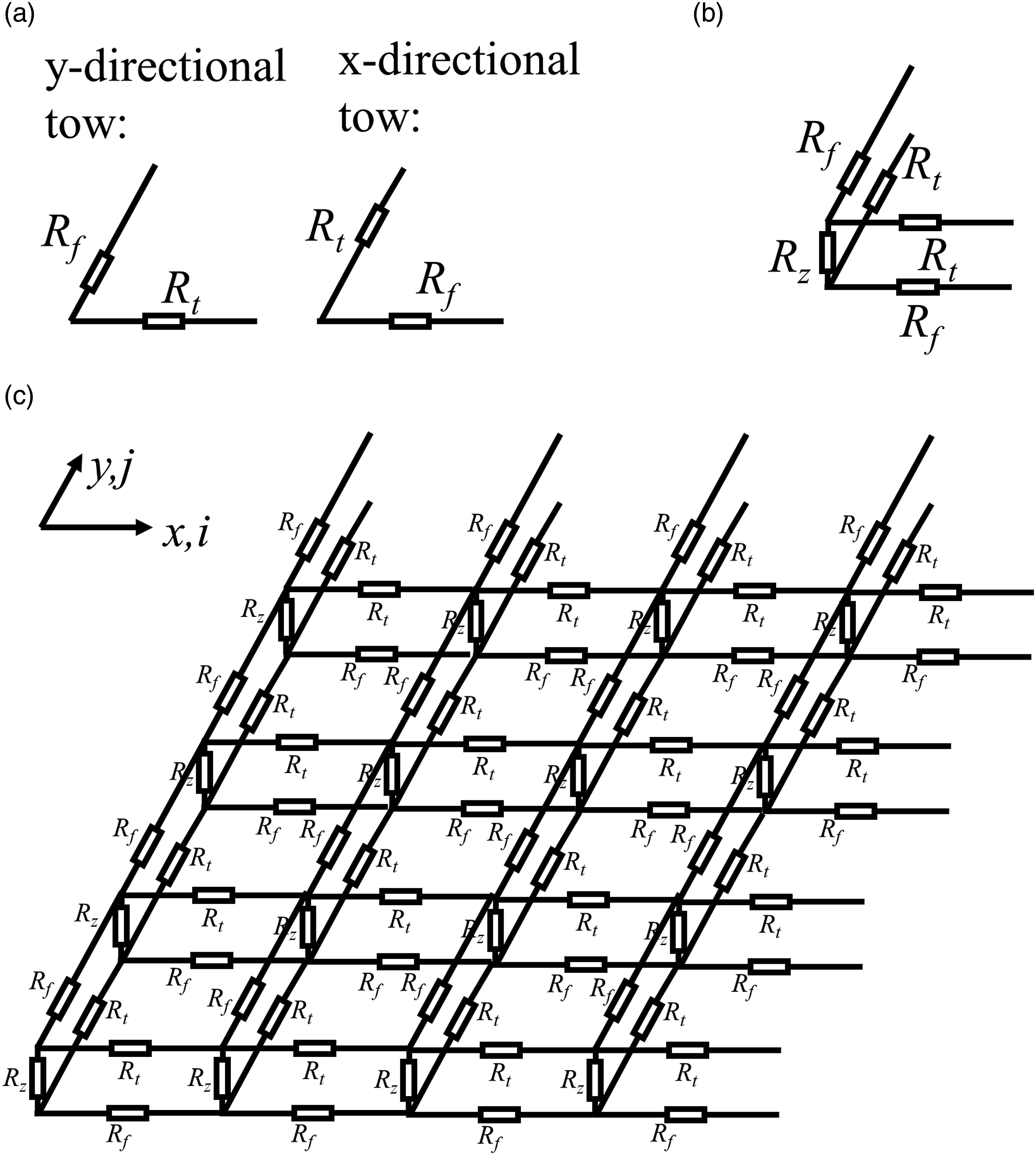
The resistor network model represents one ply of woven fabric. Figure 4 shows how a twill woven carbon fibre fabric is discretized into 4 × 4 elements. Each element has the side lengths Δx and Δy according to equation (2) where s _CFRP is the side length of the plate (s _CFRP = 170 mm) and N _tows is the number of parallel tows in each direction (N _tows = 59 in both x direction and y direction). Figure 5 shows how each discrete element in Figure 4 is represented by a discrete resistor. Each element consists of two perpendicular tow elements represented by a resistance along the fibre direction R _f and a resistance transverse to the fibre direction in the plane R _t as shown in Figure 5(a). Since the elements are square R _f have the same value in x and y direction. This also applies for R _t . The resistor networks for the x-directional and y-directional tows are connected through the resistor R _z , as shown in Figure 5(b). Figure 5(c) shows the whole resulting network representing the 4 × 4 element fabric ply in Figure 4. However, as shown by shown by Lundström et al. ²² it is reasonable to set the electrical conductivity transverse the fibre direction in the plane to zero when inducing circulating currents in-plane, due to the significantly higher electrical conductivity along the fibre direction. This reasoning is also supported by Mizukami and Watanabe. 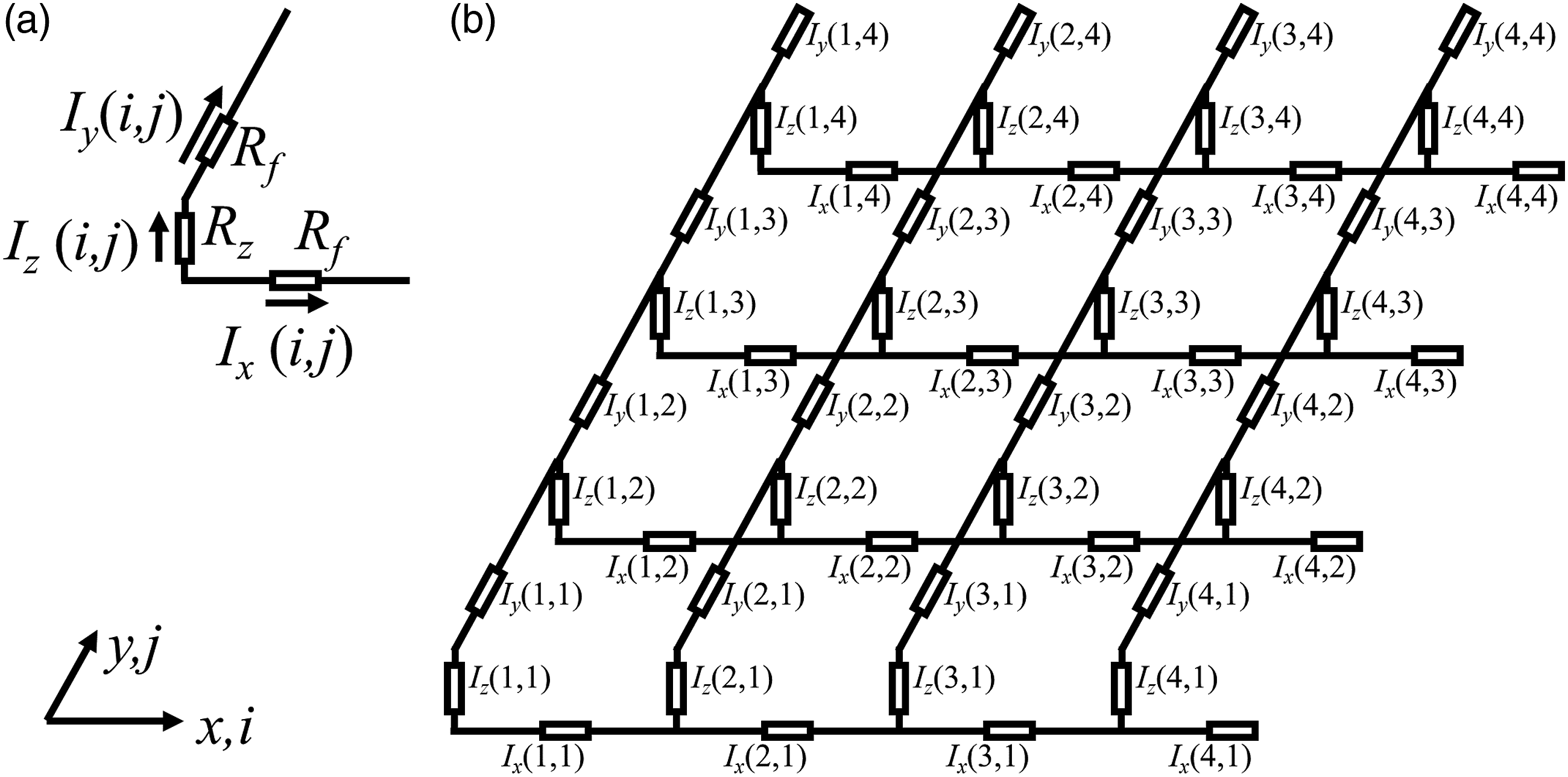²³ Therefore by disregarding R _t the resistor network representation shown in Figure 5 can be simplified according to Figure 6 where each element is represented with three discrete resistors: R _f in x and y direction and R _z in z direction. Each element is assigned with the currents I _x (i,j), I _y (i,j) and I _z (i,j). The symbol m represent the number of elements in the x-direction and n represent the number of elements in the y-direction, illustrated in Figure 4. As observed by Fink et al. ² the electric coupling between crossing fibres may also be due to capacitive coupling and the heating may also be due to dielectric losses. However, as observed by Becker at al. ²⁴ heating due to dielectric losses is negligible compared to the resistive losses. At the relatively low frequency used in this article, 60 kHz, a purely resistive representation have been proved to be a good approximation, Lundström et al.^12,22

$$\mathrm{\Delta }x=\mathrm{\Delta }y=\frac{s_{CFRP}}{N_{tows}}$$

(2)

Figure 4.

This figure illustrates how a woven fabric is discretized to be represented by resistors. (a) Twill woven fabric. (b) Shows how the twill woven fabric is divided into discrete square elements. Each element consists of two perpendicular fibre tows. The variable i denotes the element number in x direction and j denotes the element number in y direction. The photography of the twill fabric is adapted from Lundström et al. ¹⁹

Figure 5.

This figure shows how the discrete elements in Figure 4 are represented by discrete resistors. (a) Shows how x-directional tows and y-directional tows are represented with discrete resistors, one along the fibre direction R _f , and one transverse the fibre direction R _t in the fabric plane. (b) Shows how the x directional, and y directional tows are electrically connected via the R _z resistors. (c) Shows how the piece of woven in Figure 4 is represented with the resistor network.

Figure 6.

(a) One ply element is represented with three resistors when the transverse resistors R _t disregarded. (b) The resulting resistor network, with the current components to be determined, after simplification of the network in Figure 5(c).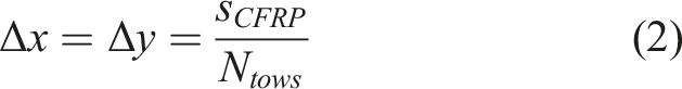

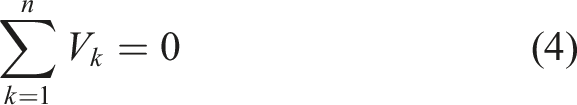
The resistor network currents are determined using Kirchhoff’s circuit laws for current and voltage. Kirchhoff’s current law states that the sum of currents flowing into a node equals zero, expressed in equation (3) where n represents the total number of currents in the network, and I _k is the k:th current flowing into the node. Incoming and outgoing currents from the node have opposite signs. Kirchhoff’s voltage law states that the sum of voltages in a closed loop equals zero, expressed in equation (4) where n represents the total number of voltages in the network and V _k is the k:th voltage in the loop. Figure 7 shows how I _x , I _y and I _z are connected and from this the two governing current equations are derived; one represents the relationship between I _x and I _z , equation (5), and one represents the relationship between I _y and I _z , equation (6). Figure 8 shows how the voltage equation (7) is derived. The arrows in the figures indicate the positive directions. 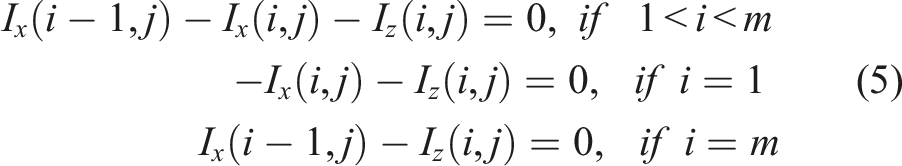The variables V _x and V _y represent the induced voltages in the x and y directions. It is described later in the article how the induced voltages are determined. When the coil is parallel with the CFRP plate no voltage will be induced in the z-direction.

$${\displaystyle \sum }_{k=1}^n{I}_k=0$$

(3)

$${\displaystyle \sum }_{k=1}^n{V}_k=0$$

(4)

$$I_x\left(i-1,j\right)-I_x\left(i,j\right)-I_z\left(i,j\right)=0, if 1<i<m\hspace{0.17em}-I_x\left(i,j\right)-I_z\left(i,j\right)=0, if i=1\hspace{0.17em}\hspace{0.17em}{I}_x\left(i-1,j\right)-I_z\left(i,j\right)=0, if i=m$$

(5)

$$I_y\left(i,j-1\right)-I_y\left(i,j\right)+I_z\left(i,j\right)=0, if 1<j<n\hspace{0.17em}-I_y\left(i,j\right)+I_z\left(i,j\right)=0, if j=1I_y\left(i,j-1\right)+I_z\left(i,j\right)=0, if j=n$$

(6)

$$-I_x\left(i,j\right)\cdot R_x+I_x\left(i,j+1\right)\cdot R_x+I_y\left(i,j\right)\cdot R_y-I_y\left(i+1,j\right)\cdot R_y+I_z\left(i,j\right)\cdot R_z-I_z\left(i,j+1\right)\cdot R_z+I_z\left(i+1,j+1\right)\cdot R_z-I_z\left(i+1,j\right)\cdot R_z=-V_x\left(i,j\right)+V_x\left(i,j+1\right)+V_y\left(i,j\right)-V_y\left(i+1,j\right), if i\le m-1 \& j\le n-1$$

(7)

Figure 7.

The figure illustrates how the currents in x direction are connected with the currents in y direction through the current in z-direction. From this the current equations (5) and (6) are derived.

Figure 8.

The voltages are summed in the direction of the circulating arrow to derive the voltage equation (7). The left hand side of the equation contains the voltage drops over the resistors due to the currents flowing through them and the right hand side contains the induced voltages.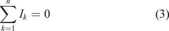

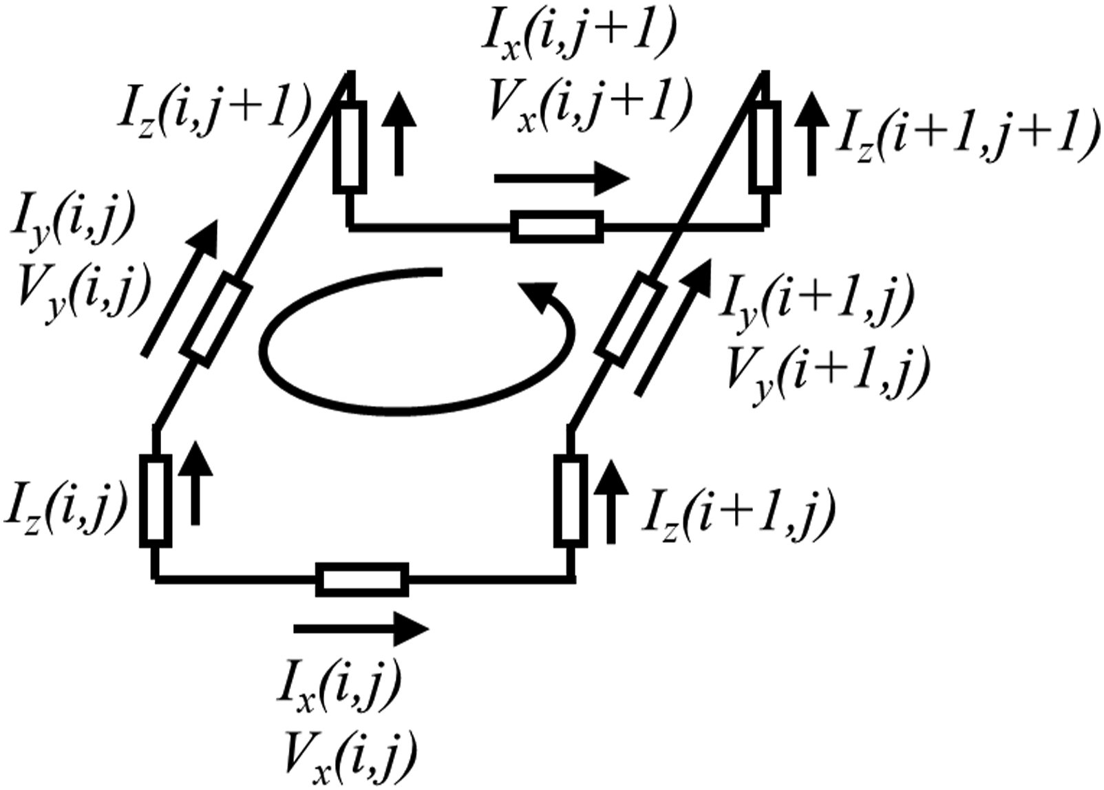
Since every element contains three current components the potential number of unknown current components are the number of elements times three. However, as can be seen in Figure 6 the resistor network contains loose ends in the x and y directions in which the current will be zero, given by the conditions in equations (5) and (6). These equations also implies that I _z (m,n) can be determined according to equation (8) and thus reduced from the equation system. Therefore, the total number of unknown current components will be according to equation (9). Each element is associated with two current equations (5) and (6), and all elements except the ones on the outer edge (i = m and j = n) are associated with a voltage equation. Since the current I _z (m,n) is reduced from the equation system, also the two current equations associated with this can be reduced. Thus, the total number of available equations is determined according to equation (10) which equals the number of unknowns, and therefore the equation system can be solved.

$$I_z\left(m,n\right)=I_x\left(m-1,n\right)$$

(8)

$$N_{unknowns}=\left(m-1\right)n+\left(n-1\right)m+mn-1=3mn-m-n-1$$

(9)

$$N_{equations}=2mn+\left(m-1\right)\left(n-1\right)-2=3mn-m-n-1$$

(10)

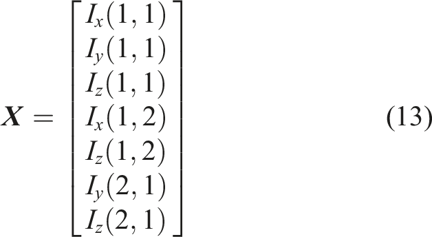
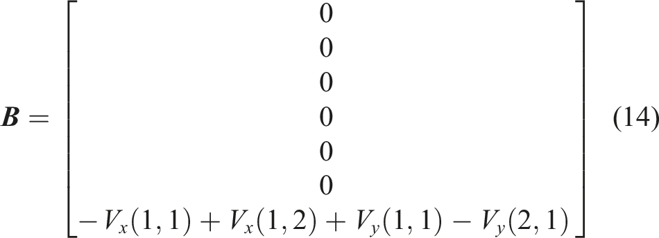
The equations (5)–(7) are arranged in a linear equation system on the form shown in equation (11) and solved using a linear solver in Matlab. Each unknown current component is assigned a row in the X array and each equation is assigned a row in the A matrix. The B array is assigned the values of the right-hand side in the equations.

$$\mathit{AX=B}$$

(11)

Equations (12)–(14) show an example of the resulting equation system for the case with only 2 × 2 elements, i.e. only one possible current loop and thus only one voltage equation.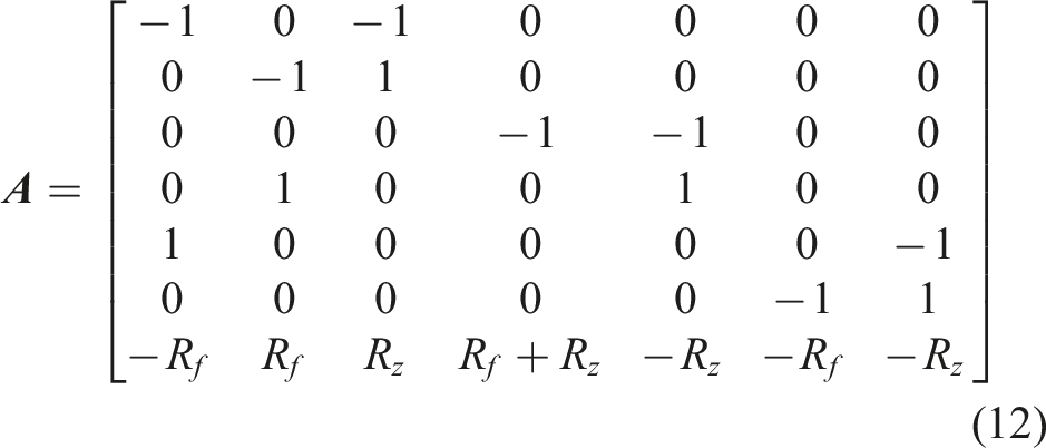

$$\mathit{A}=\left[\begin{array}{ccccccc}-1& 0& -1& 0& 0& 0& 0\\ 0& -1& 1& 0& 0& 0& 0\\ 0& 0& 0& -1& -1& 0& 0\\ 0& 1& 0& 0& 1& 0& 0\\ 1& 0& 0& 0& 0& 0& -1\\ 0& 0& 0& 0& 0& -1& 1\\ -R_f& R_f& R_z& R_f+R_z& -R_z& -R_f& -R_z\end{array}\right]$$

(12)

$$\mathit{X}=\left[\begin{array}{c}{I}_x\left(\mathrm{1,1}\right)\\ I_y\left(\mathrm{1,1}\right)\\ I_z\left(\mathrm{1,1}\right)\\ I_x\left(\mathrm{1,2}\right)\\ I_z\left(\mathrm{1,2}\right)\\ I_y\left(\mathrm{2,1}\right)\\ I_z\left(\mathrm{2,1}\right)\end{array}\right]$$

(13)

$$\mathit{B}=\left[\begin{array}{c}0\\ 0\\ 0\\ 0\\ 0\\ 0\\ -V_x\left(\mathrm{1,1}\right)+V_x\left(\mathrm{1,2}\right)+V_y\left(\mathrm{1,1}\right)-V_y\left(\mathrm{2,1}\right)\end{array}\right]$$

(14)

The heating power generated in each resistor of an element is computed according to equations (15)–(17)

$$P_x\left(i,j\right)=R_f{I}_x^2\left(i,j\right)$$

(15)

$$P_y\left(i,j\right)=R_f{I}_y^2\left(i,j\right)$$

(16)

$$P_z\left(i,j\right)=R_z{I}_z^2\left(i,j\right)$$

(17)

Characterization of resistance and induced voltage

The element resistance R _f is calculated according to equation (18), with the resulting value 0.095 Ω. The value of the electrical conductivity of fibre σ _f and the cross-sectional area of a tow A _tow are presented in Table 2.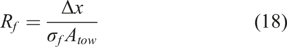

$$R_f=\frac{\mathrm{\Delta }x}{{\sigma }_f{A}_{tow}}$$

(18)

As shown by Lundström et al. ²⁰ an axisymmetric finite element model can be used to approximate the temperature distribution in a bidirectional woven CFRP plate during induction heating with a parallel circular coil. Therefore, such a model could be used to compute the induced electric field, and thus obtain an approximation of the through thickness distribution of the induced power, without the need for solving maxwells equations in the 3D resistor network, thus significantly reducing the number of nodes. Equation (19) gives the relationship between the number of nodes in the 2D finite element model compared to the corresponding 3D model, given that the mesh is uniformly distributed. The geometry is a circular cylinder. The variables have the following meanings: r – radius, h – height, p – number of nodes per length unit. The relationship between number of nodes and computational time is not linear and therefore the benefit of reducing the number of nodes is obvious.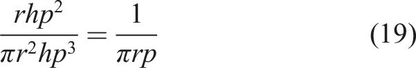

$$\frac{rh{p}^2}{\pi r^{2}h{p}^3}=\frac{1}{\pi rp}$$

(19)

Figure 9 shows the geometry of the electromagnetic axisymmetric finite element model, presented by Lundström et al., ²⁰ implemented using the software COMSOL Multiphysics. A 60 kHz sinusoidal current was applied to the coil (like in the experiments). The model is used to extract the effective value (root mean square) of the induced electric field. Since the CFRP plates are square, their geometry cannot be directly transferred to an axisymmetric representation. However, the axisymmetric representation is considered a reasonable simplification for cases when the coil is smaller than the plate and the induction heating does not result in noticeable edge heating effects, Lundström et al. 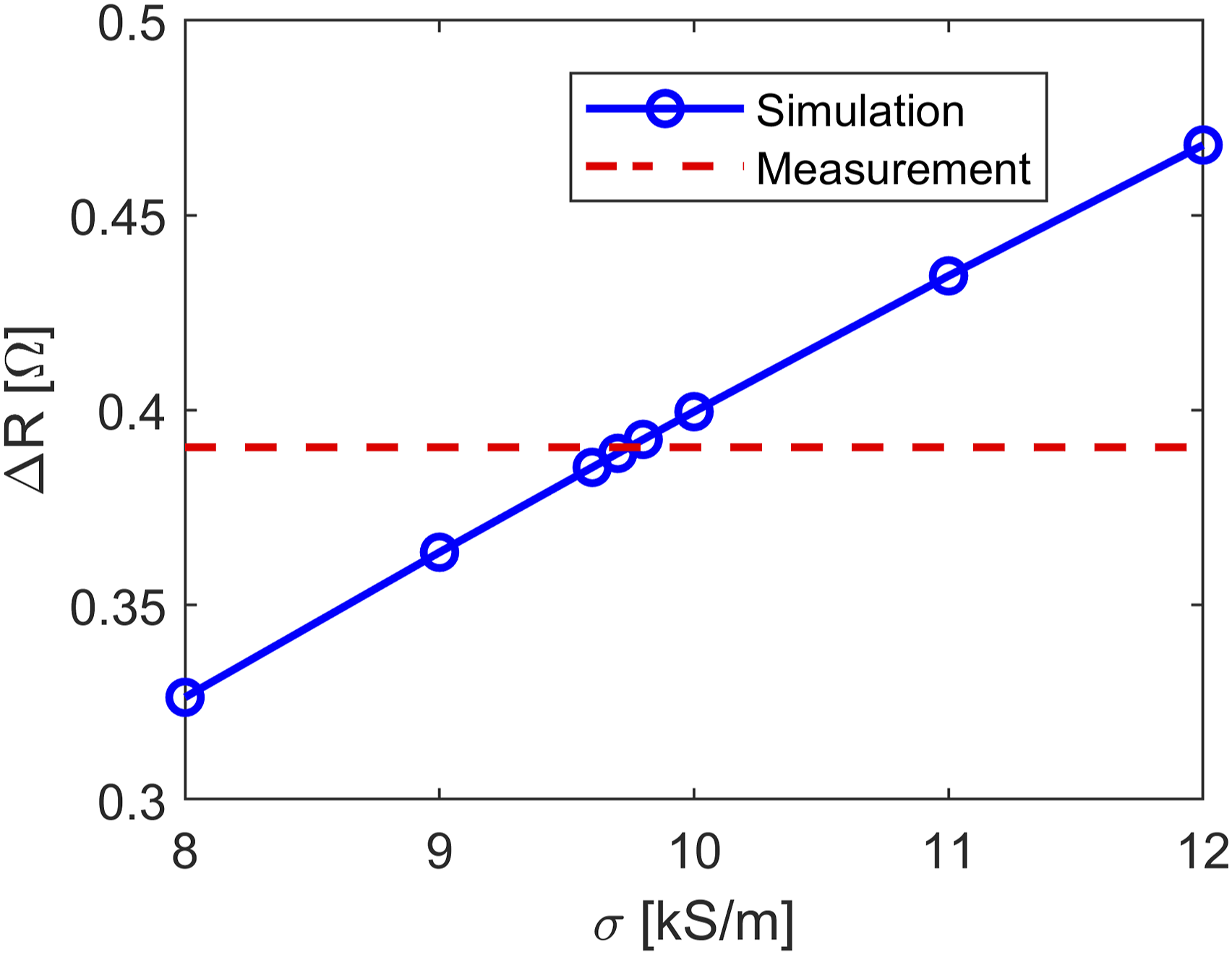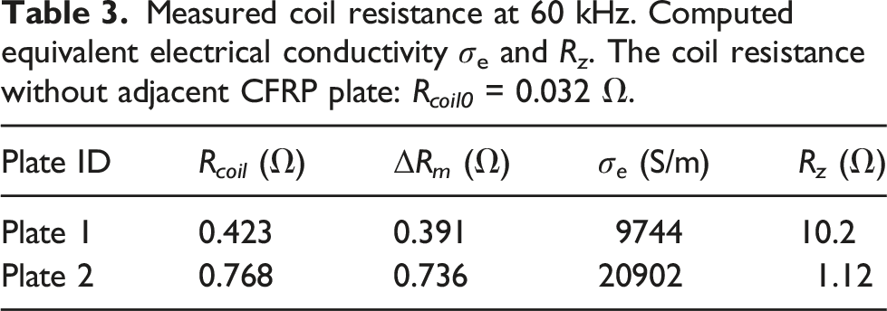²⁰ Therefore, an equivalent radius of the plate is calculated according to equation (22). The CFRP-domain is assigned the equivalent electrical conductivity according to Lundström et al.^19,20 by comparing the measured coil resistance with the simulated coil resistance. The setup is the same as presented in Figure 2. The coil resistance is measured with and without adjacent CFRP plate at the frequency used during the induction heating measurements, 60 kHz. Thus, the coil resistance increase caused by the CFRP can be determined according to equation (20), where R _coil is the coil resistance with adjacent CFRP plate and R _coil0 is the coil resistance without adjacent CFRP plate. Thus, ΔR will be proportional to the energy induced in the CFRP plate. Since the induced power depends on the electrical conductivity of the CFRP plate, the equivalent electrical conductivity σ _e is determined such that the simulated coil resistance increase ΔR _s equals the measured coil resistance increase ΔR _m according to equation (21), illustrated in Figure 10. The values of R _coil , ΔR _m and σ _e are presented in Table 3. The significant difference in R _z between the two plates is due to the fact that the contact resistance between fibres decrease exponentially with increasing fibre volume, analogous with the exponential increase in transverse electrical conductivity as observed by Lundström et al.^12,22

$$\mathrm{\Delta }R=R_{coil}-R_{coil0}$$

(20)

$$\mathrm{\Delta }{R}_s\left(\sigma \right)=\mathrm{\Delta }{R}_m$$

(21)

Figure 9.

Geometry of the axisymmetric finite element model, based on the coil setup, Figure 2. The coil has the inner radius 10.1 mm, the outer radius 50.5 mm, and the thickness 3 mm. The distance between CFRP plate and coil is 3.8 mm. Details about the model, for example boundary conditions, are described by Lundström et al. ²⁰

Figure 10.

Simulated ΔR as function of the electrical conductivity in the CFRP domain of plate 1. The red dashed line represents the measured value to show the point where the simulation and measurement equals each other.

Table 3.

Measured coil resistance at 60 kHz. Computed equivalent electrical conductivity σ_e and R _z . The coil resistance without adjacent CFRP plate: R _coil0 = 0.032 Ω.

Plate ID	R coil (Ω)	ΔR m (Ω)	σ e (S/m)	R z (Ω)
Plate 1	0.423	0.391	9744	10.2
Plate 2	0.768	0.736	20902	1.12

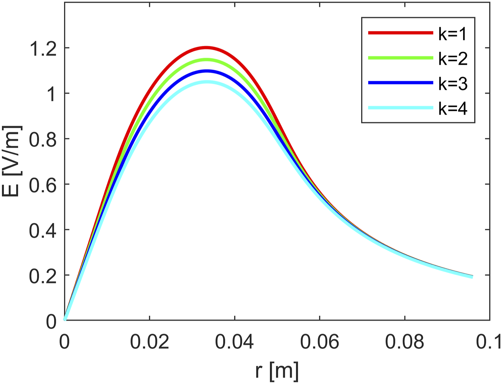
The induced electric field in the k:th ply is approximated by the electrical field at the distance z(k) from the coil-surface of the plate according to equation (23). The lines at which the electric field is extracted are illustrated in Figure 9. Figure 11 shows the electric fields extracted for plate 1 (4 plies) for the effective coil current I _coil = 1 A. Since the coil is parallel with the CFRP plate the electric field is only acting normal to the axisymmetric plane and thus only give rise to voltages over the x and y directional resistors. The radial position r of the element at position (i,j), in relation to the centre position of the coil (i _c ,j _c ), is calculated according to equation (24) where Δz is according to equation (35). The electric field components E _x and E _y acting over each element are calculated according to equations (25) and (26)^. The effective value (root mean square) of the electric field is used. These equations create an electric field, rotating in the positive direction. The induced voltages over each resistor V _x (i,j,k) and V _y (i,j,k) are then calculated according to equations (27) and (28).

$$r_{CFRP}=\sqrt{\frac{s_{CFRP}^2}{\pi }}$$

(22)

$$z\left(k\right)=2\mathrm{\Delta }z\left(k-1\right)+\mathrm{\Delta }z$$

(23)

$$r\left(i,j\right)=\sqrt{{\left(\mathrm{\Delta }x\cdot \left(i-i_c\right)\right)}^2+{\left(\mathrm{\Delta }y\cdot \left(j-j_c\right)\right)}^2}$$

(24)

$$E_x\left(i,j,k\right)=-E\left(r\left(i,j\right),z\left(k\right)\right)\cdot \frac{\mathrm{\Delta }y\cdot \left(j-j_c\right)}{r\left(i,j\right)}$$

(25)

$$E_y\left(i,j,k\right)=E\left(r\left(i,j\right),z\left(k\right)\right)\cdot \frac{\mathrm{\Delta }x\cdot \left(i-i_c\right)}{r\left(i,j\right)}$$

(26)

$$V_x\left(i,j,k\right)=E_x\left(i,j,k\right)\cdot \mathrm{\Delta }x$$

(27)

$$V_y\left(i,j,k\right)=E_y\left(i,j,k\right)\cdot \mathrm{\Delta }y$$

(28)

Figure 11.

The electric field E (r,z) as function of the radius r plotted for the four plies in plate 1, for the effective coil current 1 A.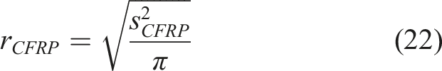

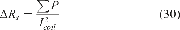
The contact resistance between crossing tows R _z was determined using an inductive method equivalent to the method for computing the through thickness electrical conductivity in cross ply CFRP, by Mizukami and Watanabe ²³ and Lundström et al.^12,22 The measured coil resistance increase ΔR _m is proportional to the induced resistive losses in the CFRP plate. The simulated coil resistance increase ΔR _s is computed according to equation (30), where ΣP is the total induced power in the plate, according to equation (29) at the effective coil current I _coil . The coil resistance was measured with the same distance between coil and plate as used during the thermographic measurements; 3.8 mm. The resistance R _z is computed such that equation (31) is satisfied. The simulated value of ΔR _coil is presented in Figure 12 together with the measured value. The determined values of R _z are presented in Table 3.

$${{\displaystyle \sum }}^{\text{}}P={\displaystyle \sum }_{i=1}^m{\displaystyle \sum }_{j=1}^n{\displaystyle \sum }_{k=1}^{N_{plies}}{P}_x\left(i,j,k\right)+P_y\left(i,j,k\right)+P_z\left(i,j,k\right)$$

(29)

$$\mathrm{\Delta }{R}_s=\frac{{{\displaystyle \sum }}^{\text{}}P}{I_{coil}^2}$$

(30)

$$\mathrm{\Delta }{R}_s\left(R_z\right)=\mathrm{\Delta }{R}_m$$

(31)

Figure 12.

Simulated ΔR as function of the resistance R _z in the CFRP domain of plate 1. The dashed line represent the measured value to show the point where the simulation and measurement equals each other.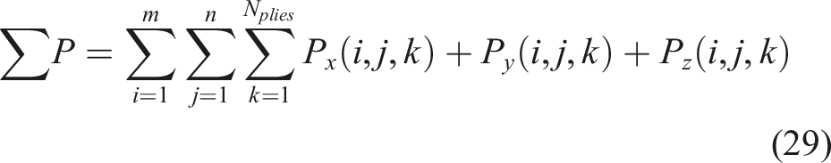

Symmetry conditions and simplifications

For the case with a bidirectional fibre layup and a circular coil parallel with the CFRP plate the symmetry can be exploited, and the geometry can be reduced to one fourth, as observed by Lundström et al., ¹² thus reducing the number of unknowns to a fourth. As can be observed in the temperature distributions recorded by Lundström et al.^20,22 the induction heating of woven fabric CFRP results in four quadrants with the same temperature distribution, shifted 90° in relation to each other. This means that it would be reasonable to do the approximation that current distribution is the same in the interface between the quadrants, as illustrated by Figure 13 and equation (32). The variable k represents the fabric ply number. The ply closest to the coil have ply number k = 1.

$${\displaystyle \sum }_{i=i_c}^m{I}_y\left(i,j_c,k\right)=-{\displaystyle \sum }_{j=j_c}^n{I}_x\left(i_c,j,k\right)=-{\displaystyle \sum }_{i=1}^{i_c}{I}_y\left(i,j_c,k\right)={\displaystyle \sum }_{j=1}^{j_c}{I}_x\left(i_c,j,k\right)$$

(32)

Figure 13.

The figure illustrates the symmetry lines (dashed white lines) when the coil is placed centred parallel with the CFRP plate, marking the interfaces between the quadrants. Each fabric ply consist of 59 parallel tows in each direction (x and y) which is indicated in the figure. The summation of the currents crossing the symmetry lines between the quadrants are indicated and their relationship are expressed in equation (32).

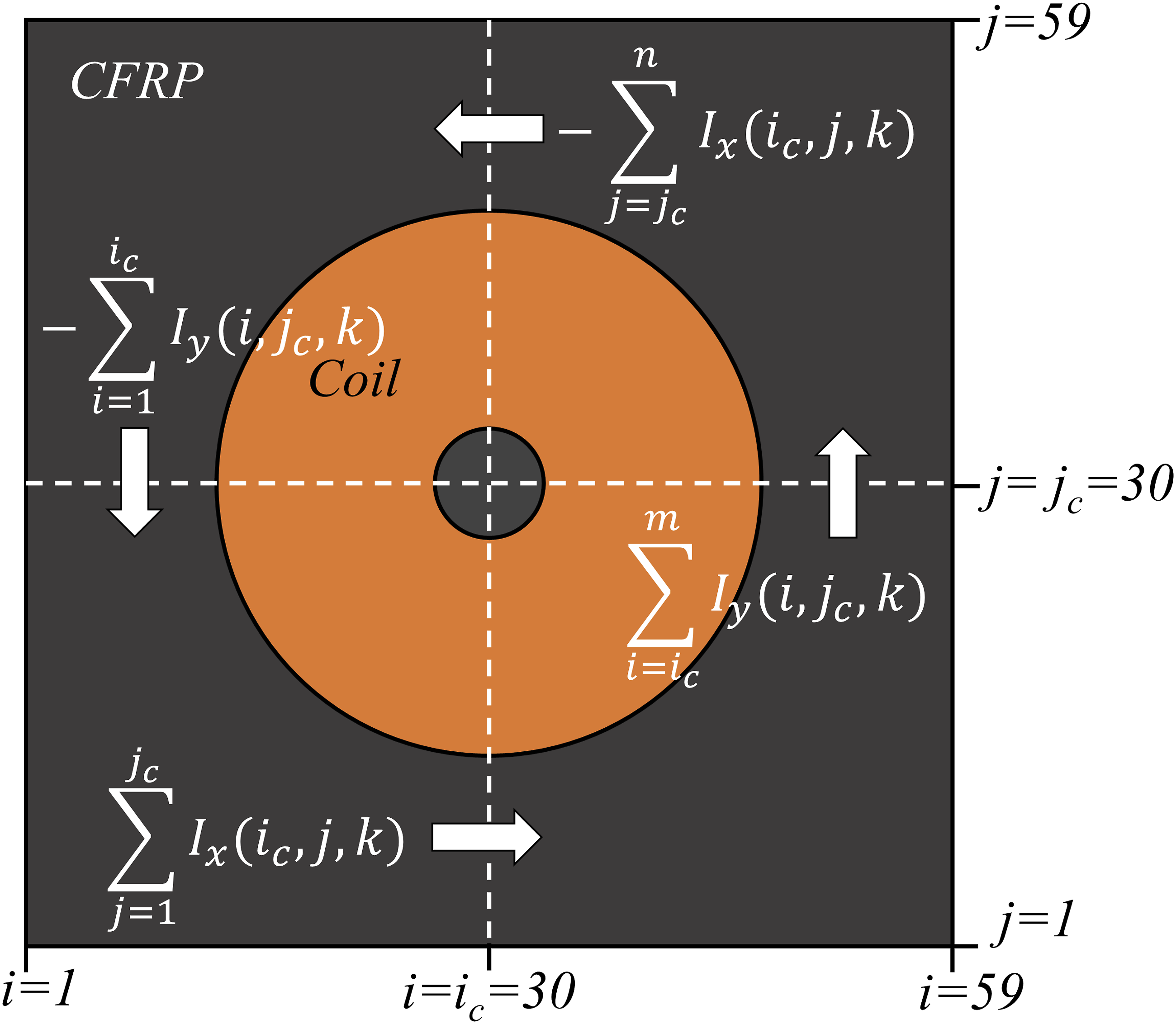
It is also necessary to consider the electrical contact between the fabrics, but a discretization of the contact between adjacent plies is difficult since a well-defined pattern of contact points does not exist. However, according to the following reasoning some simplifications can be made for modelling of the case with bidirectional woven fabric and a parallel circular coil: The quadrant symmetry, equation (32), implies that the current is conserved within each quadrant of a ply when the current flows from x-directional to y-directional tows. Figure 14 shows a lumped element model of the current flow in the first quadrant (upper right in Figure 13) for the case with four parallel fabric plies. According to equation (32) it can be concluded that, within each quadrant the current flow between plies will be zero, as expressed in equation (33). Since the induced voltages are extracted from the axisymmetric FEM model the current distribution in each ply can therefore be solved independently from each other, reducing the computational cost since the computational complexity of solving a linear equation system (matrix inversion) is not linearly dependent on the number of unknowns. The mentioned simplifications are only valid for this specific case with a circular coil and bidirectional fabric. For all other cases, new assessments must be made for possible simplifications.

$${{\displaystyle \sum }}^{\text{}}{I}_{interply1}={{\displaystyle \sum }}^{\text{}}{I}_{interply2}={{\displaystyle \sum }}^{\text{}}{I}_{interply3}=0$$

(33)

Figure 14.

Lumped element model for the currents in the upper right quadrant of CFRP plate consisting of four plies.

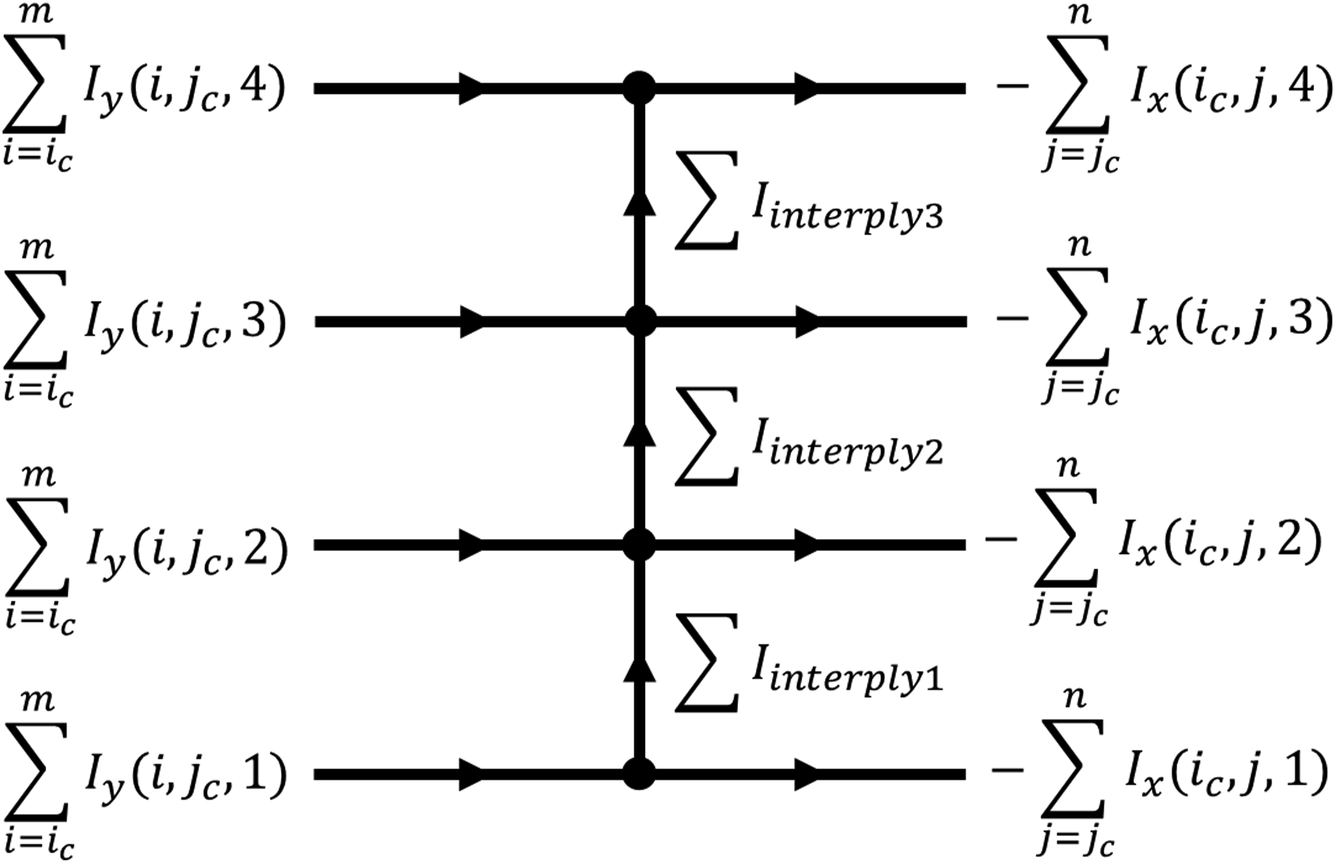
In the model only the first quadrant is simulated and therefore the symmetry condition is implemented according to the boundary condition, equation (34), where k is the ply-number and a is an integer representing the j:th coordinate for I _x and the i:th coordinate for I _y . The element position (i _c , j_c) is the centre position of the coil in the plane. From this computation the whole image can be extracted easily by just mirroring the computed quadrant along the symmetry planes (the dashed white lines in Figure 13) and adjust the signs of the current components.

$$I_x\left(i_c,a,k\right)=-I_y\left(a,j_c,k\right)$$

(34)

Thermal model

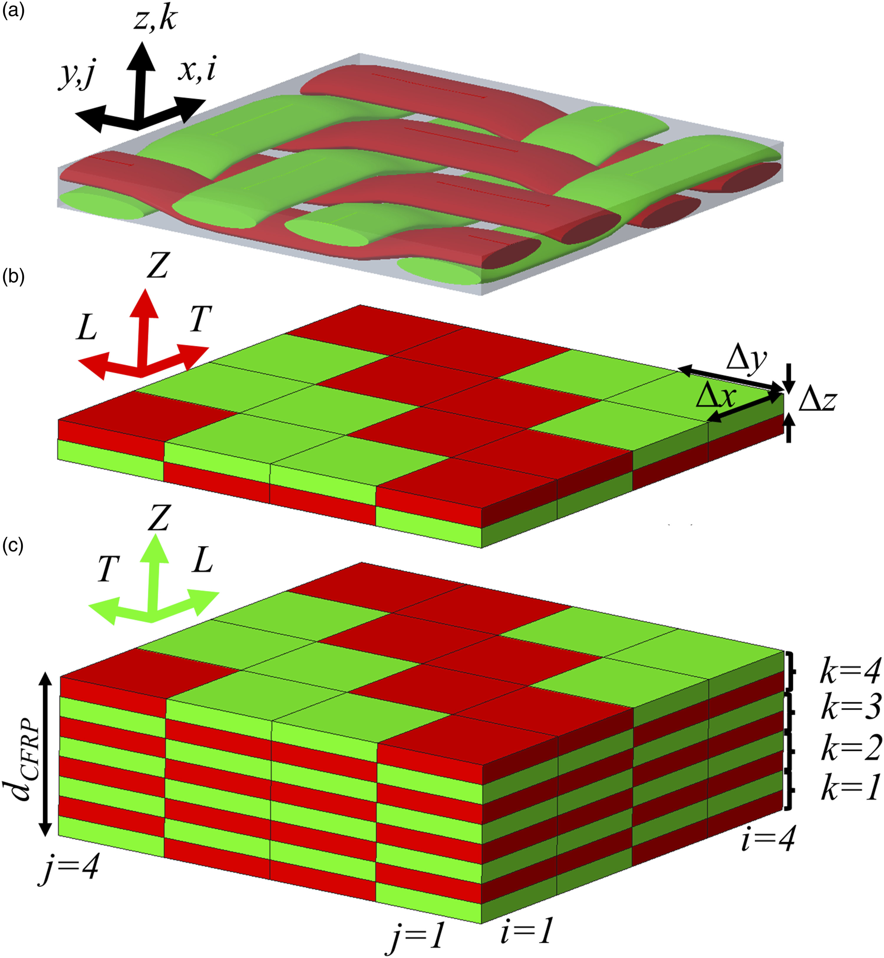
Discrete volume element representation

Each element from the resistor network is represented with two discrete volume elements in the thermal model as described in Figure 15; volume elements representing the tows along the x-axis (green) are denoted (i,j,k,t) _x where t is the time, and volume elements representing the tows along the y-axis, are denoted (i,j,k,t) _y . In this context the letters L, T and Z are used to describe the fibre directions on the volume element level; L represents the along fibre direction, T represents the transverse fibre in-plane direction and Z represents the through thickness direction. Temperature of the respective volume elements at the timestamp t are denoted T (i,j,k,t) _x and T (i,j,k,t) _y . Each volume element has the thickness Δz according to equation (35). Figure 15(c) shows how plies are stacked to represent plates with multiple plies. The synchronization of the relative position between adjacent plies, i.e. the fact that red domains are always adjacent to green domains in z-direction, are of course very difficult to achieve in an industrial manufacturing process, but it is considered a good approximation, since the relative positioning of fabric plies will be randomly distributed, with a rapid temperature equalization through the thickness, as explained by Lundström et al. 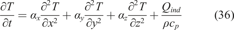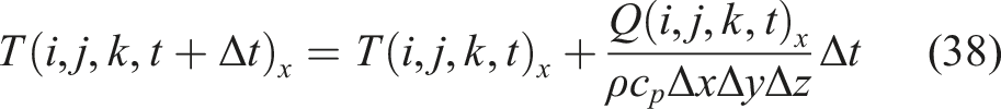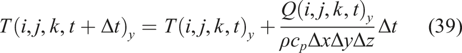²² The temperature distribution in three dimensions is governed by the heat equation (36) where α is the thermal diffusivity, ρ is the density, c _p is the specific heat capacity and Q (W/m³) represents the heating power source. The relationship between thermal diffusivity α and thermal conductivity λ is according to equation (37). The finite difference method FTCS (Forward time centred space) is used to solve the heat equation. 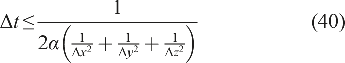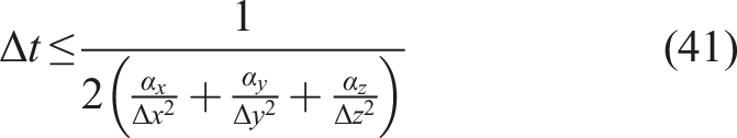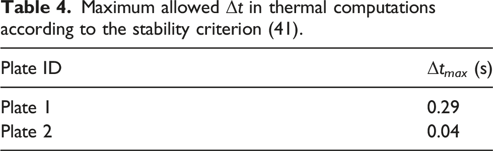The discretized heat equation (38), for computation of T (i,j,k,t) _x and equation (39), for computation of T (i,j,k,t) _y are used to calculate the temperature field at the timestep Δt forward in time, using MATLAB. 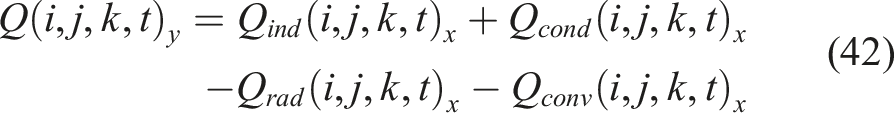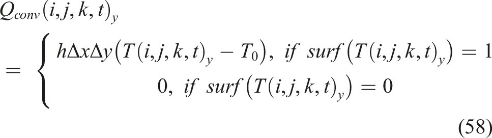The timestep Δt must be selected so that the stability criterion equation (40), Eftring, ²⁵ is fulfilled. For the case with direction dependent diffusivity the criterion can be expressed according to equation (41). In order to distinguish between the heat loss in the resistor network, which is denoted by the letter P, and the heat flow in the volume elements, the letter Q is used in the thermal model, although with the same unit, [W]. Q (i,j,k,t) _x and Q (i,j,k,t) _y represent the total heat flow [W] into a respective volume element at the time t according to equations (42) and (43) where the subscript ind stands for induced power, cond stands for conducted power, conv stands for convective heat loss and rad stands for radiative heat loss. The thermal calculations are made for the whole plate, not just one fourth, since the twill-structure does not allow the thermal problem to be reduced to just one fourth of the geometry. The computation of the temperature for each volume element is according to equations (38) and (39), thus no matrix inversions are involved and the computation complexity depends linearly on the number of elements and the number of timesteps.

$$\mathrm{\Delta }z=\frac{d_{CFRP}}{2N_{plies}}$$

(35)

$$\frac{\partial T}{\partial t}={\alpha }_x\frac{{\partial }^{2}T}{\partial x^2}+{\alpha }_y\frac{{\partial }^{2}T}{\partial y^2}+{\alpha }_z\frac{{\partial }^{2}T}{\partial z^2}+\frac{Q_{ind}}{\rho c_p}$$

(36)

$$\alpha =\frac{\lambda }{\rho c_p}$$

(37)

$$T{\left(i,j,k,t+\mathrm{\Delta }t\right)}_x=T{\left(i,j,k,t\right)}_x+\frac{Q{\left(i,j,k,t\right)}_x}{\rho c_p\mathrm{\Delta }x\mathrm{\Delta }y\mathrm{\Delta }z}\mathrm{\Delta }t$$

(38)

$$T{\left(i,j,k,t+\mathrm{\Delta }t\right)}_y=T{\left(i,j,k,t\right)}_y+\frac{Q{\left(i,j,k,t\right)}_y}{\rho c_p\mathrm{\Delta }x\mathrm{\Delta }y\mathrm{\Delta }z}\mathrm{\Delta }t$$

(39)

$$\mathrm{\Delta }t\le \frac{1}{2\alpha \left(\frac{1}{\mathrm{\Delta }{x}^2}+\frac{1}{\mathrm{\Delta }{y}^2}+\frac{1}{\mathrm{\Delta }{z}^2}\right)}$$

(40)

$$\mathrm{\Delta }t\le \frac{1}{2\left(\frac{{\alpha }_x}{\mathrm{\Delta }{x}^2}+\frac{{\alpha }_y}{\mathrm{\Delta }{y}^2}+\frac{{\alpha }_z}{\mathrm{\Delta }{z}^2}\right)}$$

(41)

$$Q{\left(i,j,k,t\right)}_y=Q_{ind}{\left(i,j,k,t\right)}_x+Q_{cond}{\left(i,j,k,t\right)}_x-Q_{rad}{\left(i,j,k,t\right)}_x-Q_{conv}{\left(i,j,k,t\right)}_x$$

(42)

$$Q{\left(i,j,k,t\right)}_y=Q_{ind}{\left(i,j,k,t\right)}_y+Q_{cond}{\left(i,j,k,t\right)}_y-Q_{rad}{\left(i,j,k,t\right)}_y-Q_{conv}{\left(i,j,k,t\right)}_y$$

(43)

Figure 15.

A twill fabric ply is represented with discrete homogeneous volume elements in the thermal model. (a) Illustration of a twill ply. x-directional tows are green and y-directional tows are red in order to clarify the simplification. (b) Simplification of the twill ply to discrete homogeneous volume elements in the model. (c) Simplified layers are stacked in the case of multiple fabric plies (in this case four plies). Ply k = 1 is the ply closest to the coil.

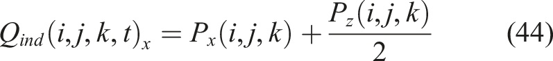
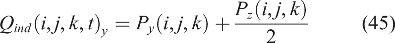
The heating power induced in each resistor, computed by the resistor network model, is distributed into the volume elements. The power P _x (i,j,k) is assigned to the volume element (i,j,k,t) _x and P _y (i,j,k) is assigned to the volume element (i,j,k,t) _y . The power P _z (i,j,k) generated along the R _z resistors are not associated with a well-defined volume since the heat generated along R _z is generated both within the tows and in the contact between crossing tows. Therefore, the heat generation P_z (i,j,k) is equally divided to the volume elements (i,j,k,t) _x and (i,j,k,t) _y so that the induced power in the volume elements are computed according to equations (44) and (45). This is a reasonable approximation due to the rapid temperature equalization within the thin layers as observed by Lundström et al. ¹²

$$Q_{ind}{\left(i,j,k,t\right)}_x=P_x\left(i,j,k\right)+\frac{P_z\left(i,j,k\right)}{2}$$

(44)

$$Q_{ind}{\left(i,j,k,t\right)}_y=P_y\left(i,j,k\right)+\frac{P_z\left(i,j,k\right)}{2}$$

(45)

The volume elements are thermally connected to each other in the z direction according to Figure 15, and to preserve the thermal conduction along the fibre direction (the direction with highest thermal diffusivity) volume elements with the same colour are connected to each other in the L direction (along fibre). This means that the volume element (i,j,k,t) _x always have the neighbours (i-1,j,k,t) _x and (i + 1,j,k,t) _x in the L direction and the volume element (i,j,k,t) _y always have the neighbours (i,j-1,k,t) _y and (i,j + 1,k,t) _y in the L direction. 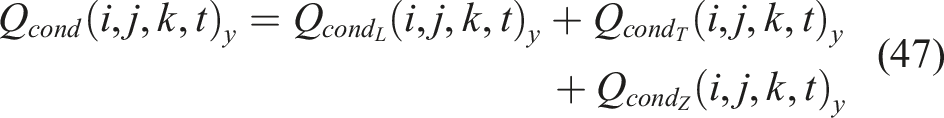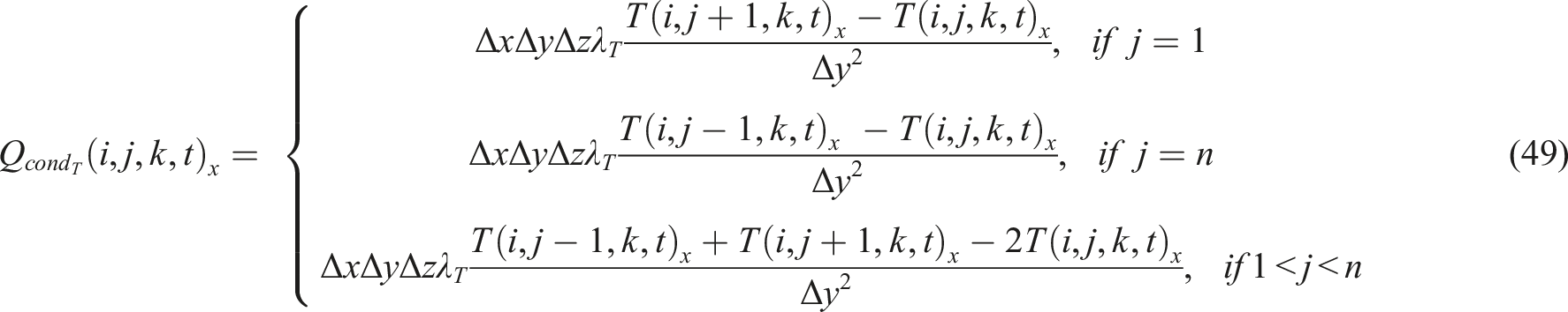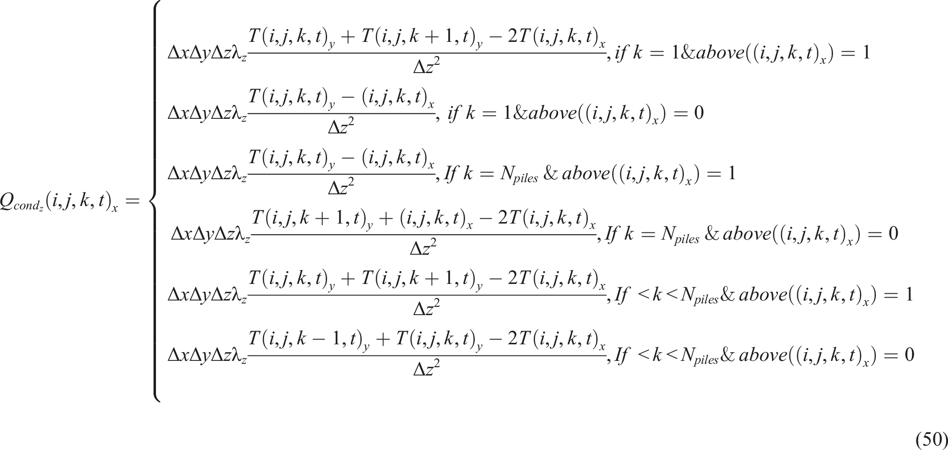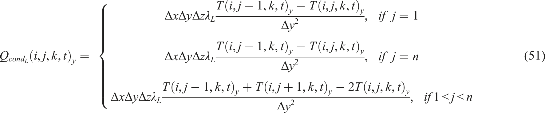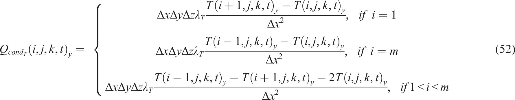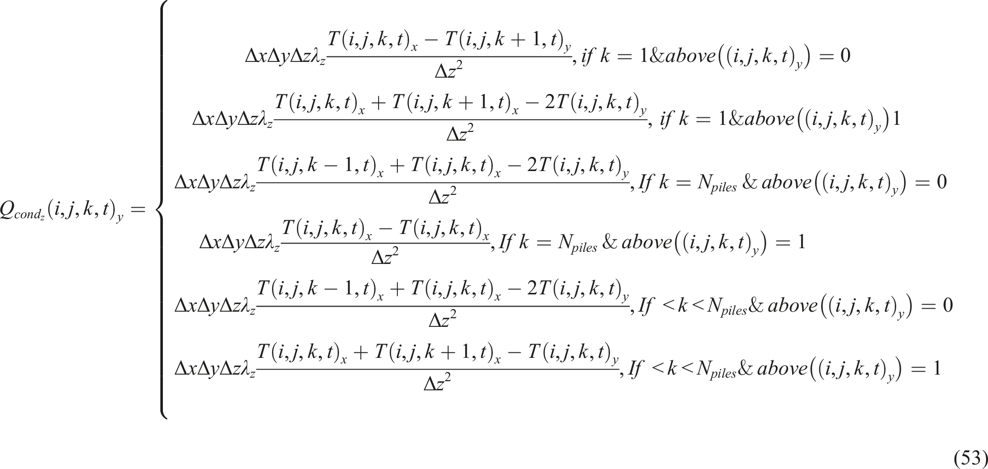Consequently, to preserve the effective macroscopic diffusivity in the plane directions, (i,j,k,t) _x always have the neighbours (i,j − 1,k,t) _x and (i,j + 1,k,t) _x in the T direction (transverse the fibre direction in-plane) and the volume element (i,j,k,t) _y always have the neighbours (i−1,j,k,t) _y and (i + 1,j,k,t) _y in the T direction. Based on the mentioned approximations the heat conduction is calculated according to equations (46) and (47) where each component are calculated according to equations (48)–(53). The subscript cond _L denotes the heat conduction in L direction, cond _T denotes the heat conduction in T direction and cond _Z denotes the heat conduction in Z direction. The letters m and n represent the number of elements in x and y directions respectively. In these equations the function (54) is used to determine if the volume element (i,j,k,t) _x placed above (i,j,k,t) _y or vice versa.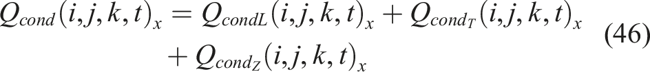

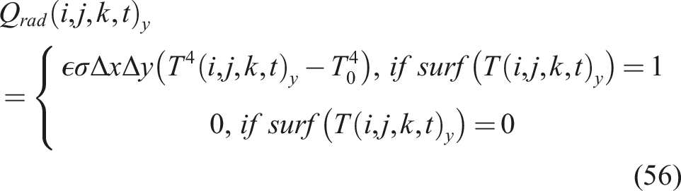
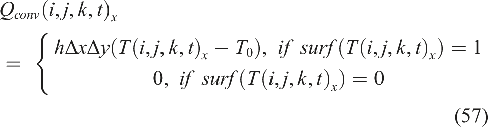
$$Q_{cond}{\left(i,j,k,t\right)}_x=Q_{condL}{\left(i,j,k,t\right)}_x+Q_{con{d}_T}{\left(i,j,k,t\right)}_x+Q_{con{d}_Z}{\left(i,j,k,t\right)}_x$$

(46)

$$Q_{cond}{\left(i,j,k,t\right)}_y=Q_{con{d}_L}{\left(i,j,k,t\right)}_y+Q_{con{d}_T}{\left(i,j,k,t\right)}_y+Q_{con{d}_Z}{\left(i,j,k,t\right)}_y$$

(47)

$$Q_{con{d}_L}{\left(i,j,k,t\right)}_x= \{\begin{array}{c}\mathrm{\Delta }x\mathrm{\Delta }y\mathrm{\Delta }z{\lambda }_L\frac{T{\left(i+1,j,k,t\right)}_x-T{\left(i,j,k,t\right)}_x}{\mathrm{\Delta }{x}^2}, if i=1\\ \mathrm{\Delta }x\mathrm{\Delta }y\mathrm{\Delta }z{\lambda }_L\frac{T{\left(i-1,j,k,t\right)}_x-T{\left(i,j,k,t\right)}_x}{\mathrm{\Delta }{x}^2}, if i=m\\ \mathrm{\Delta }x\mathrm{\Delta }y\mathrm{\Delta }z{\lambda }_L\frac{T{\left(i-1,j,k,t\right)}_x+T{\left(i+1,j,k,t\right)}_x-2T{\left(i,j,k,t\right)}_x}{\mathrm{\Delta }{x}^2}, if1<i<m\end{array}$$

(48)

$$Q_{con{d}_T}{\left(i,j,k,t\right)}_x= \{\begin{array}{c}\mathrm{\Delta }x\mathrm{\Delta }y\mathrm{\Delta }z{\lambda }_T\frac{T{\left(i,j+1,k,t\right)}_x-T{\left(i,j,k,t\right)}_x}{\mathrm{\Delta }{y}^2}, if j=1\\ \mathrm{\Delta }x\mathrm{\Delta }y\mathrm{\Delta }z{\lambda }_T\frac{T{\left(i,j-1,k,t\right)}_x -T{\left(i,j,k,t\right)}_x}{\mathrm{\Delta }{y}^2}, if j=n\\ \mathrm{\Delta }x\mathrm{\Delta }y\mathrm{\Delta }z{\lambda }_T\frac{T{\left(i,j-1,k,t\right)}_x+T{\left(i,j+1,k,t\right)}_x-2T{\left(i,j,k,t\right)}_x}{\mathrm{\Delta }{y}^2}, if1<j<n\end{array}$$

(49)

$$\begin{array}{l}{Q}_{con{d}_z}{\left(i,j,k,t\right)}_x=\{\begin{array}{l}\mathrm{\Delta }x\mathrm{\Delta }y\mathrm{\Delta }z{\text{λ}}_z\frac{T{\left(i,j,k,t\right)}_y+T{\left(i,j,k+1,t\right)}_y-2T{\left(i,j,k,t\right)}_x}{\mathrm{\Delta }{z}^2},if\hspace{0.17em}k=1\&above\left({\left(i,j,k,t\right)}_x\right)=1\\ \mathrm{\Delta }x\mathrm{\Delta }y\mathrm{\Delta }z{\text{λ}}_z\frac{T{\left(i,j,k,t\right)}_y-{\left(i,j,k,t\right)}_x}{\mathrm{\Delta }{z}^2},\hspace{0.17em}if\hspace{0.17em}k=1\&above\left({\left(i,j,k,t\right)}_x\right)=0\\ \mathrm{\Delta }x\mathrm{\Delta }y\mathrm{\Delta }z{\text{λ}}_z\frac{T{\left(i,j,k,t\right)}_y-{\left(i,j,k,t\right)}_x}{\mathrm{\Delta }{z}^2},If\hspace{0.17em}k=N_{piles}\hspace{0.17em}\&\hspace{0.17em}above\left({\left(i,j,k,t\right)}_x\right)=1\\ \hspace{0.17em}\mathrm{\Delta }x\mathrm{\Delta }y\mathrm{\Delta }z{\text{λ}}_z\frac{T{\left(i,j,k+1,t\right)}_y+{\left(i,j,k,t\right)}_x-2T{\left(i,j,k,t\right)}_x}{\mathrm{\Delta }{z}^2},If\hspace{0.17em}k=N_{piles}\hspace{0.17em}\&\hspace{0.17em}above\left({\left(i,j,k,t\right)}_x\right)=0\\ \mathrm{\Delta }x\mathrm{\Delta }y\mathrm{\Delta }z{\text{λ}}_z\frac{T{\left(i,j,k,t\right)}_y+T{\left(i,j,k+1,t\right)}_y-2T{\left(i,j,k,t\right)}_x}{\mathrm{\Delta }{z}^2},If\hspace{0.17em}<k<N_{piles}\&\hspace{0.17em}above\left({\left(i,j,k,t\right)}_x\right)=1\\ \mathrm{\Delta }x\mathrm{\Delta }y\mathrm{\Delta }z{\text{λ}}_z\frac{T{\left(i,j,k-1,t\right)}_y+T{\left(i,j,k,t\right)}_y-2T{\left(i,j,k,t\right)}_x}{\mathrm{\Delta }{z}^2},If\hspace{0.17em}<k<N_{piles}\&\hspace{0.17em}above\left({\left(i,j,k,t\right)}_x\right)=0\end{array}\hspace{0.17em}\\ \end{array}$$

(50)

$$Q_{con{d}_L}{\left(i,j,k,t\right)}_y= \{\begin{array}{c}\mathrm{\Delta }x\mathrm{\Delta }y\mathrm{\Delta }z{\lambda }_L\frac{T{\left(i,j+1,k,t\right)}_y-T{\left(i,j,k,t\right)}_y}{\mathrm{\Delta }{y}^2}, if j=1\\ \mathrm{\Delta }x\mathrm{\Delta }y\mathrm{\Delta }z{\lambda }_L\frac{T{\left(i,j-1,k,t\right)}_y-T{\left(i,j,k,t\right)}_y}{\mathrm{\Delta }{y}^2}, if j=n\\ \mathrm{\Delta }x\mathrm{\Delta }y\mathrm{\Delta }z{\lambda }_L\frac{T{\left(i,j-1,k,t\right)}_y+T{\left(i,j+1,k,t\right)}_y-2T{\left(i,j,k,t\right)}_y}{\mathrm{\Delta }{y}^2}, if1<j<n\end{array}$$

(51)

$$Q_{con{d}_T}{\left(i,j,k,t\right)}_y= \{\begin{array}{c}\mathrm{\Delta }x\mathrm{\Delta }y\mathrm{\Delta }z{\lambda }_T\frac{T{\left(i+1,j,k,t\right)}_y-T{\left(i,j,k,t\right)}_y}{\mathrm{\Delta }{x}^2}, if i=1\\ \mathrm{\Delta }x\mathrm{\Delta }y\mathrm{\Delta }z{\lambda }_T\frac{T{\left(i-1,j,k,t\right)}_y-T{\left(i,j,k,t\right)}_y}{\mathrm{\Delta }{x}^2}, if i=m\\ \mathrm{\Delta }x\mathrm{\Delta }y\mathrm{\Delta }z{\lambda }_T\frac{T{\left(i-1,j,k,t\right)}_y+T{\left(i+1,j,k,t\right)}_y-2T{\left(i,j,k,t\right)}_y}{\mathrm{\Delta }{x}^2}, if1<i<m\end{array}$$

(52)

$$\begin{array}{l}{Q}_{con{d}_z}{\left(i,j,k,t\right)}_y=\{\begin{array}{l}\hspace{0.17em}\hspace{0.17em}\hspace{0.17em}\hspace{0.17em}\hspace{0.17em}\hspace{0.17em}\hspace{0.17em}\hspace{0.17em}\hspace{0.17em}\hspace{0.17em}\hspace{0.17em}\hspace{0.17em}\hspace{0.17em}\hspace{0.17em}\hspace{0.17em}\hspace{0.17em}\hspace{0.17em}\hspace{0.17em}\hspace{0.17em}\hspace{0.17em}\mathrm{\Delta }x\mathrm{\Delta }y\mathrm{\Delta }z{\lambda }_z\frac{T{\left(i,j,k,t\right)}_x-T{(i,j,k+1,t)}_y}{\mathrm{\Delta }{z}^2},if\hspace{0.17em}k=1\&above\left({\left(i,j,k,t\right)}_y\right)=0\\ \hspace{0.17em}\hspace{0.17em}\hspace{0.17em}\hspace{0.17em}\hspace{0.17em}\mathrm{\Delta }x\mathrm{\Delta }y\mathrm{\Delta }z{\lambda }_z\frac{T{\left(i,j,k,t\right)}_x+T{(i,j,k+1,t)}_x-2T{\left(i,j,k,t\right)}_y}{\mathrm{\Delta }{z}^2},\hspace{0.17em}if\hspace{0.17em}k=1\&above\left({\left(i,j,k,t\right)}_y\right)1\\ \mathrm{\Delta }x\mathrm{\Delta }y\mathrm{\Delta }z{\lambda }_z\frac{T{\left(i,j,k-1,t\right)}_x+T{\left(i,j,k,t\right)}_x-2T{\left(i,j,k,t\right)}_y}{\mathrm{\Delta }{z}^2},If\hspace{0.17em}k=N_{piles}\hspace{0.17em}\&\hspace{0.17em}above\left({\left(i,j,k,t\right)}_y\right)=0\\ \hspace{0.17em}\hspace{0.17em}\hspace{0.17em}\hspace{0.17em}\hspace{0.17em}\hspace{0.17em}\hspace{0.17em}\mathrm{\Delta }x\mathrm{\Delta }y\mathrm{\Delta }z{\lambda }_z\frac{T{\left(i,j,k,t\right)}_x-T{\left(i,j,k,t\right)}_x}{\mathrm{\Delta }{z}^2},If\hspace{0.17em}k=N_{piles}\hspace{0.17em}\&\hspace{0.17em}above\left({\left(i,j,k,t\right)}_y\right)=1\\ \mathrm{\Delta }x\mathrm{\Delta }y\mathrm{\Delta }z{\lambda }_z\frac{T{\left(i,j,k-1,t\right)}_x+T{(i,j,k,t)}_x-2T{(i,j,k,t)}_y}{\mathrm{\Delta }{z}^2},If\hspace{0.17em}<k<N_{piles}\&\hspace{0.17em}above\left({\left(i,j,k,t\right)}_y\right)=0\\ \mathrm{\Delta }x\mathrm{\Delta }y\mathrm{\Delta }z{\lambda }_z\frac{T{\left(i,j,k,t\right)}_x+T{\left(i,j,k+1,t\right)}_x-T{\left(i,j,k,t\right)}_y}{\mathrm{\Delta }{z}^2},If\hspace{0.17em}<k<N_{piles}\&\hspace{0.17em}above\left({\left(i,j,k,t\right)}_y\right)=1\end{array}\hspace{0.17em}\\ \end{array}$$

(53)

$$above\left({\left(i,j,k,t\right)}_x\right)=\{\begin{array}{c}1,ifthevolumeelement{\left(i,j,k,t\right)}_{x}isplacedabove{\left(i,j,k,t\right)}_y\\ 0,ifthevolumeelement{\left(i,j,k,t\right)}_{x}isplacedbelow{\left(i,j,k,t\right)}_y\end{array}$$

(54)

The radiative surface heat loss from the horizontal surfaces is computed according to equations (55) and (56) (the temperature must be provided in Kelvin) where the emissivity ϵ = 0.93, as previously mentioned. The convective heat loss is computed according to equations (57) and (58). The function (59) is used to determine if the volume element is a surface volume element, i.e. in contact with the surrounding air. Convective and radiative heat losses from the vertical edges of the plates are disregarded. The thermographic recordings during induction heating was performed in a location with no ventilation and thus only natural convection occurred. In the model the convective heat transfer coefficient was set to h = 10 W/(m²∙ K) as in the work by et al. ¹⁴ and the works by Lundström et al.^20,22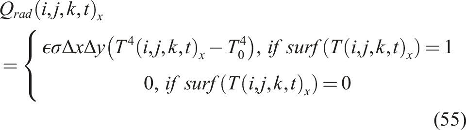

$$Q_{rad}{(i,j,k,t)}_x=\{\begin{array}{c}\mathit{ϵ}\sigma \mathrm{\Delta }x\mathrm{\Delta }y\left(T^4{\left(i,j,k,t\right)}_x-T_0^4\right),ifsurf\left(T{\left(i,j,k,t\right)}_x\right)=1\\ 0,ifsurf\left(T{\left(i,j,k,t\right)}_x\right)=0\end{array}$$

(55)

$$Q_{rad}{\left(i,j,k,t\right)}_y=\{\begin{array}{c}\mathit{ϵ}\sigma \mathrm{\Delta }x\mathrm{\Delta }y\left(T^4{\left(i,j,k,t\right)}_y-T_0^4\right),ifsurf\left(T{\left(i,j,k,t\right)}_y\right)=1\\ 0,ifsurf\left(T{\left(i,j,k,t\right)}_y\right)=0\end{array}$$

(56)

$$Q_{conv}{\left(i,j,k,t\right)}_x=\{\begin{array}{c}h\mathrm{\Delta }x\mathrm{\Delta }y\left(T{\left(i,j,k,t\right)}_x-T_0\right),ifsurf\left(T{\left(i,j,k,t\right)}_x\right)=1\\ 0,ifsurf\left(T{\left(i,j,k,t\right)}_x\right)=0\end{array}$$

(57)

$$Q_{conv}{\left(i,j,k,t\right)}_y=\{\begin{array}{c}h\mathrm{\Delta }x\mathrm{\Delta }y\left(T{\left(i,j,k,t\right)}_y-T_0\right),ifsurf\left(T{\left(i,j,k,t\right)}_y\right)=1\\ 0,ifsurf\left(T{\left(i,j,k,t\right)}_y\right)=0\end{array}$$

(58)

$$surf\left({\left(i,j,k,t\right)}_x\right)=\{\begin{array}{c}1,ifthevolumeelement{\left(i,j,k,t\right)}_{x}isasurfacevolumeelement\\ 0,ifthevolumeelement{\left(i,j,k,t\right)}_{x}isnotasurfacevolumeelement\end{array}$$

(59)

Thermal conductivity and specific heat capacity

The diffusivity and specific heat capacity were characterized by Lundström et al. ²² (The same CFRP plates were used in this study) who found that these properties depend on the fibre volume fraction according to equations (60)–(62). Equation (60) shows how the diffusivity in the z-direction depends on the fibre volume fraction ϕ, equation (61) shows how the in-plane diffusivity (either x, or y direction) depends on ϕ and equation (62) shows how the specific heat capacity depends on ϕ. The measurements by Lundström et al. ²² were performed on woven CFRP and therefore the thermal conductivity along and transverse fibre direction could not be measured explicitly. However due to the “rule o mixtures” the effective value of the macroscopic thermal conductivity component λ _X relates to λ _L and λ _T equation (63), and λ _L relates the fibre conductivity λ _f and the matric conductivity λ _m according to according to equation (64), as proposed by Lundström et al. ²² Thus, since λ _X , λ _f ,λ _m and ϕ are known λ _L and λ _T can be determined. Based on the presented thermal properties the stability criterion, equation (41), can be used to calculate maximum allowed timestep Δt in the computations of the temperature distribution. The maximum allowed timesteps are presented in Table 4.

$${\alpha }_Z=0.1469e^{2.343\varphi }\left[{\text{mm}}^2/\text{s}\right]$$

(60)

$${\alpha }_X=4.056\varphi -0.2186\left[{\text{ mm}}^2/\text{s}\right]$$

(61)

$$c_p=-0.7954\varphi +1.463\left[\text{ kJ}/\left(\text{kg}\cdot \text{K}\right)\right]$$

(62)

$${\lambda }_X=0.5{\lambda }_L+0.5{\lambda }_T$$

(63)

$${\lambda }_L=\varphi {\lambda }_f+\left(1-\varphi \right){\lambda }_m$$

(64)

Table 4.

Maximum allowed Δt in thermal computations according to the stability criterion (41).

Plate ID	Δt max (s)
Plate 1	0.29
Plate 2	0.04

Results and discussion

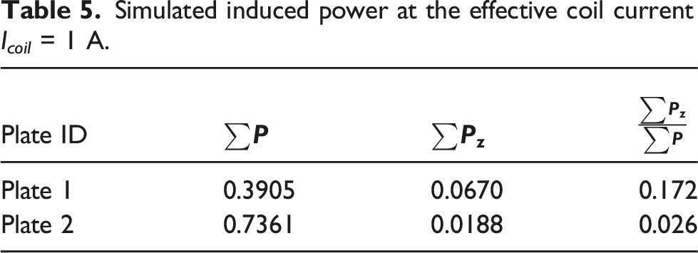
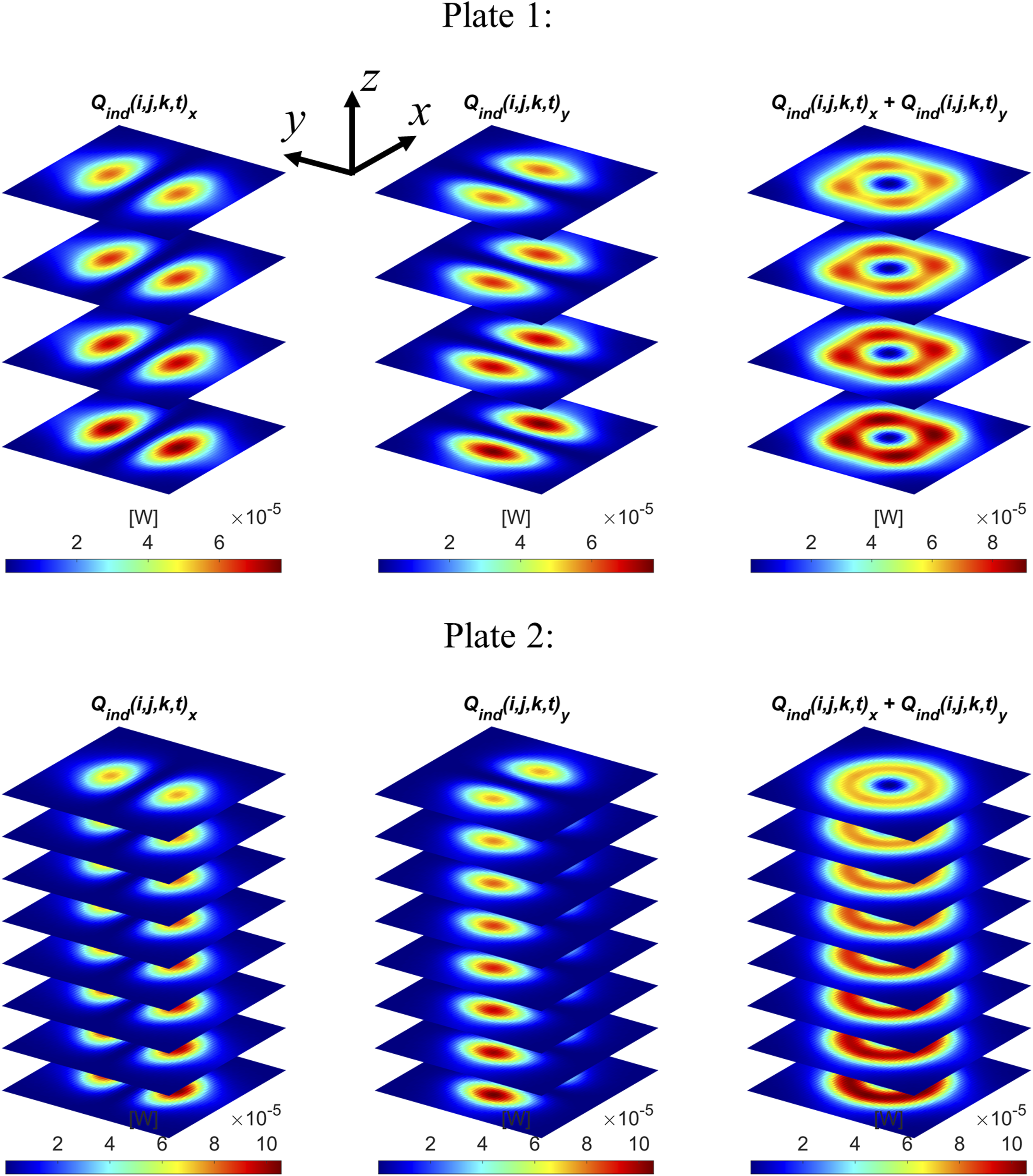
The first step in the simulation is to compute the discrete current components using the resistor network model. Figure 16 shows the simulated current and the heating power generation per resistor in plate 1 (each pixel corresponds to the current or heating power in a discrete resistor). According to the simulation results, most of the heat generation occurs along the fibre directions (x or y direction), as shown in Table 5. However, the heat generation along the z direction is significantly higher in plate 1 than in plate 2; 17.2% in plate 1 compared to 2.6% in plate 2 which is due to the significantly higher value of R _z in plate 1. In the next step the computed heating power is used in the thermal model to compute the temperature distribution. Figure 17 shows the simulated heating power per volume element in plate 1 and 2; the first column shows the distribution of the induced power in the x-directional tow volume elements Q _ind (i,j,k,t) _x and the second column shows the corresponding distribution for the y-directional tow volume elements Q _ind (i,j,k,t) _y . The third column shows the sum of the x- and y directional volume elements, Q _ind (i,j,k,t) _x + Q _ind (i,j,k,t) _y , which gives an indication of the relative temperature distribution when the heating power has diffused between x directional and y directional fibre tows. In plate 2 this results in a circular distribution, but in plate 1 hotspots appear in four positions similar to the distribution of P _z , which agrees with the results by Lundström et al. ²² The frequency of the coil current is 60 kHz in each case and the level of the coil current for each case is stated in the captions for the figures presenting the measured and simulated temperature distributions.

Figure 16.

The first upper row shows the effective value of the current flowing in each resistor and the bottom row show the resulting heat generation per resistor in CFRP plate 1. The effective coil current is I _coil = 1 A. The plies are arranged so that the bottom ply is closest to the coil.

Table 5.

Simulated induced power at the effective coil current I _coil = 1 A.

Plate ID	${{\displaystyle \sum }}^{\text{}}\mathit{P}$	${{\displaystyle \sum }}^{\text{}}{\mathit{P}}_{\mathit{z}}$	$\frac{{{\displaystyle \sum }}^{\text{}}{\mathit{P}}_{\mathit{z}}}{{{\displaystyle \sum }}^{\text{}}\mathit{P}}$
Plate 1	0.3905	0.0670	0.172
Plate 2	0.7361	0.0188	0.026

Figure 17.

Simulated induced power distribution in plate one and plate 2. The power presented is the power per volume element. The effective coil current is I _coil = 1 A.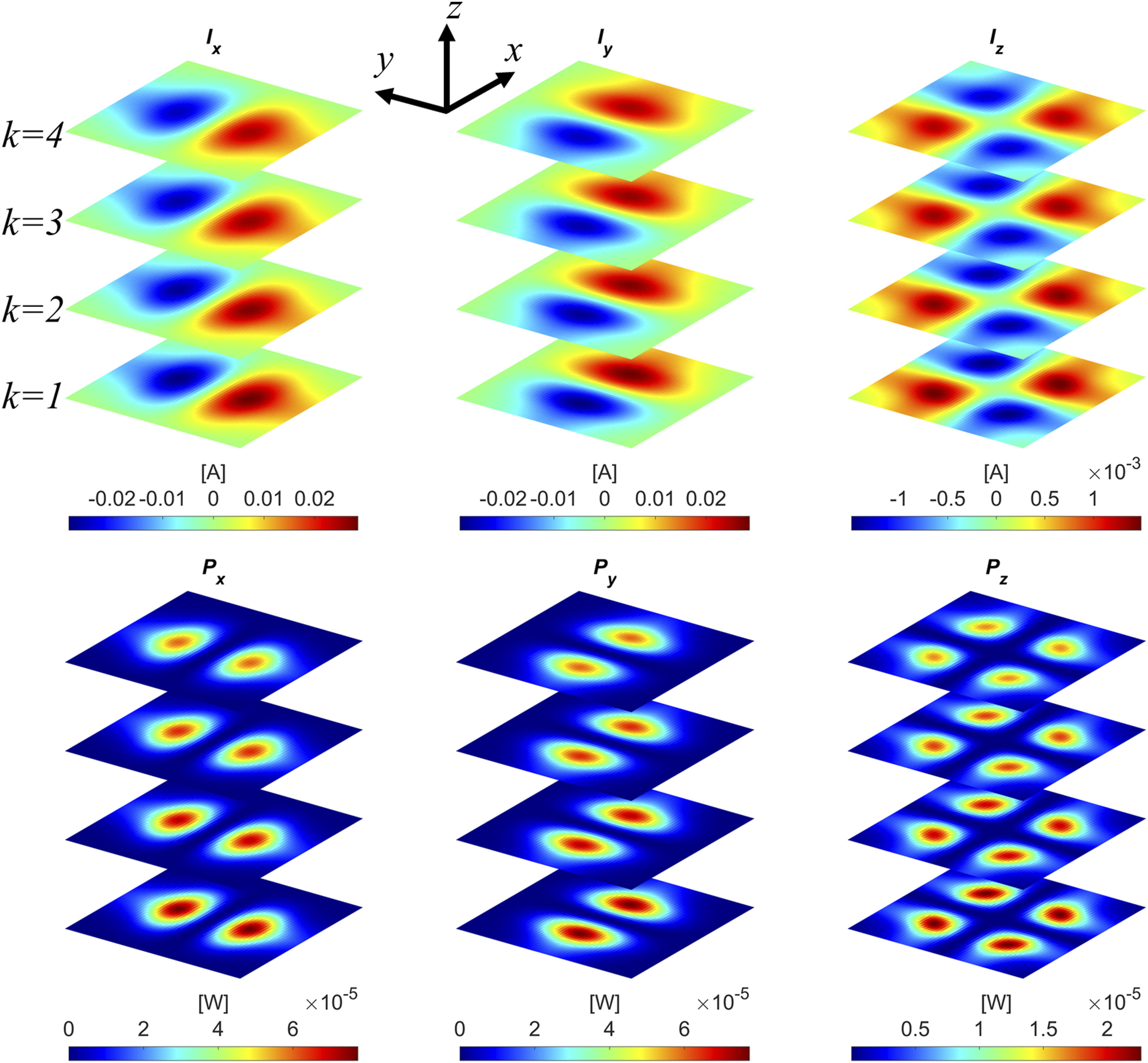

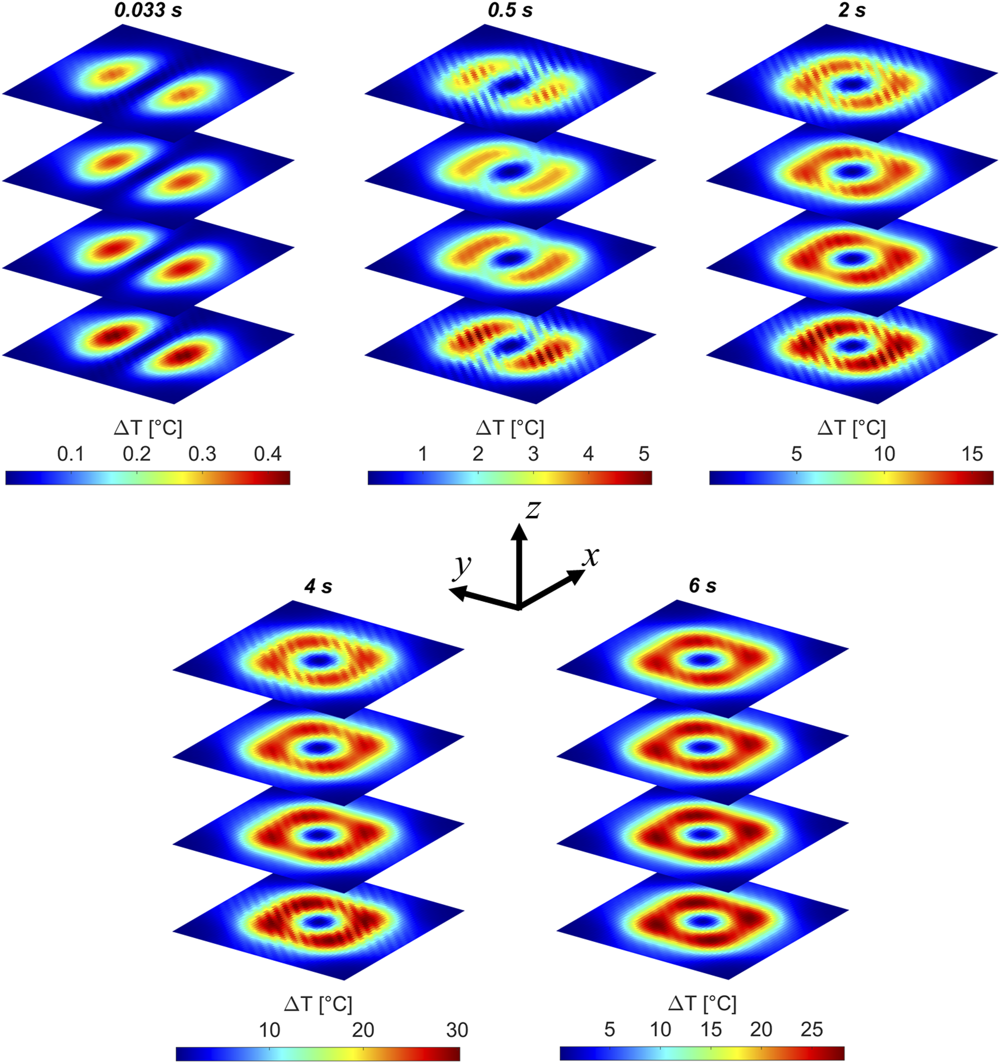
The temperature distributions are presented as the temperature increase ΔT from the start temperature T ₀ (21°C) to the temperature distribution T at time t, equation (65). Figure 18 shows an example of the temperature T (i,j,k,t) _x for plate 1 (i.e., the red volume elements in Figure 15) at different timestamps during and after finished heating. It shows that at a very early timestamp (0.033 s) the distribution of T (i,j,k,t) _x gives a good indication of the distribution of Q _ind (i,j,k,t) _x . However, the heat rapidly diffuses from the y-directional fibres into the x-directional fibres, and vice versa, and the relative distribution looks more like the sum Q _ind (i,j,k,t) _x + Q _ind (i,j,k,t) _y in Figure 17. For computation of the initial temperature distributions, with a timestamp below 0.1 s, a time increment of Δt = 0.001 s was used, and for temperature distributions with a timestamp higher than 0.1 s the time increment Δt = 0.01 s was used. Both the used time increments are well within the stability range, Table 4.

$$\mathrm{\Delta }T=T-T_0$$

(65)

Figure 18.

The simulated temperature distribution in the T (i,j,k,t) _x volume elements for plate 1. The duration of the induction heating is 4 s. I _coil = 32.9 A.

Thermographic recordings were conducted during induction heating and compared with the simulated temperature distributions to validate the simulation model. Since the electrical and thermal properties are measured at room temperature (21–23°C) the thermographic induction heating was set to not exceed ΔT = 30°C (surface temperature). Within this interval it is considered a good approximation to use parameters measured at room temperature according to the measurements by Lundström et al. ²⁰ The comparisons between simulated and measured temperature are presented with the value δT _max presenting the relative difference between peak value in simulation and measurement according to equation (66), where ΔT _{s_max} is the peak temperature increase detected in the simulated temperature image and ΔT _{m_max} is the peak temperature increase detected in the measured temperature image. The thermographic measurements can only record the surface temperature and therefore need to be compared with the simulated surface temperature which is a combination of T (i,j,k,t) _x and T (i,j,k,t) _y according to Figure 15. Figure 19 shows T (i,j,k,t) _x and T (i,j,k,t) _y for ply 4 (the ply representing the front surface) from the same simulation as shown in Figure 18, and the resulting front surface temperature, due to the twill weave pattern, which is the pattern that can be compared to, and validated by the thermographic measurements.

$$\delta T_{max}=\frac{\mathrm{\Delta }{T}_{s_{max}}-\mathrm{\Delta }{T}_{m_{max}}}{\mathrm{\Delta }{T}_{m_{max}}}$$

(66)

Figure 19.

T (i,j,k,t)_x and T (i,j,k,t)_y for ply 4 (ply farthest away from the coil) are shown separately and combined in a twill pattern (as illustrated in Figure 15 and Figure 20), which gives the temperature of the front surface.

Figure 20.

(a) Photography of Plate two and the outer dimensions indicated. (b) Discretization into volume elements according to the principle described in Figure 15. The discrete coordinates (i and j) for the outer elements are indicated. The dimensions and number of tows are the same for plate 1.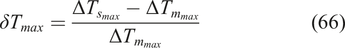

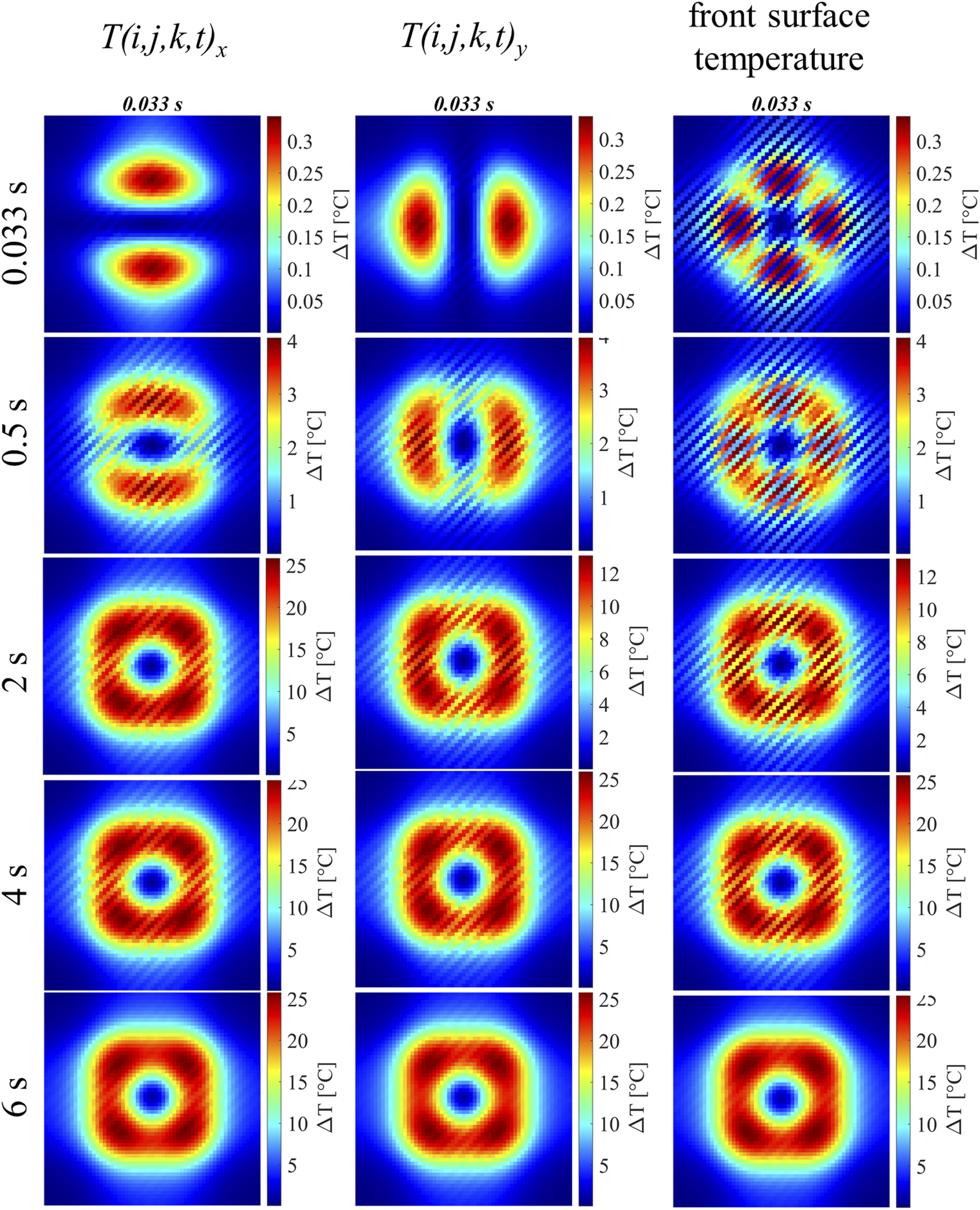
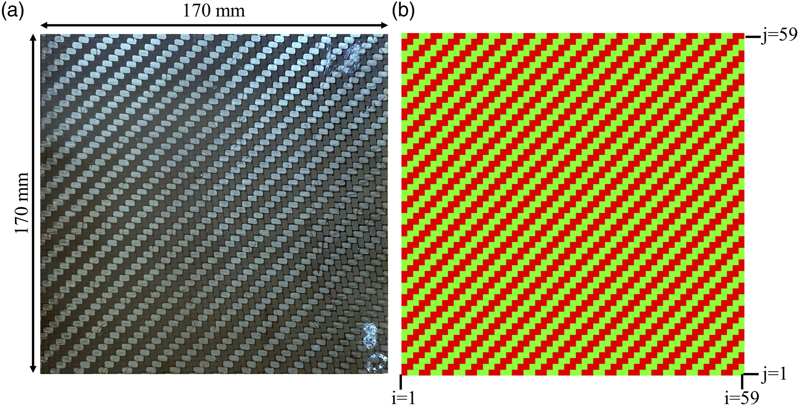
Figure 21 shows a comparison between simulation and thermographic measurement for the front surface, during and after induction heating. Figure 22 shows the corresponding comparison for the coil surface, which is only presented at the timestamp 6 s since the coil must be removed before that surface can be recorded. The current level was set to achieve approximately the same input power during all recordings. Figure 21 compares the temperature distribution between simulation and measurement for the front surface at five different timestamps. The induction heating duration is 4 s. Except for the first timestamp (0.033 s), plate 2 has an excellent agreement between simulation and measurement, with an deviation within just a few percents, regarding peak temperature, for both front surface and coil surface and therefore it is reasonable that the internal temperature also agrees with the model. For plate 1 the relative difference between measurement and simulation is larger but the pattern agrees well with the measurement. The initial timestamp (0.033 s) shows a significant dispersion for both cases. However, at the initial timestamp the absolute temperature increase is below 1°C which cannot be measured with high accuracy.

Figure 21.

Comparison between simulated and measured front surface temperature. The duration of the induction heating is 4s. The effective coil current for plate 1 is 32.9 A and 22.9 for plate 2. Using equation (30) the total induced power per plate can be calculated; 423 W in plate 1 and 386 W in plate 2. The temperature images and the coil currents are extracted from thermographic measurements presented by Lundström et al. ²²

Figure 22.

Comparison between simulated and measured coil surface temperature after 6 s. Duration of the induction heating is 4 s. The effective coil current is 33.4 A for plate 1 and 23.2 A for plate 2. Using equation (30) the induced power can be calculated; 436 W in plate 1 and 396 W in plate 2. The temperature images and the coil currents are extracted thermographic measurements as presented by Lundström et al. ²²

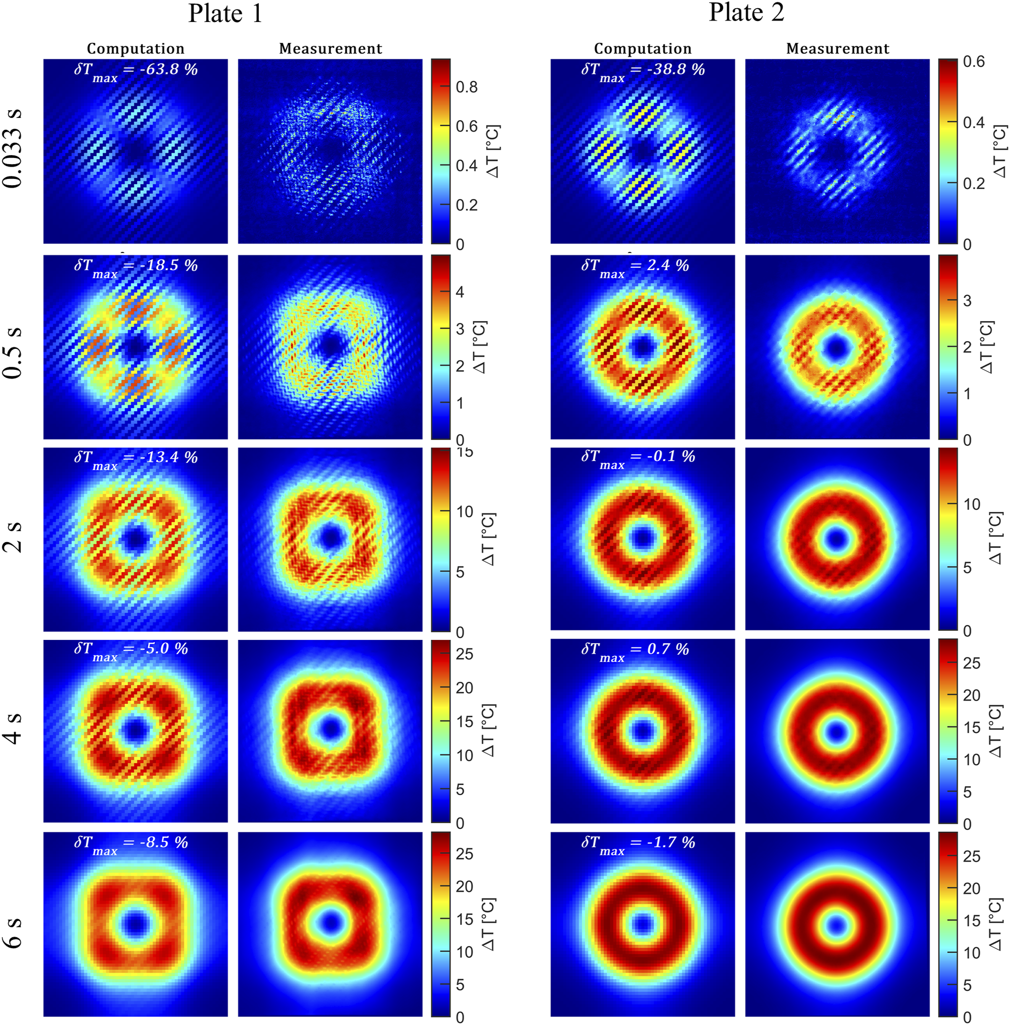
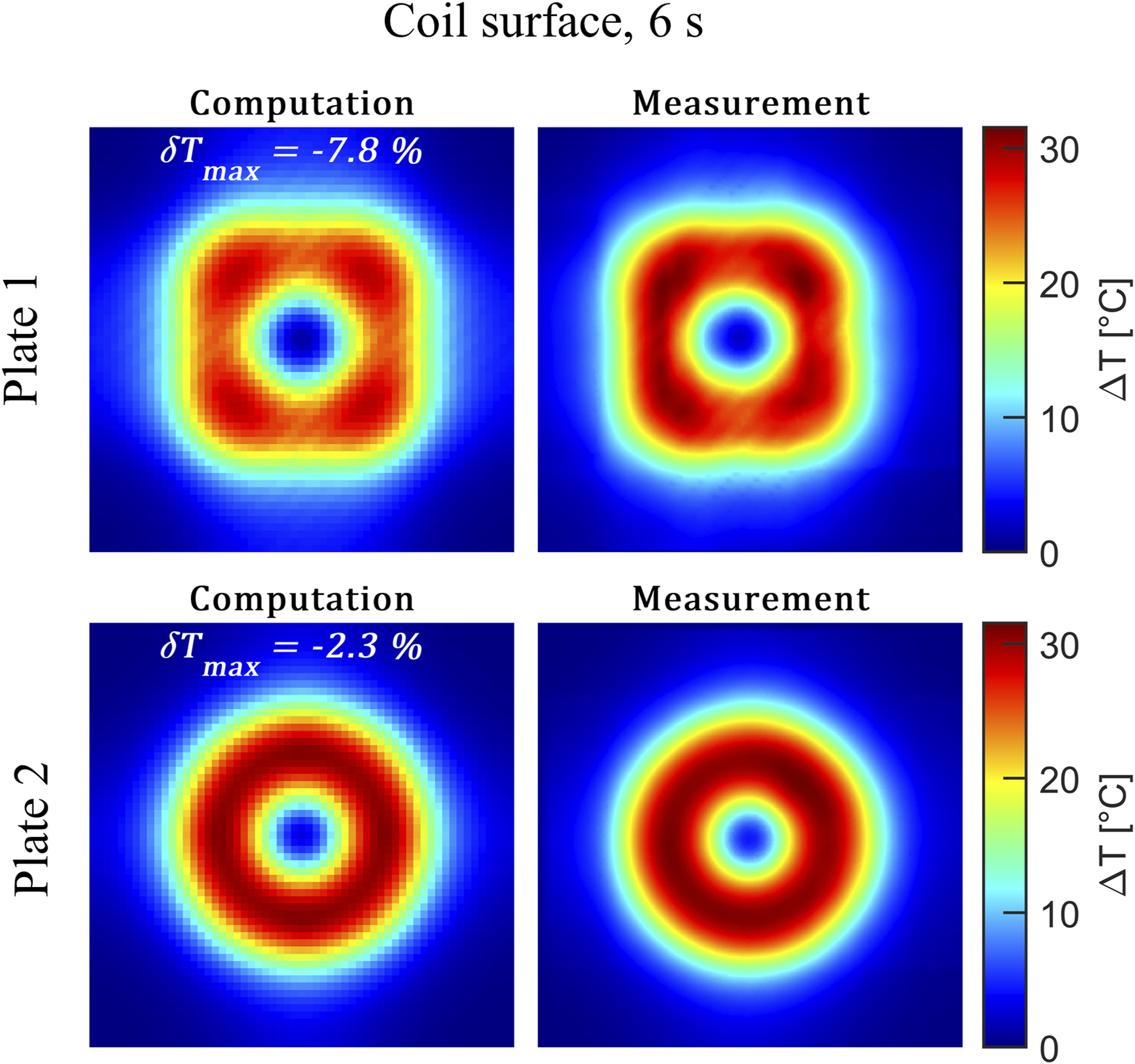
The presented comparisons between simulation and measurement show that the model generates a good prediction of the macroscopic temperature distribution during the temperature increase rates of ΔT _max /t ≈ 7°C/s, similar to the studies by Lundström et al.^12,22 The thermographic measurements only give information about the temperature but indirectly the temperature distribution also can be used to interpret the instantaneous heating power distribution. However, to capture a thermal image of the surface minimally affected by the thermal diffusivity of the material, the image needs to be captured rapidly after the induction heating has started. The thermographic camera captures 30 frames per second and therefore the shortest heating duration that can be evaluated is approximately 0.033 s. To obtain measurable temperature increases during such a short duration the induction power needs to be significantly higher than the induced power of approximately 400 W used in the previous experiments. Figure 23 shows a case when the induced power is adjusted, to be in the upper power range allowed by the equipment (the maximum power is 15 kW), which resulted in the maximum surface temperature increasing rate ΔT _max /t > 400°C/s for plate 1 and ΔT _max /t > 250°C/s for plate 2. The three initial thermographic frames are presented along with the corresponding simulation results. Regarding the maximum detected temperature, the difference between simulation and measurement is noticeable, which however, is not surprising; the thermal model considers homogeneous domains where the power is generated uniformly, and the thermographic measurements are limited to measure the surface temperature and internal hotspots can only be revealed indirectly as the heat diffuses through the thickness. Despite this, the model provides a good prediction of the relative distribution of the power in different tow-directions and where hotspots may be expected during high power input. This detailed tow temperature pattern could not be extracted using the previous presented models by Lundström et al.^12,22 due to the cross-ply representation used in those studies.

Figure 23.

Temperature distribution on the front surface for plate one and plate two at three different timestamps. The images are captured during the heating. The coil current is 190 A for plate 1 and 125 A for plate 2. Using equation (30) the induced power can be calculated; 14.1 kW in plate 1 and 11.5 kW in plate 2.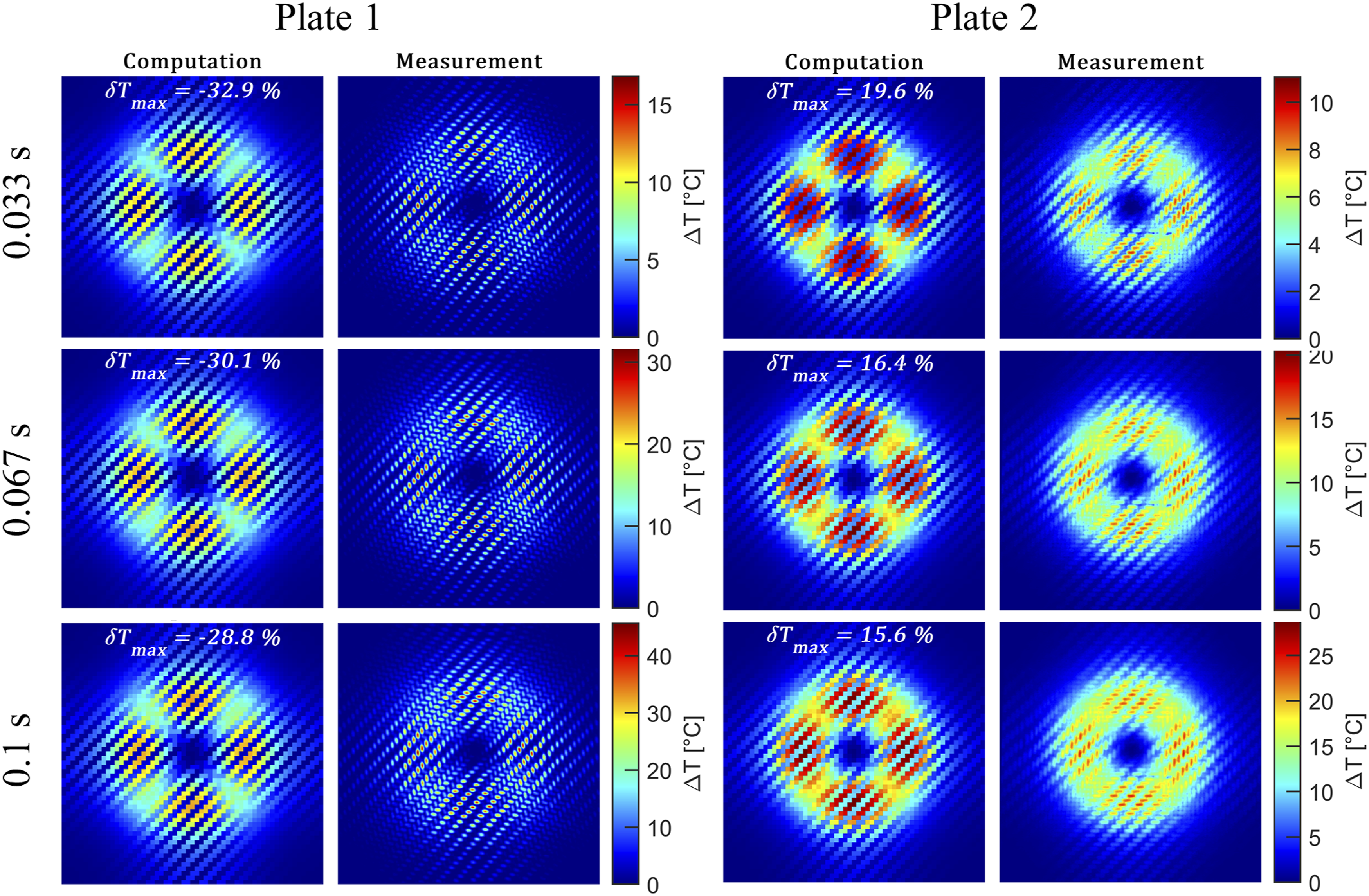

Conclusions

This study shows how induction heating of CFRP can be modelled with a network of discrete resistors by solving a linear equation system based on Kirchhoff’s circuit laws. The temperature distribution is computed using the finite difference method to solve the heat equation. In the thermal part of the model the woven CFRP is discretized into volume elements in which the induction heating power and temperature are uniformly distributed.

It can be concluded, based on the comparison between simulations and measurements, that the model provides a good prediction of the temperature pattern in CFRP during induction heating, especially for CFRP with a high fibre volume fraction (0.67). A woven fabric CFRP is intuitively discretised into a resistor network based on the woven structure and using the electric field from a simple axisymmetric finite element model, the voltages over each resistor element can be extracted. The currents in each ply can be determined separately, without the need for solving Maxwells differential equations in three dimensions. It can be concluded that the inductive characterization of the resistance between tows is valid due to the good agreement between simulated and measured temperature distribution.

To visualize the induced power distribution using thermographic recordings, the influence from the thermal diffusivity needs to be minimized and thus the images must be captured rapidly after initiated induction heating. To maximize the temperature increase per captured image the coil current was maximized to use the frequency inverter in its upper power range, close to 15 kW. The comparison between simulation and measurement, shows that the simulation model provides a good indication of the relative heating power pattern and thus can predict the regions of potential temperature hotspots during high power inputs. Regarding the absolute surface temperature, the difference between simulation and measurement is noticeable which is due to the fact that the significant local temperature gradients induced by the high power during such short time would require a smaller element size to be predicted in detail.

This article presents the case with bidirectional woven fabric, but the model could be modified to handle arbitrary fibre directions. The resistive representation used in this model show good agreement with thermographic measurements, but for higher frequencies it may be necessary to consider a capacitive component. This model can easily be upgraded with temperature dependent properties and capacitive coupling between crossing fibres, if needed.

The presented approach enables prediction of the induced heat distribution on tow size level in a woven CFRP, by using significantly fewer nodes compared to the continuum representation in a three-dimensional finite element model. This model makes it easy to predict current paths and to understand how much of the total heat that is generated within the fibre tows and how much that is generated in the junction between fibre tows, information that is difficult to extract from other models.