Sage Journals: Discover world-class research

Abstract

In this paper a rapid method for residual cure stress analysis from composite manufacturing is presented. The method uses a high-fidelity path-dependent cure kinetics subroutine implemented in ABAQUS to calibrate a linear elastic model. The path-dependent model accounts for the tool-part interaction, forming pressure, and the changing composite modulus during the rubbery phase of matrix curing. Results are used to calculate equivalent lamina-wise coefficients of thermal expansion (CTE) in 3 directions for a linear temperature analysis. The goal is to accurately predict distortions for large complex geometries as rapidly as possible for use in an optimization framework. A carbon-epoxy system is studied. Simple coupons and complex parts are manufactured and measured with a 3 D scanner to compare the manufactured and simulated distortion. Results are presented and the accuracy and limitations of the rapid simulation method are discussed with particular focus on implementation in a numerical optimization framework.

Keywords

Rapid method distortion prediction residual cure stress analysis tool-part interaction thermal expansion carbon-epoxy system

Introduction

Residual stress analysis – Background and state-of-the-art

The modern composites industry is rapidly evolving and manufacturing techniques and processes to produce optimized reinforced polymer composite parts are constantly being refined. Despite this fact, cure induced distortion due to residual stresses is still a major cost and risk driver within composite manufacturing in the aerospace industry in particular.

On the micro-scale, process-induced residual stresses occur primarily due to different behaviour with temperature (T) and degree of cure (DoC) of the resin and the fibre.¹ In thermoset manufacturing processes, the resin is initially a mostly uncured liquid at processing temperatures. One widely used traditional aeronautical composite system consists of carbon fibre reinforcement and epoxy cured at elevated temperatures (often 180°C although other temperatures can be used) in an autoclave. During the manufacturing, the resin undergoes phase changes from a liquid to a solid. These phase changes cause volumetric shrinkage of the resin as it solidifies; also changing its mechanical properties and thermal expansion coefficient in the process. Together with external constraints and influences, like tool-part interaction effects and thermal gradients, it leads to a build-up of internal stresses in the composite part. These stresses in turn causes shape distortions which depend on the level of residual stress and the local stiffness of the component. Distortions can cause delays in production, require late phase re-working of tooling or extensive shimming to compensate for assembly tolerances, cause damage during assembly, and lead to expensive scrappage. For these reasons, avoiding or controlling the distortion in manufacturing is critical to cost control in composite production. Hence, accurate simulation of residual stress induced distortion is vital in order to cost effectively develop and employ methods for compensation, control, and correction of shape distortions. Accurate simulation of these effects will become even more important as unbalanced and non-symmetric layups become of interest for highly weight critical applications.

Over the years several methods have been developed for the purpose of residual stress analysis by assuming either elastic or viscoelastic material behavior of the curing matrix. In an early work, White and Hahn² developed a methodology to predict residual stresses in composites using a viscoelastic approach. Subsequently Zobeiry³ and Prasatya⁴ developed similar methodologies to predict residual stresses taking into account the full viscoelastic behavior of the matrix. Several other notable works have also been performed over the years in regards to the investigation and modelling of process induced deformations (PID) during composite manufacturing processes, including⁵ where a two step finite element (FE) model is developed to predict spring-in of C-sections, where assumptions are made in which the material is assumed fully relaxed until the vitrification point of the resin. The subsequent FE model is composed of two steps, where calculations are performed before and after the said vitrification point. In another work by Tsukada et al.⁶ a novel method involving the use of fiber Bragg grating sensors to measure the PID strains that developed during the processing of thick thermoplastic composite parts was described. Moreover, in,⁷ a comprehensive experimental investigation of the effects of cure cycle, tool-part interaction, geometry and layup on the spring-in behaviour of autoclave processed composite parts was performed.

However, in previous studies,^2,4,8 linear viscoelasticity is assumed while developing the necessary constitutive models. While there exists other works that assume non-linear viscoelasticity, it is much more complicated and the available literature suggests that a linear viscoelastic approach is sufficient to model curing induced residual stresses,^9,10 since the strains developed during processing are thought to be infinitesimally small. Regardless, a full viscoelastic implementation, linear or otherwise, is currently not feasible for industrial applications due to the extensive material characterization and computational costs required.

One of the most frequently used approaches in use today is the Cure Hardening Instantaneously Linear Elastic (CHILE) model.^3,11 In this model the properties are assumed to change during curing, depending on temperature and cure with the material response assumed to be elastic at each time instant. Under certain conditions like in a simple one-hold curing cycle, both spring-in angles and warpage can be predicted for a composite part reasonably accurately using this approach. This approach has been implemented e.g. in the commercial software COMPRO by Convergent.

In their work, a simplified approach was proposed by Svanberg and Holmberg¹² in the form of a path-dependent model (as opposed to rate dependency) based on the incrementally written differential form of viscoelastic relaxation formulated by Zocher et al.¹³ The proposed method was a pseudo-viscoelastic formulation which is an improved form of the CHILE model taking elements of viscoelasticity into account. The path-dependent model can predict residual stresses and shape distortions relatively accurately and is robust in nature due to its ability to handle complex curing cycles. It has been implemented in various commercial tools for process simulations (PAMDISTORTION and LUSAS HPM) of industrial relevance. Several different works^9,10,14 have implemented the path-dependent model in various commercial softwares for simulating manufacturing processes ranging from RTM to prepreg layup and concluding reasonable accuracy of the model for the stated purposes. In fact, recent reviews¹⁵ have pointed out that the CHILE model and the path-dependent models are the most widely used models for the computation of residual stresses currently for various applications.

Modelling of residual stress distortion using numerical methods is yet to reach its full potential despite the tools mentioned above being commercially available for some time. Areas for improvement include prediction accuracy and computational time, which are the points that will be mainly considered as within the scope of this work especially for the purpose of prototyping.

Recently, new studies have emerged^16–19 that have proposed an improvement to the path-dependent model taking into account thermorheologically complex materials and also the dependency of the glassy and rubbery stiffnesses on temperature. For the work conducted within this paper, these improvements have been added to the existing path-dependent model and subsequent analyses for the high-fidelity FE modelling.

Improvements to the path-dependent model

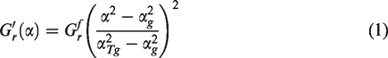
The path-dependent model proposed by Svanberg and Holmberg¹² assumes that the rubbery modulus is independent of the degree of cure. In Saseendran et al.,¹⁸ it has been determined through dynamic mechanical and thermal analyses (DMTA) on neat resins that this is not true. There is evidence to support that the rubbery modulus of an epoxy resin (Huntsman LY5052) exhibits a marked dependence on the degree of cure. Moreover in earlier works, notably by Adolf and Martin²⁰ have also determined this to be true. In their work, Adolf and Martin described the dependence of the rubbery shear modulus $G_{r}^{'}$ on the degree of cure α using the relationship

G_{r}^{'} (α) = G_{r}^{f} {(\frac{α^{2} - α_{g}^{2}}{α_{T g}^{2} - α_{g}^{2}})}^{2}

(1)

where

G_{r}^{f}

is the fully cured rubbery shear modulus, α_g is the degree of cure at gelation and α_Tg is defined as the degree of cure attained for curing at various temperatures such that the material is in glassy state at the end of the curing cycle. A comparison of Eq.1 with experimental results is shown in Figure 1. However, Mours and Winters²² have argued that the models developed by Adolf and Martin are applicable only for systems with low molecular weight as high molecular weight systems did not tend to provide unique master curves. This argument was also confirmed experimentally by Mours and Winters.²³ Another study by Emri²⁴ also agrees with the observation by Mours and Winters, arguing that high molecular weight systems show non-linear dependence of the shift factors on the response time. But for all practical purposes, most of the commercially available epoxy systems can be classified as relatively low to medium molecular weight systems. However, it is also to be noted that the molecular weights epoxy systems used in some aerospace applications range from medium to high due to the presence of additives, due to the processing conditions that may be required. Prior DMTA tests on the epoxy system under consideration indicate that it is indeed thermo-rheologically simple and hence it was concluded that this model dictating the dependence of the rubbery modulus on the degree of cure is applicable to the system under consideration.

Study objectives

The current study has four objectives. First, to introduce the modification presented in the previous section to the existing model as described by Svanberg and implement this in an FE code. Secondly, to use this improved path-dependent model to develop a rapid methodology to predict distortions of moderately less accuracy significantly faster. Thirdly, validate the method on the coupon level using simple geometry. Finally, to validate the method on a complicated part with double curvature.

Development of the rapid methodology is explained in the next section. The following sections present a validation of the rapid method comparing simulation results to the path dependent method and experiments. This is first performed at the coupon level, then the component level. The paper is then concluded with discussion and observed outcomes.

The rapid methodology

The methods described above are well known and accepted for process simulation of composites in the aerospace industry. While accurate, none of these approaches are well suited for optimization with large models including many design variables due to long computational times. Herein lies the motivation for the rapid methodology proposed in this paper.

The aim of the rapid method is not to predict distortions to the same level of accuracy as the high-fidelity model, but rather to create a fast and efficient way of predicting the most important deformation modes for a complex component accurately enough, so that pro-active design exploration can be performed early on in the design process.

Figure 1.

The dependency of the rubbery modulus of an epoxy resin with degree of cure.¹⁸

The basis of the rapid method is the use of a set of artificial coefficients of thermal expansions (CTEs) on the ply level, that will replicate the distortions calculated using a full cure analysis. Here, a full cure analysis means using the improved path-dependent model described in “Improvements to the path-dependent model” section, in addition to accounting for the effects of tool-part interaction and forming forces for an arbitrary material and cure cycle. The artificial CTEs are calculated using specific reference/calibration geometries explained below. Since these values are calculated based on the full cure model output, they account for both thermal and chemical shrinkage. As these CTEs are assumed to be ply properties, they can then be used as input to calculate shape distortions for an arbitrary FE model using a simple linear temperature load, regardless of geometry. The method requires a mesh using solid elements, or continuum solid elements. The three main steps in the method are summarized in Figure 2, and explained in more detail below.

Figure 2.

A summary of the rapid method.

Step A

In the first step, the distortion of two reference geometries are calculated using the path-dependent cure model originally developed within,²⁵ including improvements proposed in Saseendran et al.^18,19 as described in “Improvements to the path-dependent model” section to account for the change in modulus during the rubbery and glassy state during cure. These models are implemented in Fortran subroutines for ABAQUS.

In order to perform these simulations (as with any cure kinetics model) a significant amount of input data is needed. In this case, a testing campaign to define the matrix material has been performed including differential scanning calorimetry (DSC), CTE measurements of the neat resin, glassy state material testing of the neat resin, and dynamic mechanical thermal analysis (DMTA). In addition, an experimental campaign similar to Twigg et al.²⁶ was performed to evaluate the tool-part interaction behaviour and validate input data for the model.

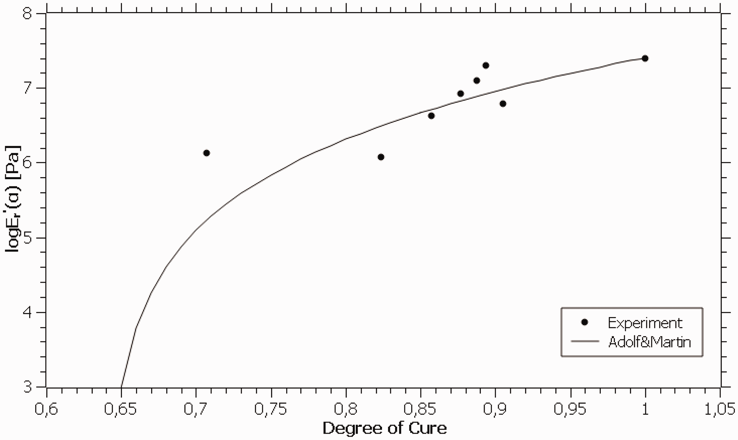
The two calibration geometries, an L-profile and a flat plate are used. The geometries are selected to minimize the coupling effects between CTE-22 and CTE-33, see Figure 3. A long, slender, flat plate with a cross ply layup $[0_{4}, 90_{4}]$ is used to maximise the out of plane warpage and isolate the effect of CTE-22. A quasi-isotropic layup is used in an L-profile to minimise the in-plane thermal strains, and maximise the effect of out of plane deformations due to chemical and thermal matrix shrinkage, isolating CTE-33. The CTE in the fibre direction (CTE-11) is set to the measured value and kept constant throughout steps A-C.

Figure 3.

The two reference geometries and layups used in the rapid method to calculate the artificial CTEs.

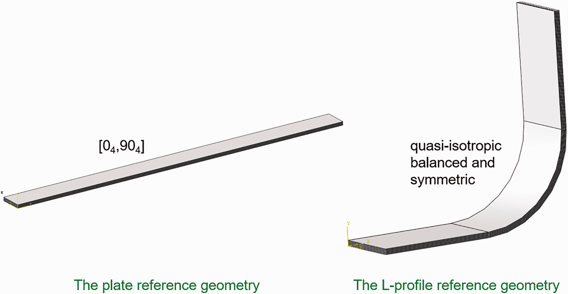
For both reference geometries, the full cure simulations are done to simulate the tool-part-interaction, and the pressure from the bag during the curing phase, see Figure 4. De-moulding of the component is simulated by removing the tool and the bag pressure from the model and allowing the final deformation to be achieved isostatically, see Figure 5.

Figure 4.

A more detailed illustration of BC1 and BC2 together with the pressure part of LC1. The label by the constrained nodes in BC2 indicate the constrained DOFs.

Figure 5.

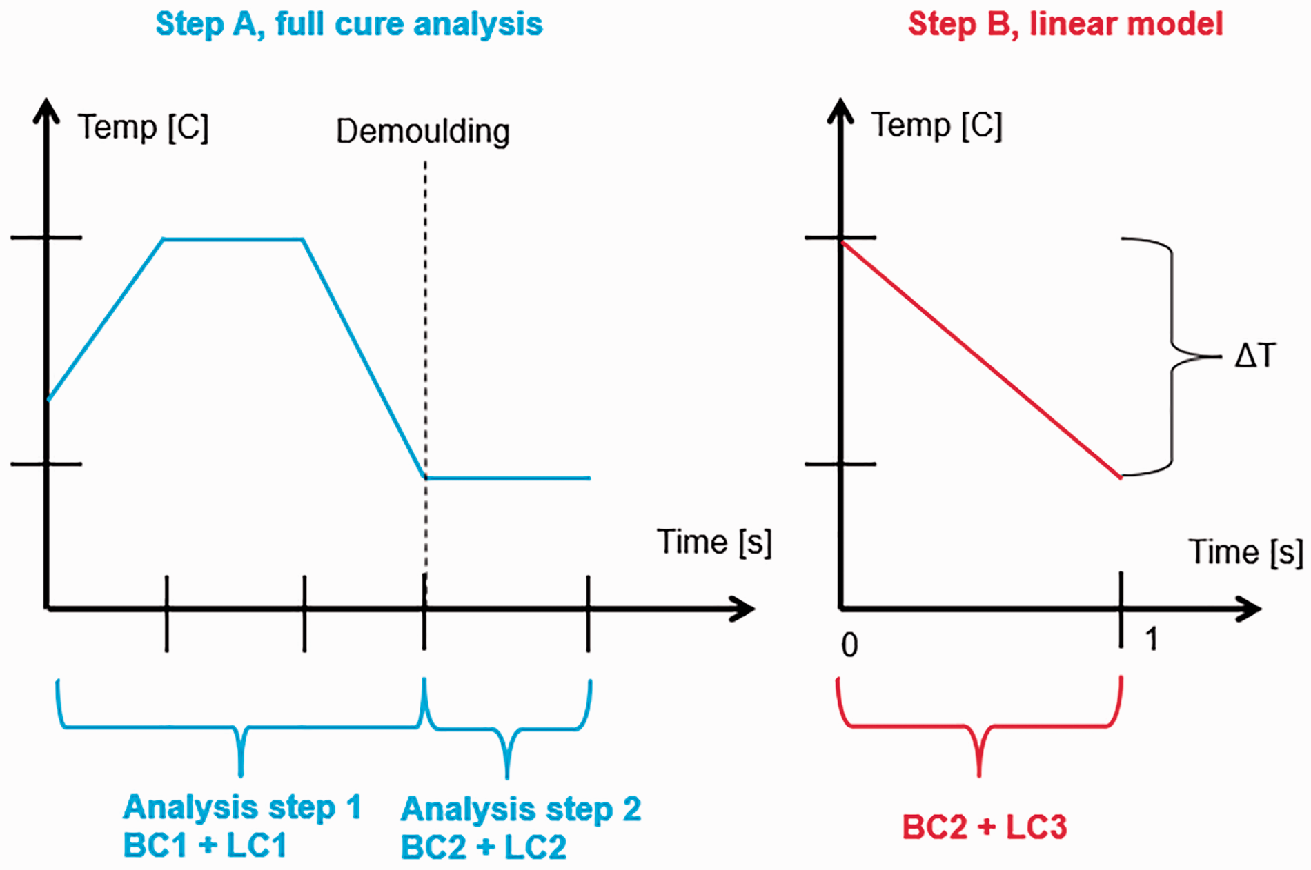
Illustration of when the two boundary conditions and three load cases are active. Note that the full cure analysis is performed in two steps.

Two analysis steps are used in Step A to allow the boundary conditions to change after the cure cycle is completed and the part is de-moulded. During the cure cycle (analysis step 1) the boundary condition BC1 and load case LC1 are used while BC2 and LC2 are used during de-moulding in analysis step 2, see the left figure in Figure 5. The loads and boundary conditions can be described as follows.

BC1: One corner of the tool is locked in all degrees of freedom (DOF). Symmetry is applied to four sides to prevent rigid body motion and allow tool expansion, see Figure 4.

LC1: A temperature field corresponding to the cure cycle is applied on the bag side surface of the part and all external tool surfaces not under the laminate. The tool is assumed to be heated via conduction from its surface, and not to have internal heating elements. A pressure load corresponding to the equivalent pressure from the vacuum bag is applied on the bag-side of the part, and a contact condition to allow in-plane slip with friction is applied between the part and the tool. Inter-laminar slip is not permitted within the model for the laminate. Figure 4 shows these conditions.

BC2: In the second analysis step the part is de-moulded, i.e. constraints imposed in BC1 are removed and isostatic boundary conditions are enforced as shown in Figure 4. This eliminates rigid body motion and allows the part to achieve its equilibrium state.

LC2: Pressure is removed from the bag-side and the temperature on the bag-side and tool-side surfaces are set to ambient.

The resulting deformation of one node per calibration model are extracted. This point, denoted P, is located on the opposing edge from the boundary condition and in the mid-plane of the composite, see Figure 6. The direction of displacements are also in indicated Figure 6.

Figure 6.

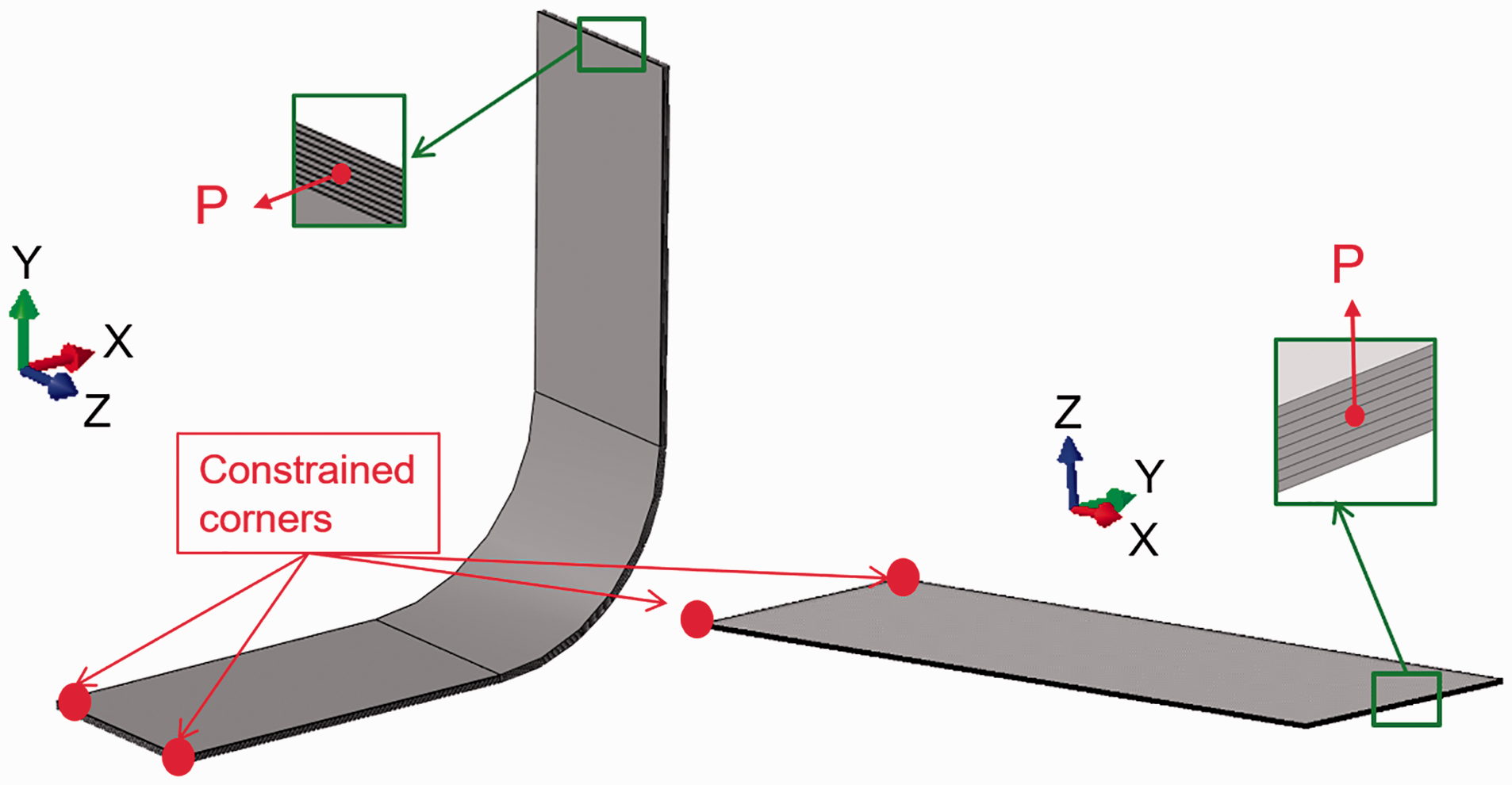
The location of point P in the plate and L-shaped models.The arrows indicate the direction of the extracted displacement result.

Step B

Once the full cure analysis has been carried out, the artificial CTE-values can be calculated. This is done iteratively by altering the values of CTE-22 and CTE-33 in two linear models of the same plate and L-profile used in the full path-dependant simulations. A python script is used to automate this process.

The plate and L-profile mesh from Step A can preferably be used also in Step B, removing the tool from the model. A linear load case LC3 is introduced, corresponding to a temperature drop equivalent to the largest difference in temperature during the cure cycle, here denoted ΔT. See the right hand side of Figure 5 for clarification. The boundary conditions (BC2) and points to extract nodal displacements used are the same as in the second analysis step of Step A.

The values of CTE-22 and CTE-33 for a single UD ply are iteratively adjusted using the python script until distortion in the linear simulation matches that of the path-dependent simulation. Absolute convergence is not always possible, so a tolerance is specified by the user. The result of this process is the values of CTEs that yields the closest match in deformation.

Step C

The artificial CTE-values from Step B are assumed to be ply properties of the specific material system used in step A and B. The resulting artificial CTE-values can then be used for shape distortion simulations of an arbitrary geometry.

A limitation of this statement is of course that the cure-cycle, constituent materials and mould surface treatment remain constant throughout the analysis and design process. An alteration to any of these aspects constitutes a change to the problem at its foundation, and the entire process must be repeated. Mould geometry is however not as intrinsically coupled to the problem as these three aspects. While no theoretical proof can be detailed showing why the rapid method can be used for an arbitrary geometry, the authors believe that the correlation between simulations and relatively complex geometry provided herein, provide sufficient empirical evidence that the rapid method is valid.

Coupon level validation

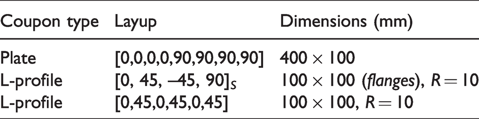
To provide a basis for validation and comparison of the two numerical methods, a number of coupons, see Table 1, were manufactured and the distorted geometries were measured with a GOM Atos 3 D laser scanning system.

Table 1.

Coupons analysed in the current paper.

Coupon type	Layup	Dimensions (mm)
Plate	[0,0,0,0,90,90,90,90]	400 × 100
L-profile	[0, 45, –45, 90] _S	100 × 100 (flanges), R = 10
L-profile	[0,45,0,45,0,45]	100 × 100, R = 10

In the current paper, the manufacturing method was vacuum infusion and oven curing at elevated temperature. Carbon-Fibre non-crimp fabrics and uni-weave materials were used together with a single component epoxy system. Details of the fabrics and epoxy system are not included due to confidentiality.

Simulation results and comparisons to manufactured geometries are provided below.

Crossply plate

Figure 7 shows the predicted distortions for the full path-dependent method (Top), the rapid model (Middle), and the result of a 3 D scan of a manufactured specimen (Bottom). Distortion in the FE model is given in a local coordinate system defined by a plane through the two ends of the specimen, comparable to measuring vertical displacement from a table top where a specimen would rest on its ends. For the path-dependent model, the maximum distortion is calculated as 28.25 mm, and for the rapid method, 27.75 mm. For the measurement, the maximum distortion is given as 27.45 mm. Clearly, both models give a very good representation of the distortion trend, and magnitude.

Figure 7.

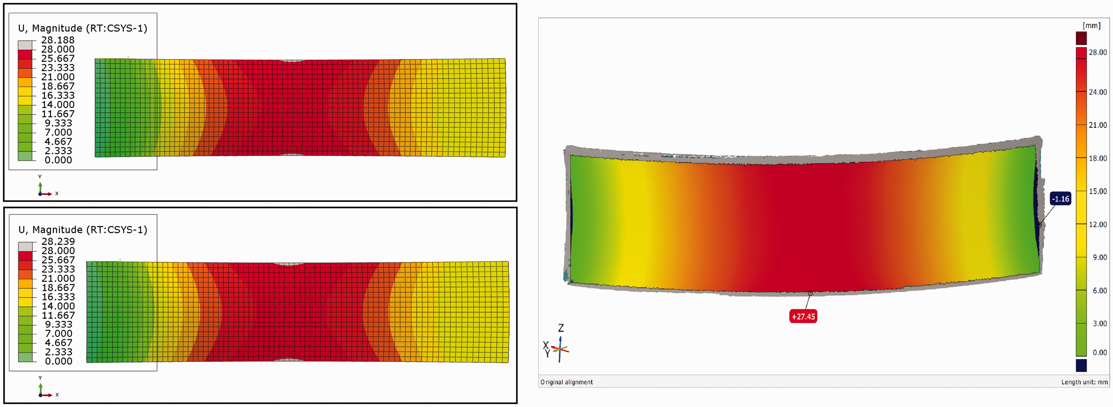
Simulated distortions in cross-ply laminate for path-dependent model (top) and rapid method (middle) compared with measured distortions (bottom).

L-Profiles

Distortion of the Quasi-isotropic L-profile for the path-dependent and rapid model are shown to the left and right respectively in Figure 8. The displacement shown is of one flange in the x direction, i.e. the spring-in distance. As can be seen, the two results show very good agreement with each other, differing only on the order of 0.04 mm. Figure 9 shows the results for the simulations of the unbalanced L-profile. The path-dependent model is to the left, and the rapid model to the right. As seen in the figure, the rapid model captures the twisting of the flange seen in the path-dependent model. The magnitude of predicted distortion is approximately 0.3 mm less.

Figure 8.

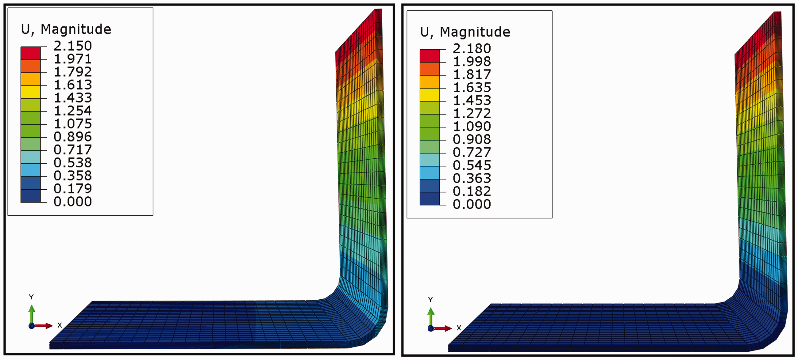
Distortion prediction for symmetric L-profile laminate for path-dependent model (left) and rapid method (right).

Figure 9.

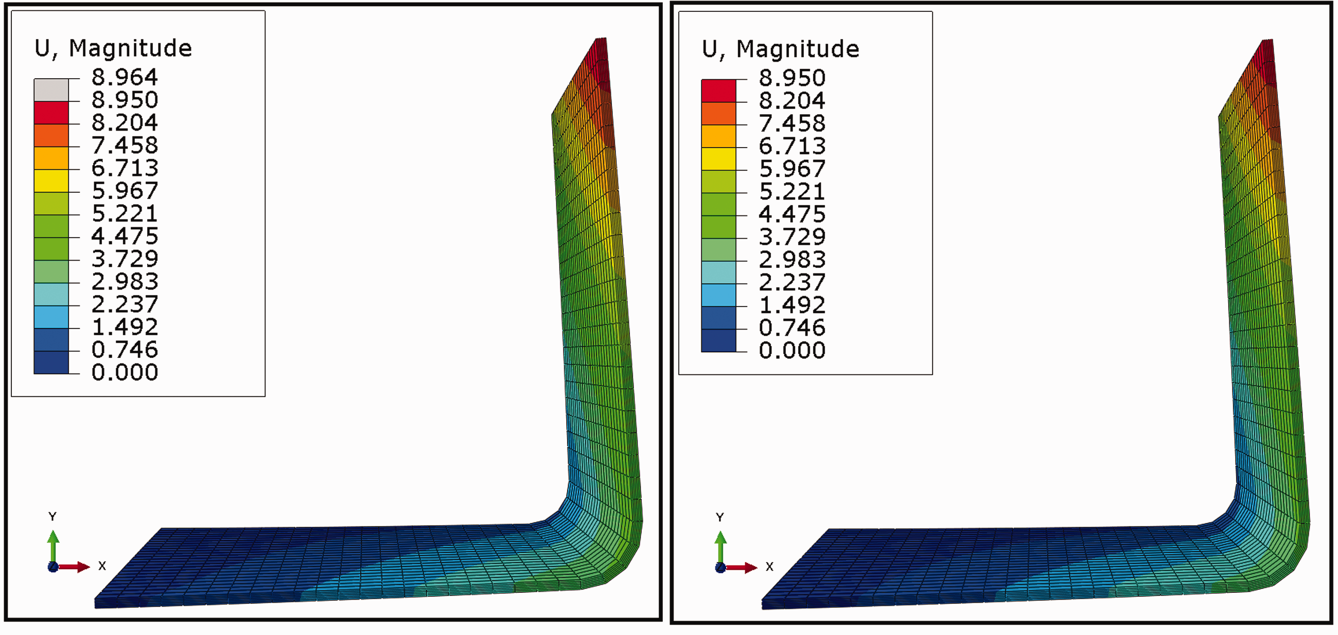
Distortion prediction of un-balanced L-profile for path-dependent model (left) and rapid method (right).

Spring-in angle was chosen as a method of comparing the distortion shown in Figures 8 and 9 with those measured on manufactured parts. Parts were scanned and the angle between tool-side surfaces at 3 different sections along the length of the profile were measured using GOM Correlate software, see Figure 10. The distorted nodal coordinates from the simulation results were exported in a format compatible with GOM Correlate, and the exact same measurements were performed. A comparison of the measured angles from manufacture, and simulation is given below in Table 2.

Figure 10.

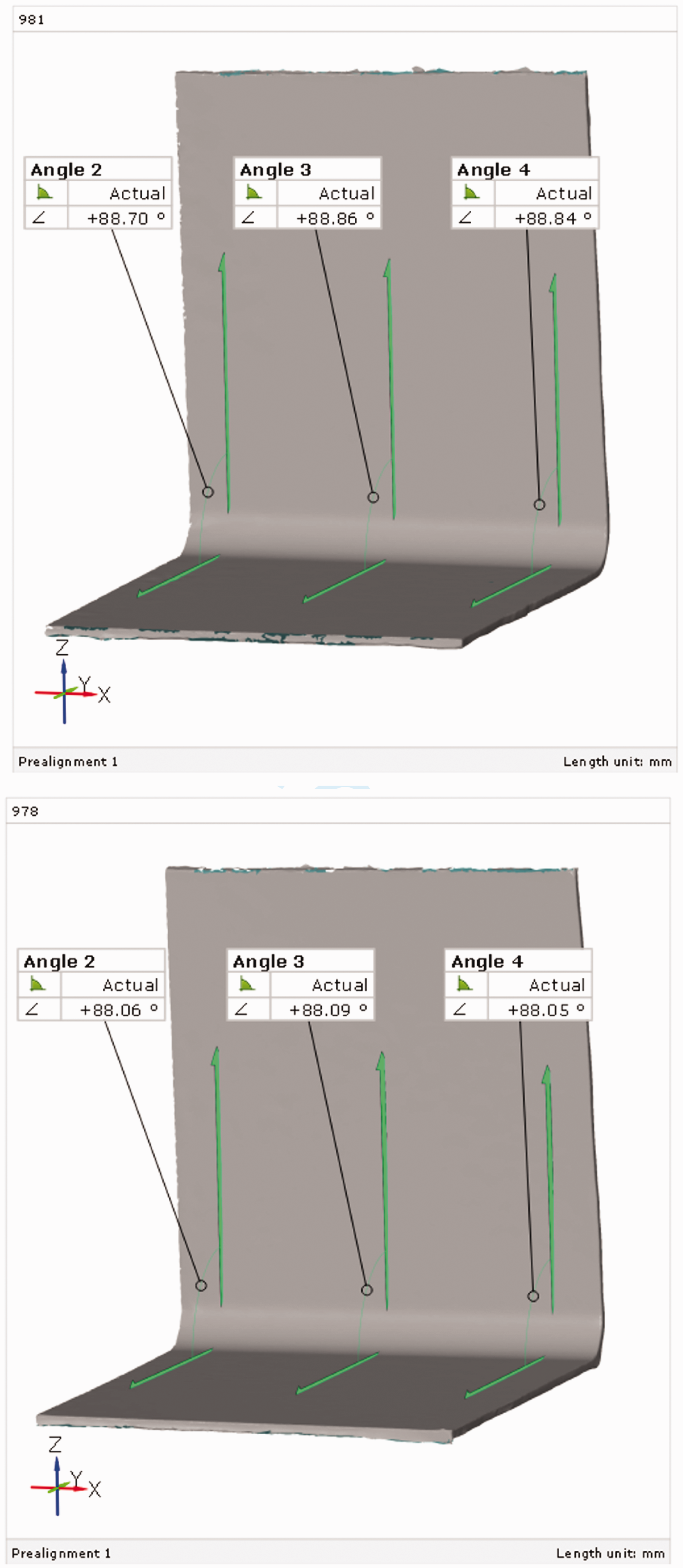
Angle measurements for L-profile, Quasi-isotropic profile (top), un-balanced profile (bottom).

Table 2.

Spring-in angles for L-profiles, experimental and simulated.

		Unbalanced			Balanced
		[0, 90]₄			[0, 45, −45, 90] _s
	Sample	Angle	Angle	Angle	Angle	Angle	Angle	Sample
		1	2	3	1	2	3
Exp.	A	1.91	1.91	1.95	1.03	0.97	1.01	C
	B	1.94	1.96	2.00	1.21	1.14	1.17	D
Sim.	Rapid	1.67	1.71	1.66	1.16	1.16	1.16
	Path-dep	1.82	1.92	1.77	1.06	1.07	1.06

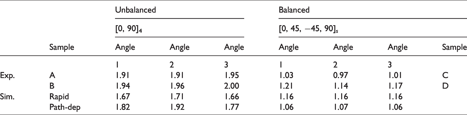
From the data in Table 2, there is both good agreement, and some small discrepancies worth discussing. For reference, samples A and C were manufactured simultaneously on the same tool seperated by approximately 1 cm, as were samples B and D. This was done to ensure the respective sets of samples were subjected to effectively identical cure cycles and eliminate any chances of curing irregularities causing differences between the sample sets. In other words, by manufacturing one of each layup at the same time, potential irregularities in cure would manifest themselves in both samples, and would not introduce false differences between layup types. For the unbalanced layup, the differences between measured angles was less than 0.05°. For the balanced layup, the differences were slightly larger than 0.15°. While this is a very small numerical value, it represents a significant percentage of the spring-in angle. It is interesting to note that the variation between the balanced samples, i.e. the layup traditionally chosen to avoid spring-in distortion, shows more variability than the unbalanced layup. Also, despite being manufactured to the same protocol, it can be seen that the first samples to be manufactured have a slightly lower spring-in angle than the second samples to be manufactured. As only 2 specimens of each were made, it is not possible to draw any statistically based conclusions, but again, the manufacturing results point to a high degree of variability within the material systems, which manifest themselves even for very simple geometries. From the simulation perspective, for the unbalanced profile, both methods clearly predict distortion of the correct magnitude, however they both slightly under predict the spring-in angle. They also slightly over predict the variation in angle due to the unbalance in the layup. For the balanced layup, both methods are self-consistent, and lie within the span of variability from the manufactured components.

Component level validation

To evaluate the method properly, a more complicated part geometry is necessary. A curved Z–profile is used to incorporate male and female radii and double curvature. The part is approximately 500 mm long, 100 mm high and 175 mm wide, and has a nominal theoretical thickness of 3.54 mm. The lower flange varies in length along the part. The part was made of a constant thickness with the layup ${[0, 90, \pm 45, 0_{2}, 45]}_{S}$ .

Two components were manufactured for comparison against model results. A picture of one of the specimens can be seen in Figure 11 together with a blanket plot displaying the thickness variation of the entire part.

Figure 11.

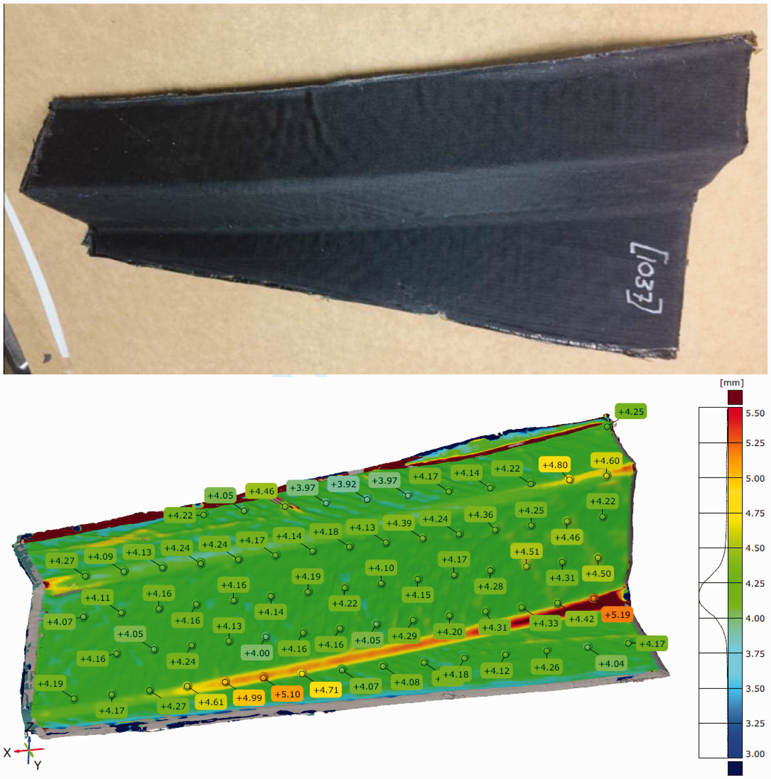
An as-manufactured Z-profile (above) and the global thickness measurement from laser scanning.

For this work, a single layer of elements is used for each layer of material. In total 14 layers were used. Figure 12 shows the FE geometry of the part as seen on the tool (left) with a close-up of the laminate thickness to the right.

Figure 12.

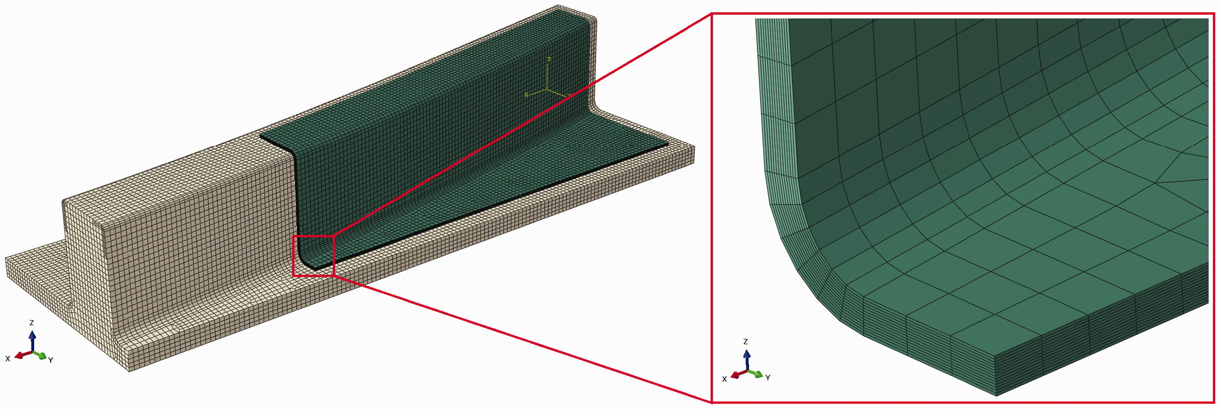
Geometry of the Z-profile and tool (left), and close-up of laminate thickness (right).

Nominal fibre orientation only is used for the models. Effects of the draping process, i.e. fibre misalignment, shearing in the NCFs, wrinkling, etc. are ignored.

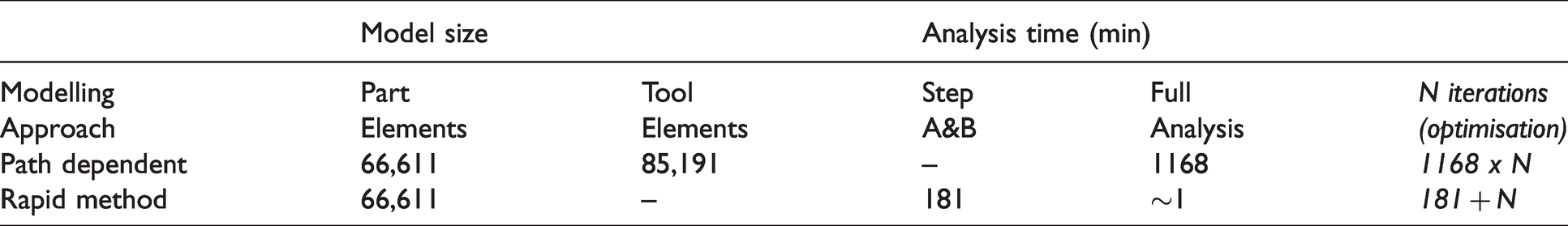
A comparison of the model size and simulation time between the path-dependant and the rapid model is presented in Table 3. Inspecting the data in the table, the question of what effect removal of the tool geometry and tool-part contact interactions has on computational time needs to be addressed. Without question, the addition of a large number of (linear elastic) elements and contact conditions adds complexity and computational time to the model. This is not however the primary driver of computational time. During the full analysis, fortran subroutines are used to calculate the material state (degree of cure) at each temperature increment within the cure cycle. Small steps in temperature are required to maintain stability in the numerical solution, resulting in hundreds (or thousands) of calculation steps depending on the cure cycle and dwell times. Once the thermal solution is finished, the results must be translated from the heat generation analysis output to be compatible as input to the structural analysis problem. This is also done with Fortran subroutines implemented in ABAQUS. Finally, the structural model is also run, where the material properties are calculated at each temperature increment based on the degree of cure at that point, and the effects of changing CTE, chemical shrinkage, changing stiffness, etc are accounted for in addition to the contact conditions. Thus, the path dependent model takes considerably longer to run regardless of tool geometry or contact conditions.

Table 3.

Validation Z–profile model data.

	Model size		Analysis time (min)
Modelling	Part	Tool	Step	Full	N iterations
Approach	Elements	Elements	A&B	Analysis	(optimisation)
Path dependent	66,611	85,191	–	1168	1168 x N
Rapid method	66,611	–	181	∼1	181 + N

The distortion predicted using both methods is given in Figure 13. It can be seen that both models capture the same general distortion behaviour. The rapid model does however appear to slightly overestimate the distortion.

Figure 13.

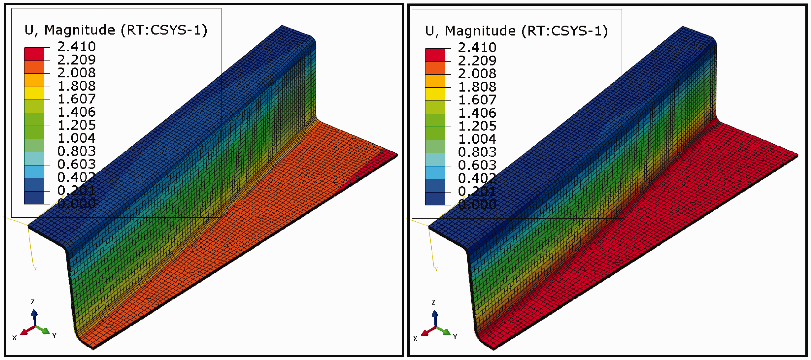
A comparison of the path-dependent (left) and rapid method (right) for distortion of a curved Z-profile.

Comparisons with 2 manufactured components is again performed using laser surface scans and the GOM inspect software. In addition, the spring-in angles formed by the upper flange and the web, and the lower flange and the web at several different points along the length of the profile are measured and compared for both the manufactured samples and the simulation results as performed on the coupons.

Figure 14 shows colour blanket plots comparing deviation between the tool-side surfaces of one of the manufactured components and the simulations. The path-dependent model v/s manufactured is shown to the left, and the rapid model vs manufactured to the right.

Figure 14.

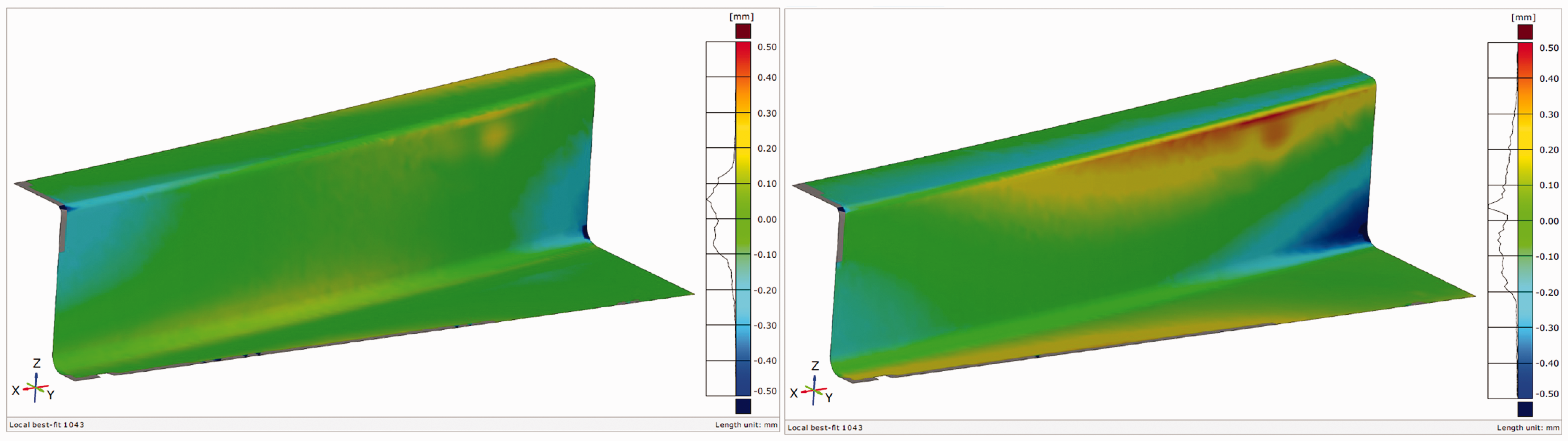
Comparison of the path-dependent (left) and rapid method (right) for distortion of a curved Z-profile with measured component.

The visualisations show a good general agreement between simulation and experiment for a relatively complex geometry. As expected, the path-dependent model shows better agreement. The distribution of deviation between points on the surfaces is visible on the vertical legend. The majority of deviation is within $\pm 0.25 mm$ of the manufactured specimens. Areas where it appears challenging to match the manufactured distortion is along the upper male radius running the length of the profile, and in the corners of the female radius running along the length of the profile. This corresponds well to the most challenging areas to achieve good draping behaviour in manufacture.

Angle measurements of the two experimental samples as well as the simulation results were also performed. The angles were measured at the locations indicated in Figure 15 (left). These locations are offset planes parallel to a vertical plane aligned with the right edges of the profile. The angles are numbered 1-10 as shown in Figure 15 (right). Angles 2 and 4, i.e. the leftmost angles on the lower flange, were challenging to measure, and their values are questionable. This is due to the high local curvature of the section in that area. The best fit straight line at the corner is a poor approximation. For this reason, the values of angle 2 and 4 should only be considered as a reference, and not given equal weight in the evaluation.

Figure 15.

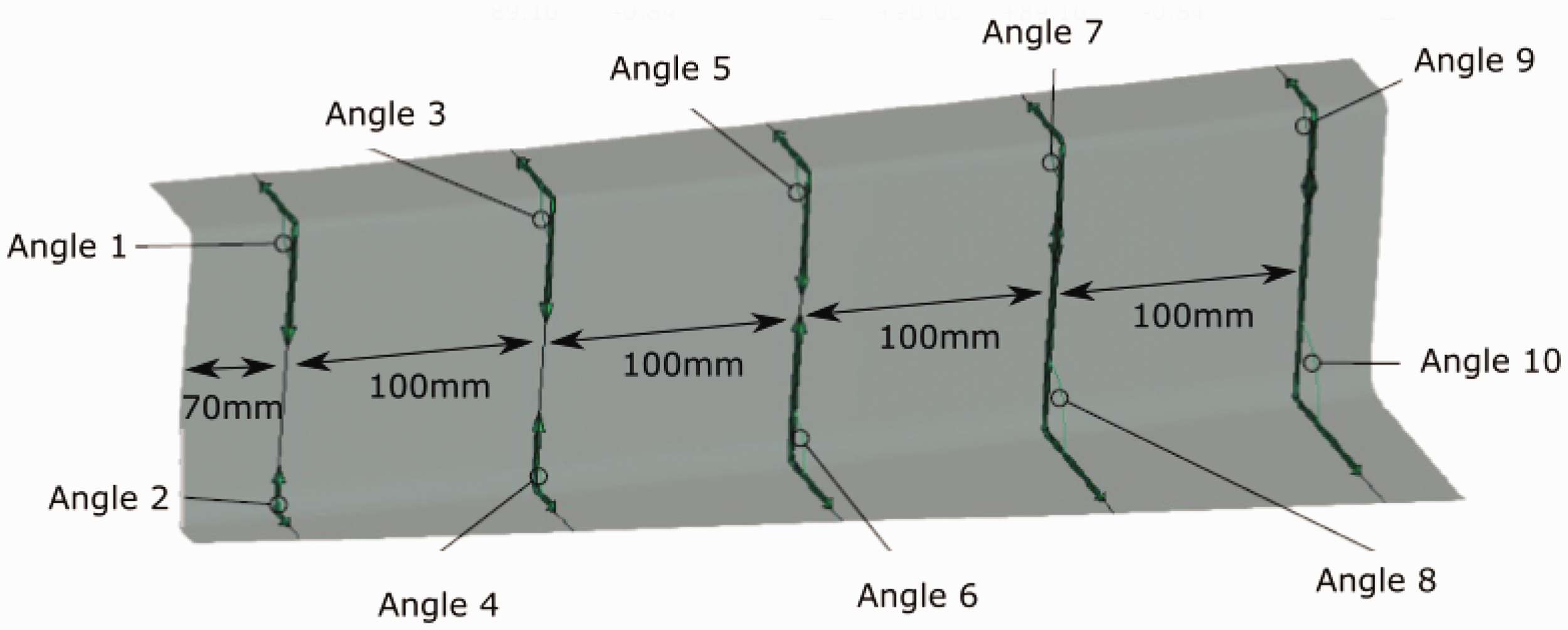
Location of measurement points for profile angles (left), Location and names of angles measured on profiles (right).

Spring in angles for the simulation results and the experimental measurements are visualised in Figure 16. In the left of the figure, five points along the length of the top flange (corresponding to angle 1,3,5,7,9 in Figure 15) are directly comparable between manufactured and simulated components. For reference, four extra points are included for the manufactured part along the same flange in between the numbered angles. In the right of the figure, four points along the bottom flange (corresponding to angle 4,6,8,10 in Figure 15) are directly comparable between the manufactured and simulated parts. Additional points are included for the manufactured specimen. Angle 2 for the simulated results has been omitted from the figure. This was done because the high degree of local curvature on the simulated surface proved effectively impossible to find a “best fit” straight line through the cross-section. This was not as problematic for the manufactured specimen, because the resulting flange was slightly longer than the nominal design.

Figure 16.

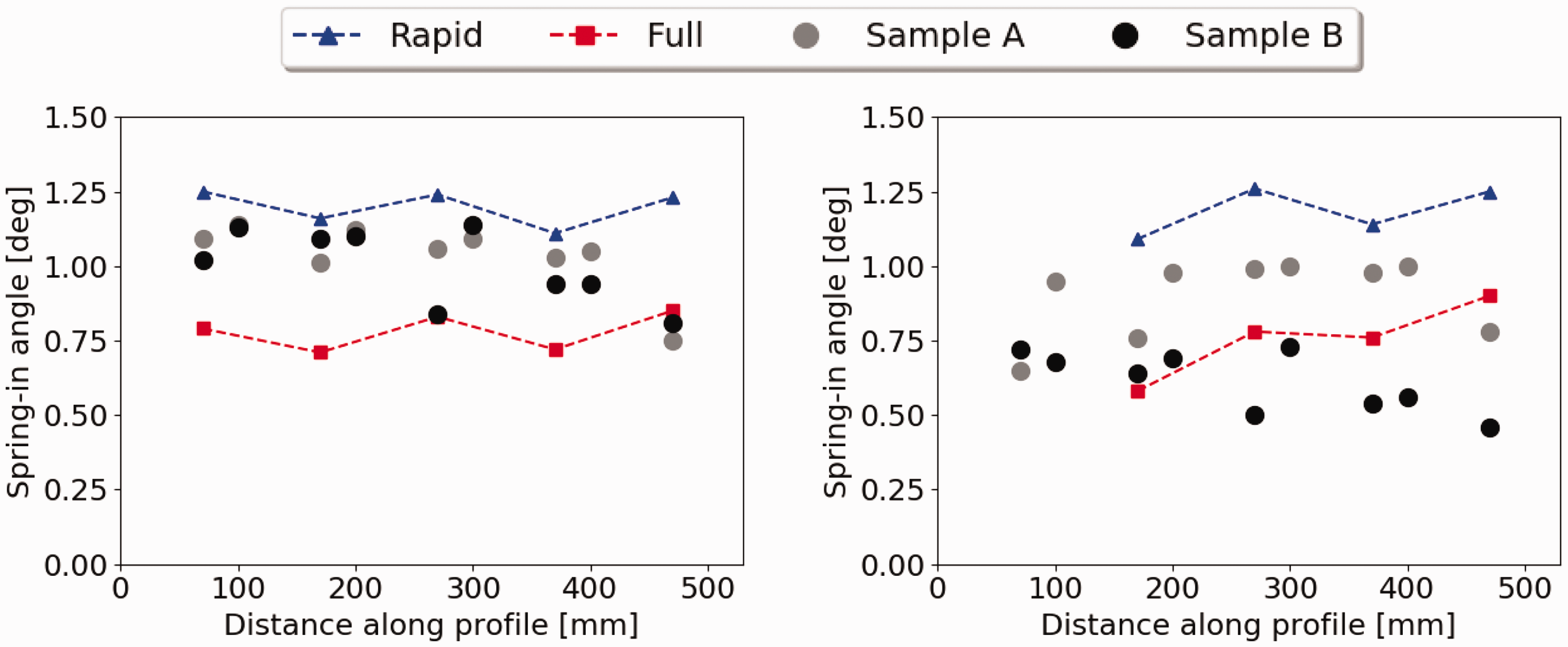
Spring-in angle measured along the length of the upper (Left) and lower (Right) flange for manufactured and simulated profiles.

Overall, the data in Figure 16 gives a very clear picture of the accuracy of the simulation methods, and the variation in spring-in angle for the manufactured specimens. For both the upper and lower flange, the rapid method appears to overestimate the spring in angle. The path-dependent model appears to underestimates the angle for the top flange, but be somewhere in the middle of experimental variation for the bottom flange. In general, the magnitude of over and under estimation of the spring-in angle is similar to the variation in angle seen between specimens.

Discussion

The results presented in the previous two sections gives a clear picture of the potential for the rapid method proposed in this paper.

From the outset, the goal of the work was to develop a method for cure distortion simulation that could be implemented in an optimization framework. This implies that the method should be accurate enough to capture the fundamental physical modes of distortion and to do so at a fraction of the computational time compared with a state-of-the-art model. Judging from the good agreement between simulations and measurements for both the coupon specimens and the more complicated z-profile, this has been achieved.

Despite being state-of-the-art, the path-dependent model is not capable of capturing the exact distortion of the large z-profile manufactured and described in this work. While there are likely further improvements that can be made, the method nevertheless does a very good job of predicting distortion in a complicated part with a challenging manufacturing process. On a global level, the distorted surfaces are within 0.2 mm of experiment for most of the surfaces. This accuracy is despite the fact that the model does not incorporate any of the manufacturing process induced sources of distortions e.g. fibre bridging in the female radius, fibre angle deviation from nominal, shearing or wrinkling of the NCF in compression or tension along the flanges. These most certainly occur to some degree indicated by the high level of variation in the spring in angles. It is also worth mentioning that the process studied here is out-of-autoclave vacuum infusion (where plies of NCF materials must be held in place on the tool while vacuum is achieved) as opposed to much work in the literature focusing on pre-preg carbon laminates.

Measurement of the so called ‘spring-in’ angles are also potential source of uncertainty. Spring-in angles are often referred to in composite manufacturing, however exactly how they should or can be measured is not obvious. For the present case, the local curvature and warping of the short and relatively thick flange meant measuring these angles was nearly meaningless for angle 2 and 4. For the other longer, relatively flatter sections of flange, it appears to work much better.

Another promising aspect can be seen when comparing simulations and measurement. The rapid method appears to consistently overestimate spring-in while the path-dependent model underestimates it. Should this tendency prove to be consistent for other geometries, it would be an excellent tool in the early design phase. An optimization can be performed using the rapid method, where distortions are” amplified”, and a validation simulation can be performed for a one or more configurations to make certain the true distortion is reasonable. One potentially contentious issue for using the rapid method could however be if considerable post-cure treatment is used on the final part. While the rapid method takes into account the real CTEs, chemical shrinkage and other effects with a single term called the artificial CTE, it does not take in to account the phase change effects that happen during processing- especially the fact that the built-in residual stresses relax when the material is heated to above it’s glass transition temperature during post-cure. This exact phenomenon is better modelled and taken into account in the path-dependent model, however the rapid model can still be a powerful tool in pro-active early stage design.

In discussing the efficacy of the rapid method proposed within this paper, it is also relevant to offer a comparison against the common approximation method of using a thermoelastic model with an experimentally obtained CTE subjected to a ΔT equivalent to lowering from the” stress-free” cure temperature to room temperature. Computational times for this method are similar to the rapid method, however this technique does not take in to account the effect of thickness of the part. One particular shortcoming is that the change in thickness in the out-of-plane direction due to chemical shrinkage that happens during cure is not accounted for. This could be compensated for in the geometry used in the thermoelastic method, however only if the geometry after cure shrinkage is known a-priori. In the rapid method, shrinkage effects are included within the artificial CTE. For this reason, the authors argue that the rapid method is superior.

For very large and integrated parts, e.g. a stiffened wing-skin panel, it is imperative that simulations used in optimization are very fast. The rapid method presented here offers a CPU time reduction of 1000x compared to the state-of-the-art path-dependent model. While it will always remain challenging to reduce the simulation time of very large integrated structures, this is a significant step forward.

Conclusions

Within this paper, a rapid method for analysing cure induced distortion has been presented. The method builds upon using a high-fidelity path-dependent cure model to predict distortions of carefully selected virtual calibration coupons to calculate equivalent values of linear CTE for a UD ply. To verify the proposed methodology, simulations are performed using both methods for simple geometries, and a more complicated validation part. Comparison between simulations and manufactured specimens shows a very good agreement. For the validation part, the rapid method appears to overestimate cure induced distortion slightly, but for the present case reduces the computational time by more than 1000 times. For the intended purpose of early stage pro-active design alterations, the rapid method shows significant promise.

Footnotes

Acknowledgements

The authors would also like to thank Sjoerd Van der Veen, Jörg Jendrny, and Sylvain Chatel from Airbus group for their valuable input and discussions during the course of the work.

Declaration of Conflicting Interests

The author(s) declared no potential conflicts of interest with respect to the research, authorship, and/or publication of this article.

Funding

The author(s) disclosed receipt of the following financial support for the research, authorship, and/or publication of this article: This project has received funding from the Clean Sky 2 Joint Undertaking under the European Union’s Horizon 2020 research and innovation programme under grant agreement No 716864. The results and views expressed within this paper reflect the authors’ views only, and the JU is not responsible for any use that may be made of this information.

ORCID iD

Christopher J Cameron

References

Kiasat

MS.

Cure shrinkage and residual stresses in viscoelastic thermosetting resins composites. PhD Thesis, TU Delft, the Netherlands, 2000.

White

Hahn

HT.

Process modeling of composite materials: residual stress development during cure. Part I. Model formulation. J Compos Mater 1992; 26: 2423–2453.

Zobeiry

Forghani

, et al. Multiscale characterization and representation of composite materials during processing. Phil Trans R Soc A 2016; 374: 20150278.

Prasatya

A viscoelastic model for predicting isotropic residual stresses in thermosetting materials. PhD Thesis, University of Pittsburgh, USA, 2001.

Ersoy

Garstka

Potter

, et al. Modelling of the spring-in phenomenon in curved parts made of a thermosetting composite. Compos Part A Appl Sci Manuf 2010; 41: 410–418.

Tsukada

Minakuchi

Takeda

Identification of process-induced residual stress/strain distribution in thick thermoplastic composites based on in situ strain monitoring using optical fiber sensors. J Compos Mater 2019; 53: 3445–3458.

Fernlund

Rahman

Courdji

, et al. Experimental and numerical study of the effect of cure cycle, tool surface, geometry, and lay-up on the dimensional fidelity of autoclave-processed composite parts. Composites Part A: applied Science and Manufacturing 2002; 33: 341–351.

Nima

Viscoelastic constitutive models for evaluation of residual stress in thermoset composite during cure. PhD Thesis, University of British Columbia, Canada, 2006.

Brauner

Soprano

Herrmann

, et al. Cure-dependent thermo-chemical modelling and analysis of the manufacturing process of an aircraft composite frame. J Compos Mater 2015; 49: 921–938.

10.

Kappel

Stefaniak

Spröwitz

, et al. A semi-analytical simulation strategy and its application to warpage of autoclave-processed CFRP parts. Compos Part A Appl Sci Manuf 2011; 42: 1985–1994.

11.

Johnston

Vaziri

Poursartip

A plane strain model for process-induced deformation of laminated composite structures. J Compos Mater 2001; 35: 1435–1469.

12.

Svanberg

Holmberg

JA.

Prediction of shape distortions part I. FE-implementation of a path dependent constitutive model. Compos Part A 2004; 35: 711–721.

13.

Zocher

Grooves

Allen

A three dimensional finite element formulation for thermoviscoelastic media. Int J Numer Meth Eng 1997; 40: 2267–2288.

14.

Stefaniak

Kappel

Spröwitz

, et al. Experimental identification of process parameters inducing warpage of autoclave-processed CFRP parts. Compos Part A Appl Sci Manuf 2012; 43: 1081–1091.

15.

Msallem

, et al. Material characterization and residual stresses simulation during the manufacturing process of epoxy matrix composites. Compos Part A Appl Sci Manuf 2010; 41: 108–115.

16.

Ding

Wang

, et al. A new analytical solution for spring-in of curved composite parts. Compos Sci Technol 2017; 142: 30–40.

17.

Ding

Wang

, et al. A new path-dependent constitutive model predicting cure-induced distortions in composite structures. Compos Part A Appl Sci Manuf 2017; 95: 183–196.

18.

Saseendran

Wysocki

Varna

Evolution of viscoelastic behaviour of a curing LY5052 epoxy resin in the rubbery state. Adv Compos Mater 2017; 26: 553–515.

19.

Saseendran

Wysocki

Varna

Evolution of viscoelastic behavior of a curing LY5052 epoxy resin in the glassy state. Adv Manuf Polym Compos Sci 2016; 2: 74–82.

20.

Adolf

Martin

JE.

Time-cure superposition during crosslinking. Macromolecules 1990; 23: 3700–3704.

21.

Mours

Winter

HH.

Relaxation patterns of nearly critical gels. Macromolecules 1996; 29: 7221–7229.

22.