Calculating diffusion coefficients from molecular dynamics simulations for foam extrusion modelling of polypropylene with CO 2,N 2 and ethanol

Abstract

In foaming processes, the blowing agent has a significant influence on the material behaviour and the necessary processing parameters. Low-density polypropylene foam sheets are usually produced with aliphatic hydrocarbons or alkanes as physical blowing agent. Due to the necessary safety precautions and the environmental impact, there is great interest in using alternative blowing agents such as CO₂. The sole use of CO₂ often leads to corrugation, open cells or surface defects on the foam sheet and therefore requires modifications to the process technology. For this reason, blowing agent mixtures based on CO₂ and organic solvents are used for the production of foam sheets. For developing a process model describing the melt flow in the extrusion die and the formation of cells, specific material data like diffusion coefficients are necessary. For CO₂ and N₂ as sole blowing agent, experimental data exist in the literature. Since no experimental data are available for co-blowing agents such as ethanol at elevated temperatures as they occur in the foam process, these data were calculated using molecular dynamics (MD) simulations. The benefit of MD simulations lies in their ability to reduce the experimental effort and, in particular, to provide data in cases where this data is not available through experimental measurements. The calculated diffusion coefficient values are compared to experimental data from the literature and presented for CO₂, N₂ and ethanol in polypropylene. The calculated diffusion coefficients of CO₂ and N₂ are compared with literature results and agree well with them. For the ethanol molecules, the diffusion coefficient is compared relative to the both aforementioned ones considered the larger size of the ethanol molecule compared to N₂ and CO₂. The results of the diffusion coefficients for ethanol are reasonable compared to the values found for the other two molecules.

Keywords

Blowing agent co-blowing agent diffusion coefficient foam extrusion molecular dynamics simulation polypropylene solubility

Introduction

Foam extrusion with physical blowing agents (PBA) is a key processing technology for thermoplastic polymers like polypropylene (PP). Foamed products can be used in various applications due to their good acoustic and thermal insulation behaviour that can be controlled by the foam structure and density.^1–3 In order to govern foam properties, many foam extrusion studies have focused on the optimisation of process parameters (e.g. temperature, pressure gradient, die geometry)^4–12 or on material modifications.^13–19 Another important influence factor in the foaming process is the choice of blowing agent. Inert gases like carbon dioxide (CO₂) or nitrogen (N₂) are a safe and environmentally friendly alternative to hydrochlorofluorocarbons (HCFCs) or hydrocarbons as PBA, but have limited solubility in many polymers and can cause cell defects.^20,21 Blowing agent mixtures, that are nowadays commonly applied in polystyrene (PS) foam board extrusion, can help to overcome these challenges.^22–24 Scientific studies on blowing agent mixtures based on CO₂ for PS have been published by Daigneault et al.,^25,26 Gendron et al.,²⁷ Leung²⁸ and Wong et al.²⁹ The authors focused on different combinations of CO₂ and co-blowing agents like ethanol or isopropanol in PS, but also combined CO₂ and N₂. In other studies, water has been used as co-blowing agent.^30,31 An intensive investigation of different blowing agent mixtures based on CO₂ was done by Hendriks²¹ for polystyrene and cellulose acetate using ethanol, ethyl acetate and acetone as co-blowing agents. Lee et al. investigated the production of open-cell LDPE foams by blending CO₂ with n-butane.³² Kim et al.³³ and Li et al.³⁴ did intensive investigation concerning CO₂ as a blowing agent for polypropylene.

Modelling foam extrusion processes is a challenge, as all mentioned parameters (material, process and blowing agent properties) have to be taken into account and strongly interact with each other, governing the foaming process in the extrusion die.^35,36,2 Modelling approaches for foam extrusion processes should therefore include material flow of the molten polymer loaded with blowing agents, cell formation and foaming in the extrusion die with respect to the interaction of material properties and process parameters.^28,37,38

Baldwin et al. introduced a model approach for a nucleated two-phase system and applied it to PS with CO₂ as PBA.³⁵ Stephen et al. extended this approach, taking into account interfacial property changes with localised concentrations.³⁹ Further work on modelling nucleation and cell growth was carried out by Leung and by Shafi et al. ^40,38,37,28

For developing a process model describing the melt flow in the extrusion die and the formation of cells, material data like diffusion coefficients at process conditions, that is, elevated temperatures and pressures, are necessary. For CO₂ and N₂ as sole blowing agent, experimental data exists in the literature.^41,42 For co-blowing agents like ethanol or isopropanol, these data are not available and are therefore calculated by molecular dynamics (MD) simulations.

MD simulations are a widely used atomistic modelling approach to describe the dynamic behaviour of a system by solving Newton’s equations of motion. The areas of application for MD simulations are very broad, ranging from mechanistic examination on small organic molecules to the description of mechanical behaviour of solid phase material.^43,44 The use of MD is also of great benefit in the field of polymer science, although it is hampered by the enormous size of the polymer systems and the associated high computational cost. Nonetheless, MD simulations are widely used in the field of polymers, with the determination of glass transition temperature and the description of gas penetrant permeation being two of the most important applications.⁴⁴ The great advantage of the MD simulations arises from its ability to describe time-dependent properties, such as diffusion or solubility, making it a very valuable tool especially in the field of membranes.⁴⁵ In this context, knowledge of the mobility of small penetrant molecules through the matrix of barrier material is of great importance. Some examples of applications are materials for packaging,⁴⁵ drug release⁴⁶ or CO₂ storage.⁴⁷ Due to this broad range of applications as barrier materials, great efforts have been made to study the gas penetrant permeation and diffusion of small molecules in polymers. There are a lot of studies concerning the penetrant diffusion of small gas molecules in polymers and many researchers have published results of MD simulations for that purpose. Han and Boyd⁴⁸ used MD simulations to study the diffusion of methane in atactic polypropylene and compared their results to MD studies on methane diffusion in polyethylene and polyisobutylene of earlier studies. They find their results to agree well with experimental data and stated MD simulations as a promising tool for the determination of quantitative diffusion coefficients. Cuthbert et al.⁴⁹ focused on the investigation of the diffusion of He, Ar and CO₂ in amorphous atactic polypropylene, studying the effects of simulation and penetrant size. Meunier⁵⁰ studied the diffusion and solubility of various small gas molecules in amorphous cis-1,4-polybutadiene with a full atomistic potential. He was able to reproduce the solubility parameter of the polymer and found good agreement between calculated diffusion coefficients and corresponding experimental data. Dutta and Bhatia⁵¹ studied the diffusion of CO₂, CH₄ and N₂ in polyethylene with a focus on comparison of self-, corrected- and transport-diffusion. Volgin et al.⁵² did an investigation of the diffusion of fullerene in polyimide above its glass transition temperature, in a sense of using nanoparticles as polymer fillers and gain a better understanding of their diffusive behaviour. These studies give a good overview of the very wide range in which MD simulations are used to describe the diffusion of small penetrant molecules in the amorphous regions of polymers. An often-used method in MD simulations is the so-called united atom approach. This is a simplification of the system by merging atoms to units and not treating every atom explicitly. A typical example is the reduction of the methylene (-CH₂-) or methyl (-CH₃) group in the polymer to such a unit. This procedure has the effort of drastically reducing the computational expense, allowing for much longer simulation times. Despite its beneficial effect of reducing the computational effort, this method comes with a drawback, since it is known that it leads to an overestimation of the diffusion coefficient.^53,54

In our work we use MD simulations to describe the diffusion process of the blowing agent during foam extrusion. Therefore, the diffusion of three different gas penetrant molecules (N₂, CO₂ and EtOH) in isotactic polypropylene is studied for three different temperatures. The selected temperatures of 453 K, 473 K and 493 K represent relevant processing temperatures, which are all above the melting temperature of polypropylene. A full atomistic approach is applied, since for the selected temperatures the diffusion coefficients are expected to be large enough, so that they can be calculated with a reasonable computational effort. Furthermore, the aforementioned drawbacks of the united atom approach can be avoided. The calculated diffusion coefficient of N₂ and CO₂ are compared to experimental data from the literature which was measured at temperatures around 450 K. To our best knowledge, there is no such experimental data for ethanol. Furthermore, there are no values calculated by MD simulations for ethanol in polypropylene at elevated temperatures. The elevated temperatures lead to a higher mobility of the penetrant molecules, so that they can cover a greater distance in the simulated time interval compared to simulations at lower temperatures.

Since there are no literature values for the diffusion coefficient of ethanol, the calculated values are compared and the accuracy of the ethanol diffusion coefficients is evaluated in comparison to the other two penetrant molecules, considering the different molecule sizes.

Fundamentals of foaming

Physical foaming and formation of cells

Foam formation in the extrusion process with physical blowing agents can be divided into the phases shown in Figure 1 and described below.⁴ The injection of the blowing agent into the melt takes place at a pressure above the saturation pressure. By intensive mixing, solution and diffusion processes, a homogeneous polymer/gas solution is achieved. The blowing agent load has a significant influence on the viscosity of the melt.²¹ As the melt pressure in the extrusion die drops below the saturation pressure, the nucleation of the foam cells and their growth begins. Nucleation can be divided in heterogeneous and homogeneous nucleation and is often described by the classical nucleation theory.⁵⁵ Homogeneous nucleation applies for uncontaminated polymer melts. In contrast to this, cell nuclei are formed on the surface of particles during heterogeneous nucleation. Since the activation energy required for homogeneous nucleation is comparatively high, finely dispersed nucleation particles are usually used in foam extrusion, which reduce the activation energy.⁵⁶ The cell nucleation in the foam then results mainly from heterogeneous nucleation, enhanced by shear and extensional flow.^5,9

Figure 1.

Process steps of foam extrusion with physical blowing agents.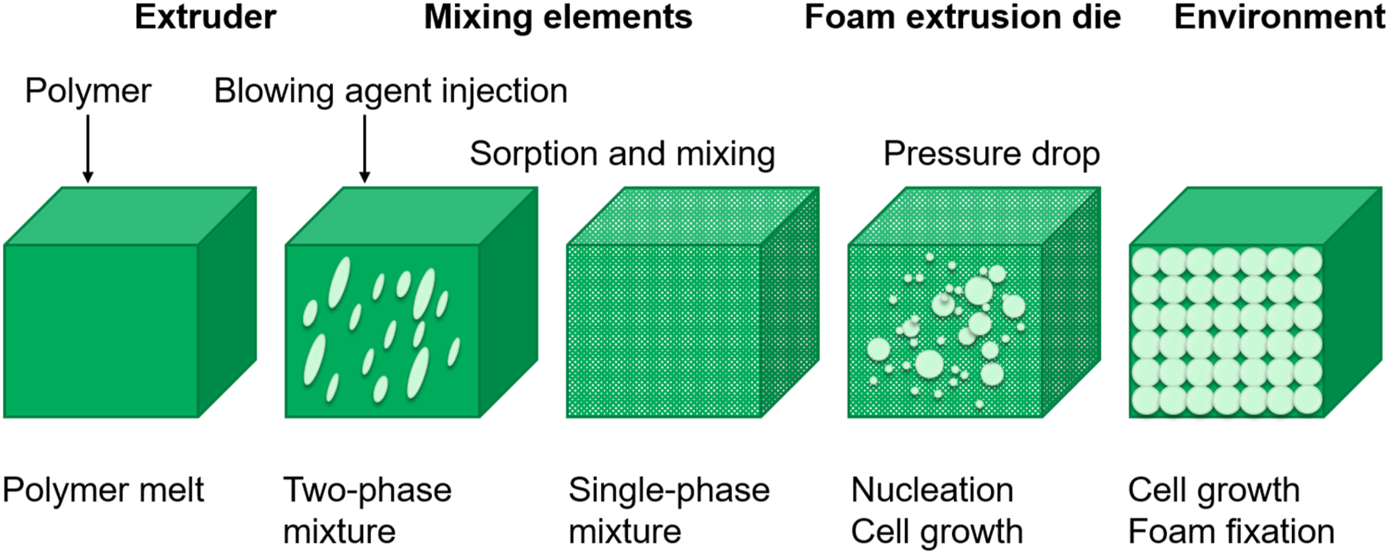

After leaving the extrusion die, foaming of the extrudate continues until the foam structure is solidified. Important parameters for successful formation of cells is the complete dissolution of the blowing agent in the melt, the creation of a high number of nuclei due to the pressure drop as well as the kinematics of cell growth and diffusion of blowing agent into the cells.^12,28

Modelling flow and foaming in the extrusion die

When modelling foam extrusion, different phenomena have to be taken into account. Besides material properties, nucleation and cell growth, the flow field in the die gap should be considered.²¹ Additionally, further effects like the shear rate can be taken into account.^7,57

Based on the works of Baldwin et al. and Stephen et al. a foam extrusion model can be set up using process data like temperature, flow rate, blowing agent concentration, information on die geometry and initial material data like viscosity, surface tension, density, solubility and diffusivity coefficients.^35,39

Based on these initial parameters, the model calculation can be carried out in steps along the flow channel, respecting the change of material properties like viscosity, surface tension and solubility due to the formation of cells and the change of gas pressure in the cells. The volume flow rate, shear rate and pressure gradient calculated for each segment of the flow channel can be used to calculate the full pressure profile along the flow channel or to calculate dimensionless numbers to describe the foaming process in the extrusion die, as it was done by Hendriks for an annular gap die.^35,39,21

The modelling approach is therefore dependent of the material properties and the PBA used, as the blowing agent load influences the material behaviour. To set up foam extrusion models, experimental data, e.g. from rheometer or solubility experiments, are therefore often combined with literature data, for example, specific density data.^35,39,21

One of the specific material properties needed for setting up a material model is the diffusion coefficient, which can be used in an Arrhenius approach to consider the temperature dependence

D (T) = D_{0} e^{- \frac{Δ E_{D}}{R T}}

(1)

Experimental data are available for the diffusion coefficients of CO₂ and N₂ in PP and other polymers, mainly from measurements with a sorption cell. Sato et al. measured solubilities of CO₂ and N₂ in molten PP and high-density polyethylene (HDPE) at temperatures of 433 K, 453 K and 473 K and pressures up to 17 MPa.⁴¹ Diffusion coefficients were determined for nitrogen in PP and HDPE and for CO2 in HDPE at 453.2 K. Other literature data for diffusion coefficients of CO₂ can be found from Durril und Griskey⁴² for various polymers and from Areerat et al. for CO₂ in LDPE, HDPE, PP, EEA and PS.⁵⁸ For novel blowing agents or blowing agent mixtures, there is often no experimental data for diffusion coefficients in the literature. This may be due to the high experimental effort for extensive series of measurements with various blowing agents under different process conditions.

Fundamentals of the diffusion of small penetrant molecules in polymers and their determination by MD simulations

Diffusion process

The diffusion process of a small penetrant molecule in glassy or rubbery polymers is widely described in literature as a so-called ‘hopping’ mechanism.^59–64 This mechanism can be divided in to two types of motion. The first one is the oscillation of the penetrant molecule in a microcavity in the polymer matrix. The duration of this quasi-stationary period depends on the polymer/penetrant combination. This first motion is interrupted by a ‘jump’ of the penetrant to another cavity in the polymer matrix. This is done through a ‘tunnel’ that is opened by the thermal motion of the polymer chains. In this manner, the diffusion in glassy or rubbery polymers is a combination of these two motions, while in rubbery state one might find a higher mobility of the chains and hence a higher ‘jump’ frequency. This also applies for the glass transition temperature (T_g) of glassy polymers, since for a given temperature the chain mobility for different polymers with different T_g decreases relatively with higher T_g values. This decrease in chain mobility hence leads to a decrease in the diffusion coefficient for the polymer with a higher T_g. For CO₂ in different silicone polymers, it could be shown that the number of ‘jumps’ performed decreases in the order in which T_g increases.⁶² Another important factor is the size of the penetrant. For the examples of H₂, O₂ and CH₄ it was shown that the possibility of a ‘jump’ decreases with increasing size of the penetrant molecule and thus the diffusion coefficient becomes smaller with increasing size of the penetrant.⁶³

The described ‘hopping’ mechanism undergoes a transition to a so-called ‘liquid-like’ mechanism for elevated temperatures, which leads to faster movement of the penetrant through the polymer.^48,65,66 This is due to the fact that the chain mobility in the polymer increases with increasing temperature.

Since the diffusion coefficients obtained in this work are all simulated at elevated temperatures, it is expected for the penetrant to rather follow a ‘liquid-like’ diffusion than a ‘hopping’ mechanism, although ‘hopping’ should not be completely overcome, due to the long chain length of the polymer.

Calculation of diffusion coefficients from molecular dynamics simulations

The diffusion coefficient can be obtained from the well-known Einstein relation,⁶⁷ by determining the slope of the mean square displacement (MSD) over time. The MSD is given by the following equation

〈 r^{2} 〉 = 〈 {(r (t) - r (0))}^{2} 〉

(2)

where

〈 r^{2} 〉

is the MSD and

r

the position vector of the diffusing particle. If the simulation time is long enough, the diffusion coefficient is described by the following equation⁶⁸

D = \frac{1}{6} \lim_{t \to \infty} 〈 \frac{d}{d t} {(r (t) - r (0))}^{2} 〉

(3)

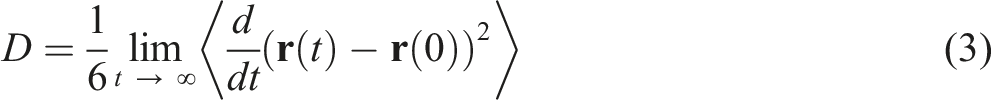
Here D is the self-diffusion coefficient, t is the time, r(t) is the position vector of the penetrant molecule at time t and the angle brackets give the ensemble average. As already mentioned, this relation is only valid for sufficiently long simulation times. In the literature, 1–2 nanoseconds (ns) is described as a sufficiently long simulation time when the diffusion coefficient is around 10⁻⁶ cm²/s.^50,66 Since the diffusion coefficients calculated in this work are all higher than 10⁻⁶ cm²/s, a simulation time of 1 ns can be considered as sufficient. Due to the ‘hopping’ mechanism described above, insufficient long monitored time period can lead to the observation of an anomalous diffusion regime, which is caused by the structure of the polymer matrix. The motion of the penetrant is restricted by the polymer matrix on the length scale of a few hopping distances and therefore cannot be truly random, resulting in anomalous diffusion.⁶³ This means the determined diffusion coefficients have to be treated with great caution and a truly Einstein behaviour has to be ensured, which can be done by a double logarithmic plot of the MSD vs. t. With this plot it can be checked that the MSD follows a power law regime, $〈 r^{2} 〉 \propto t^{n}$ with n $= 1$ , which is close to unity.⁶³ This verification is necessary because it is known that anomalous diffusion occurs if the simulation time is not long enough, which leads to $n < 1$ .⁶⁹ Further, it was found that the determination of the exact nature of the diffusion regime is of even more importance for time areas where the MSD have not reached the value of the simulation box size L squared. So, it should be checked that for the case of MSD smaller than the edge length L of the simulation box squared, MSD ∼ t¹ holds true.⁷⁰

Methodology

All simulations in this work were performed with the BIOVIA Materials Studio software. A polymer chain of isotactic polypropylene was built, consisting of 60 monomer units. Ten of these chains with different conformations were placed in a box using the Amorphous Cell tool of Materials Studio software package. Due to computational limitations, only the amorphous configuration of isotactic polypropylene was considered. Since isotactic polypropylene is in a rubbery state at the elevated temperatures used for our simulations, these limitations do not have a major impact on the diffusion results. The described cell building led to a total of 5420 atoms in the box. About 5 weight percentage of the penetrant molecules (48 N₂, 30 CO₂ and 29 EtOH molecules) were placed in those boxes, resulting in a cubic box with a cell length of 36.5 Å (Å) for each penetrant/polymer combination. The assumption of a totally amorphous system was made due to computational limitations, but since all calculations of diffusions coefficients are done at temperatures well above the melting temperature of isotactic polypropylene the polymer melt is completely amorphous. To achieve a higher accuracy, 10 different starting configurations were created for each polymer/penetrant combination and all three temperatures, from which the results are averaged. For all simulations periodic boundary conditions were applied. The long-range nonbond interactions were treated by charge groups and a cutoff value of 12.5 Å was used. The length of the cutoff radius was chosen in a tradeoff between higher accuracy and higher computational effort. Furthermore, all simulations were carried out by using the COMPASS II force field.^71,72 The COMPASS force field is a general all-atom force field specifically suited for atomistic simulations on organic molecules, inorganic small molecules and polymers, developed through ab initio and empirical parameterisation methods.⁷¹ Since the starting structures are not in a state of equilibrium, an equilibration procedure was applied. This procedure was initiated with a geometry optimisation using the Smart algorithm, followed by a very short NpT simulation (constant number of particles N, pressure p and temperature T) for which a time step of 0.1 femtoseconds (fs) was used with a maximum total simulation time of 10 picoseconds (ps). Those short NpT simulations were performed with a pressure of 1 bar and a temperature of 298 K. The reason for these short NpT simulations was to account for close contacts between atoms that might be induced by the cell building process. Those close contacts can lead to a collapse of the simulation, when a wider step size is used. To further equilibrate the system an annealing procedure is appended, which is achieved by repeated heating and cooling of the system to faster reach the state of equilibrium. Here, the simulation cell his frequently heated and cooled in a temperature range between 250 K and 500 K, while applying an NpT ensemble. Five of such heating and cooling cycles were performed leading to a total simulation time of at least 50 ps. The last step of the equilibration procedure was a long NpT simulation of 500 ps and a time step of 1 fs, with a pressure of 1 bar and the respective temperature (453 K, 473 K and 493 K). In all NpT simulations pressure and temperature were controlled by the Berendsen method.⁷³

For the production runs, a NVE (constant number of particles N, volume V and energy E) ensemble was used, with a time step of 1 fs and a total simulation time of 1 ns for the penetrants CO₂ and N₂ and 4 ns for the system with ethanol (to account for the bigger size of the ethanol molecule). After the production runs with the NVE ensemble, the temperature deviation was checked and it was ensured that there was no temperature change during the simulation, which is to assure for the stability of the system. The first 500 ps, respectively 2000 ps for the systems with ethanol, of those simulations were used to calculate the mean square displacement of the penetrant molecules.

Results and discussion

Discussion of the diffusion results

In this chapter, the calculated diffusion coefficients for CO₂ and N₂ are compared with experimental results from literature data, while no such data could be found for ethanol. We also show the influence of temperature and penetrant size on the diffusion and find them in good agreement with other studies in this field. Table 1 lists the calculated diffusion coefficients for three different temperatures (453 K, 473 K and 493 K) and compares them with different experimental results. The diffusion coefficients were calculated from the slope of the MSD using equation (3). The simulated results are given for the three different temperatures, while the experimental results are only given for a single temperature. Column 5 shows the experimental literature values according to Sato et al.⁴¹ and column 6 the corresponding values according to Durill and Griskey.⁴² All diffusion coefficients listed, are given in units of cm²/s ∙ 10⁻⁵

Table 1.

Results of the diffusion coefficients calculated in this work and their corresponding standard deviation, as also experimental results from literature data for comparison. All diffusion coefficients listed, are given in the units of cm²/s ∙ 10⁻⁵. Where column five shows experimental results from Sato et al.⁴¹ and column six shows experimental results from Durill and Griskey⁴². In both cases, the experimental results were obtained through experiments on polypropylene.

Molecule	D_sim (T = 453 K)/10⁻⁵ cm²/s	D_sim (T = 473 K)/10⁻⁵ cm²/s	D_sim (T = 493 K)/10⁻⁵ cm²/s	D_exp (T = 453.2 K)/10⁻⁵ cm²/s⁴¹	D_exp (T = 461 K)/10⁻⁵ cm²/s⁴²
N₂	7.96 ± 0.90	9.36 ± 1.05	11.9 ± 1.27	7.3	3.51
CO₂	5.56 ± 0.88	6.43 ± 0.93	7.22 ± 1.25	—	4.25
EtOH	2.32 ± 0.27	3.02 ± 0.36	4.01 ± 0.56	—	—

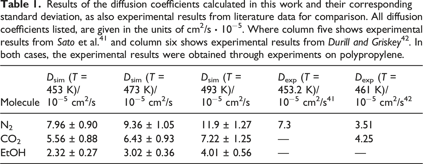
As Table 1 shows, for all three penetrant molecules the diffusion coefficients increase with increasing temperature. The comparison of the diffusion coefficients for the selected temperatures shows that the simulated results are all within the same order of magnitude as the experimental results. The diffusion coefficient for N₂ at 453.2 K estimated by Sato et al.⁴¹ shown in column five of Table 1 is quite close to the one calculated by MD simulations in this work, although the simulated diffusion coefficient at a temperature of 453 K shows a little overestimation. This overestimation becomes even higher if compared to the results of Durill and Griskey⁴² shown in column six of Table 1, but still the simulated values are in the same order of magnitude. This also applies for the diffusion coefficient of CO₂, compared to the experimental results. Also, it can be seen from the MD simulation results that the CO₂ diffusion coefficient is smaller than the diffusion coefficient of the N₂ molecules, while the diffusion coefficient of ethanol is even smaller. This results from the different size of the penetrant molecules. Since the N₂ molecule is smaller than the CO₂ molecule and the CO₂ molecule is smaller than the ethanol molecule, a different penetrant mobility is expected resulting in faster diffusion of N₂ compared to CO₂ and ethanol.⁷⁴ This can be explained by the fact that a smaller size offers the possibility to ‘jump’ through smaller tunnels and thus provides more opportunities to ‘jump’.⁶³ Same statements hold true for the diffusion coefficients of ethanol. Those coefficients are smaller for all three temperatures which was to be expected, due to the bigger size of the ethanol molecule compared to N₂ and CO₂. The tendency of decreasing diffusion coefficients with increasing molecule size is in good agreement with other MD simulation results but stays in contrast to the experimental results by Durill and Griskey.⁴² As column six in Table 1 shows, their results indicate an opposite relationship between molecular size and diffusion coefficient for N₂ and CO₂ diffusion in polypropylene, although the diffusion coefficient of CO₂ was smaller than that of N₂ in the same work for polyethylene.⁴² One reason for this deviation could be possible effects caused by the influence of gas solubility in the experiments, while in the MD simulations pure diffusion and no solubility of the penetrant is considered. Furthermore, experimental results by Kundra et al. for CO₂ in polypropylene⁷⁵ and for N₂ in polypropylene⁷⁶ again indicates the same relation between molecule size and diffusion coefficient as the MD simulations does, which could indicate a stronger dependence of the diffusion coefficient to the experimental method. But the exact reason for this deviation cannot be completely explained and would be a question to future research. Moreover, the results by Kundra et al.^75,76 agree well with those calculated by MD simulations in this work, although their values were all measured at elevated pressures. Kundra et al. give a diffusion coefficient of 2.36 ∙10⁻⁵ cm²/s⁷⁶ for CO₂ in polypropylene at a temperature of 453 K and a pressure of 2.9 bar. For N₂ in polypropylene at a temperature of 453 K and a pressure of 19,9 bar they measured a diffusion coefficient of 5.09 ∙10⁻⁵ cm²/s⁷⁵. Like the experimental values in Table 1, the diffusion coefficients of Kundra et al. are lower than the diffusion coefficients calculated from the MD simulations. In this comparison of the simulated and experimental results, one has to keep in mind the small size of the simulated system of 60 monomers and the relative short time scales of a few nanoseconds which are applied in the simulations. So the observed deviations between simulated and experimental results could be due to a finite size effect,⁶³ although there are results that indicate that the influence of the limited chain length is just a small limitation.⁵³ Müller–Plathe et al.⁵³ found only small deviations in the diffusion coefficients with increasing size of the simulation system and concluded that finite size effects play no role for the system size in question for MD simulations. The deviations in the diffusion coefficient they found are in a comparable range as those deviations found in our work between the calculated and experimental values. Other factors that might explain the differences are a not completely equilibrated system, due to the short time scales in question, or inaccuracies in the interaction potential.⁵⁰ Overall, the simulated diffusion coefficients for the single penetrant molecules all lie in the same order of magnitude compared to the experimental ones, although some deviations were found in the tendencies between penetrant size and diffusion coefficient the simulated results compare quite well with the experimental ones. Furthermore, the comparison between the different experimental results for N₂ and CO₂ from two different sources illustrates the difficulty in estimating the diffusion coefficient by experiment. Another example of these difficulties in the experimental determination of the diffusion coefficient is the fact that Durill and Griskey⁴² found a smaller diffusion coefficient for N₂ in polypropylene than Sato et al.,⁴¹ although Durill and Griskey⁴² worked at a higher temperature. Since the simulated values for CO₂ and N₂ agree well with the experimental results and trends obtained by other MD simulations, and due to the lack of experimental results for ethanol, one could compare the simulated results for ethanol with the simulated results of N₂ and CO₂. Due to the bigger size, one would expect the diffusion coefficient of ethanol to be smaller as those for CO₂ and N₂. In this respect, the diffusion coefficients of ethanol obtained in this work can be seen as reliable.

Figure 2 shows three MSD over time diagrams as an example, representing only one out of 10 starting configurations. It shows the Mean-Square-Displacement (equation (2)) of CO₂ over time in polypropylene for three different temperatures. The first 100 ps weren’t used for the evaluation, due to a clear non-linear behaviour in this time domain. This non-linear behaviour is due to the free flight of the penetrant in the microcavity at the beginning of the simulation and is of non-diffusive nature.⁵⁴

Figure 2.

MSD vs. t for the diffusion of CO₂ in polypropylene for three different temperatures.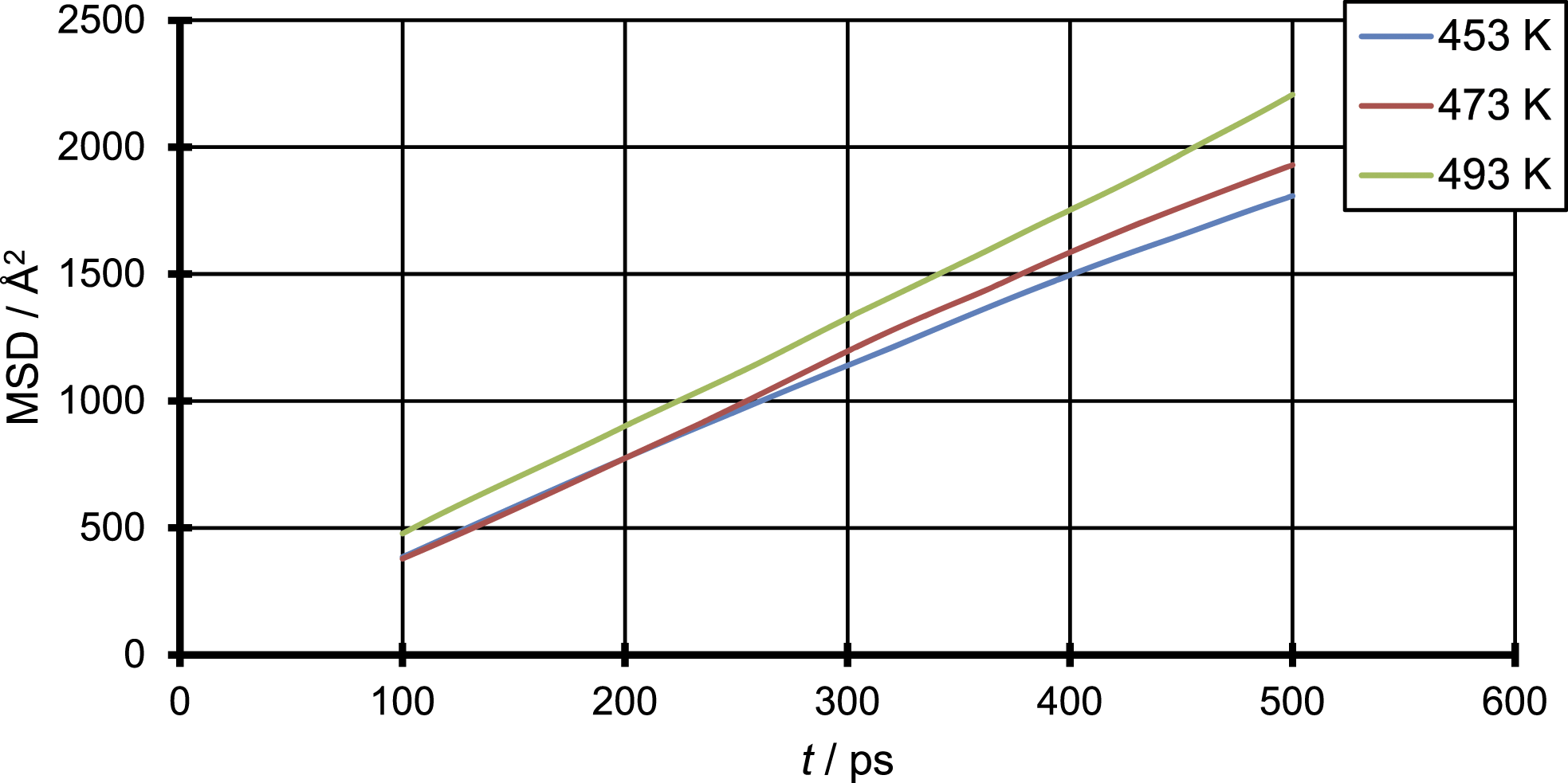

The results of the MSD show a clear linear behaviour. Furthermore, it can be seen that the MSD increases with increasing temperature, as it is expressed in the increasing diffusion coefficients. To ensure the domain of normal diffusion is reached, a double logarithmic scaled plot of MSD vs. t was created (Figure 3 gives an example for a single starting configuration) to check for linearity. As describe above, for a normal diffusion the relation, $〈 r^{2} 〉 \propto t^{1}$ has to be fulfilled. This was checked for the MSD results used to determine the diffusion coefficient and it was found that the slope is close to unity. No strong deviations found that could indicate anomalous diffusion.

Figure 3.

MSD vs. t with logarithmic scaling, to ensure the existence of a normal diffusion.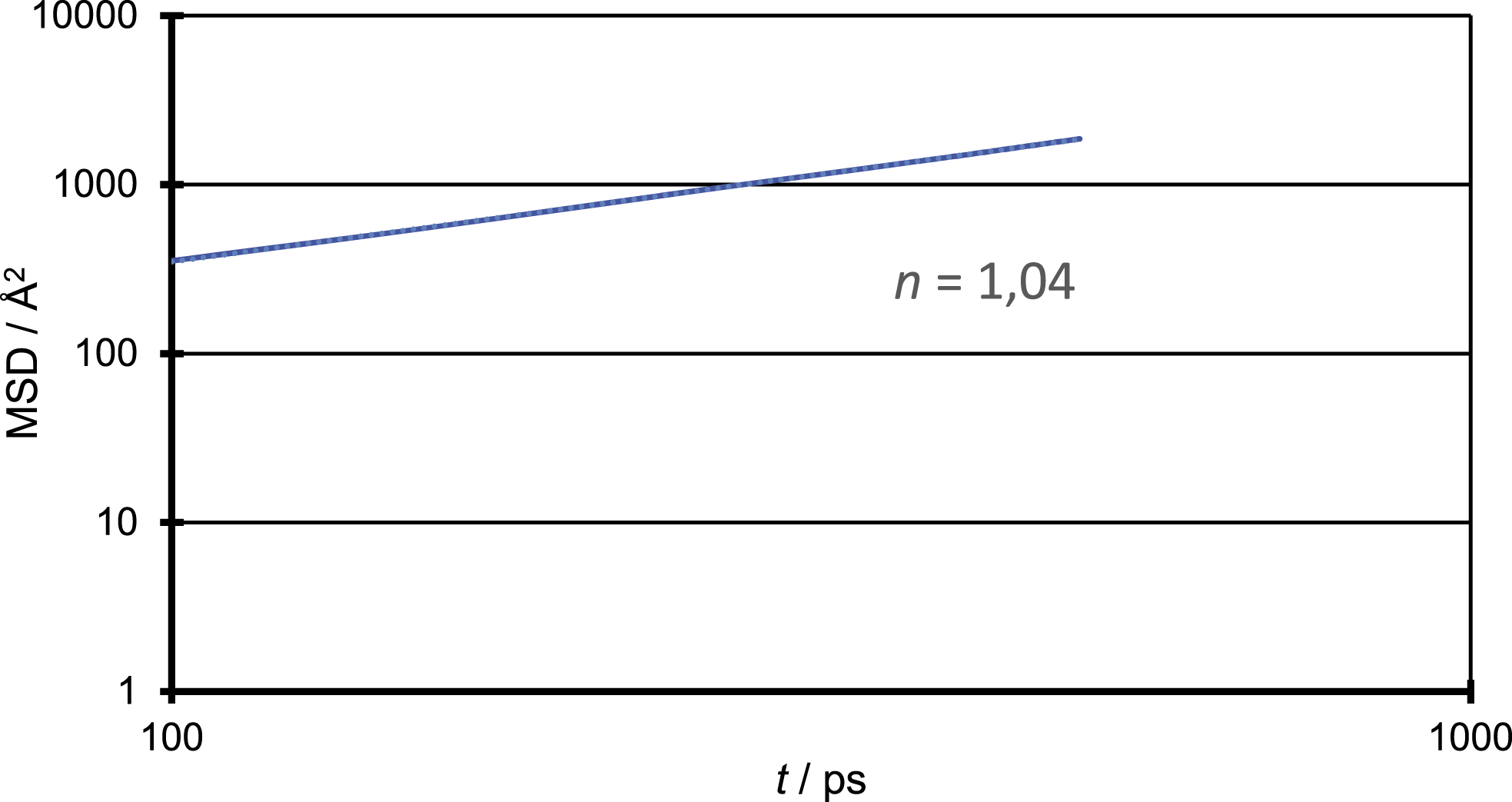

To illustrate the underlying mechanism of the diffusion in the polymer penetrant systems and compare them with findings in literature, in Figures 4 – 6, the total displacement over time is shown for all three penetrant molecules and all three temperatures. The results were generated for a single penetrant molecule, which can be viewed as representative.

Figure 4.

Total displacement of a N₂ molecule for the three different temperatures.

Figure 5.

Total displacement of a CO₂ molecule for the three different temperatures.

Figure 6.

Total displacement of an EtOH molecule for the three different temperatures.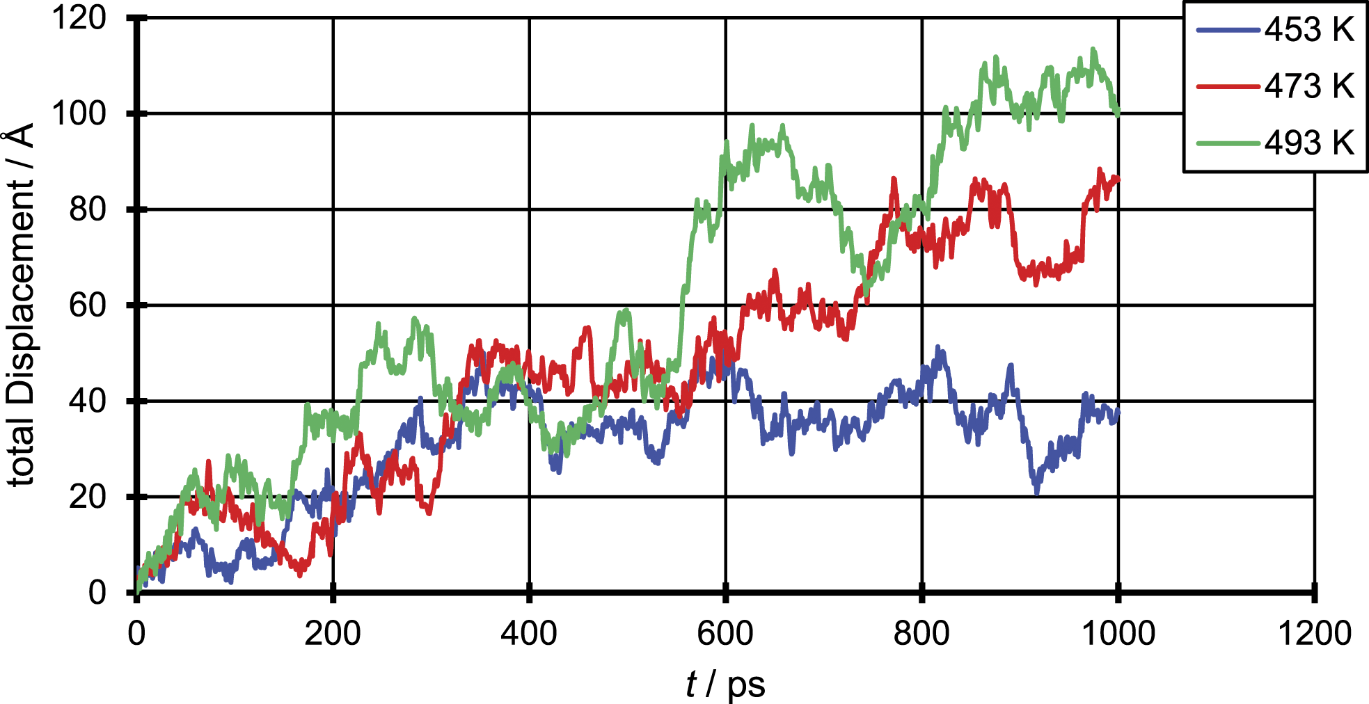

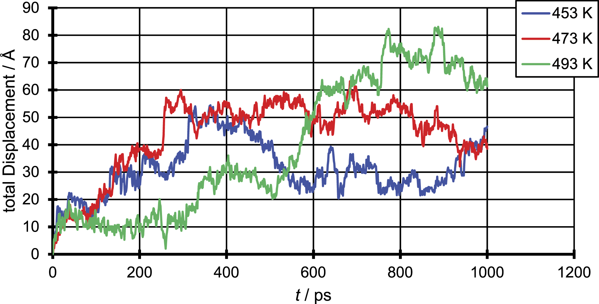
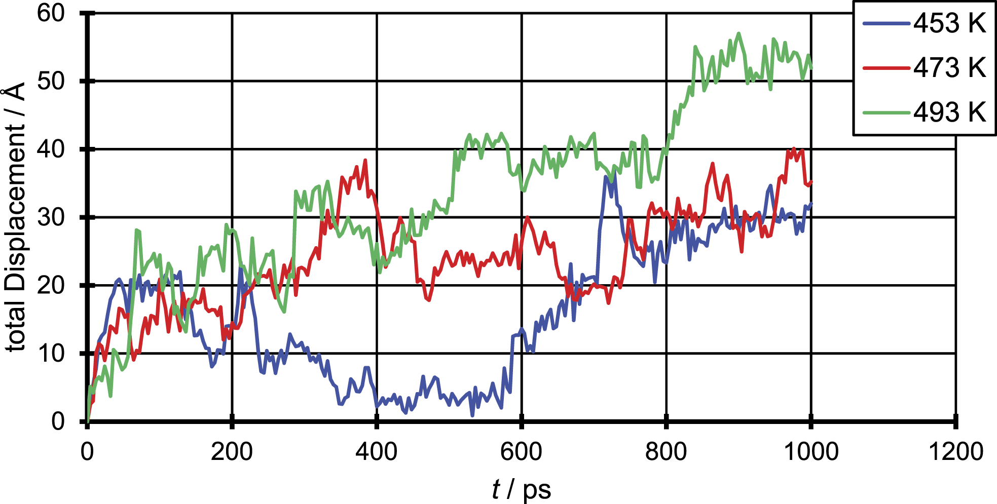
The figure of the total displacement over time shows the aforementioned dependency of the diffusion coefficient from the temperature. It can be seen that the total displacement for the chosen penetrant particle increases with higher temperatures and decreases with increasing penetrant size which in average over all penetrant molecules leads to an increase of the diffusion coefficient with increasing temperature and decreasing particle size. More important is that the total displacement over time shows that the penetrant diffusion follows a ‘hopping’ mechanism. On the one hand one can see areas of high oscillation in a range of just a few Å which correspond to the movement of the penetrant in a cavity. On the other hand, this oscillations are interrupted by bigger movements of about 10 Å which correspond the to a single jump event taken place.⁶⁹ This means even at such elevated temperatures the ‘hopping’ mechanism does not completely merge into a ‘liquid-like’ mechanism, but the number of ‘hopping’ events taken place increases and so smoothens the curve compared to simulations at room temperature. This can be due to the fact that polymers even in liquid state are quite immobile, due to the slow motion of the single chains. Instead, like in a low molecular weight fluid were the fluid velocity is of the same magnitude as the velocity of the penetrant, in a polymer system the penetrant diffusion still depends on the slower chain mobility of the polymer.⁶⁶ The above describe mechanism for the penetrant diffusion, found in this work compares well to the findings by van der Vegt⁶⁶ who invested the temperature dependence of penetrant diffusion in polyethylene. To further illustrate the temperature dependence, Figure 7 shows a 2-dimensional plot of the displacement in x and y direction, for a single N₂, CO₂ and ethanol molecule at 453 K each. As for the total displacement the single particle was chosen representative to illustrate the behaviour which is expressed in average by an increase of the diffusion coefficients.

Figure 7.

2-Dimensional representation of the total displacement.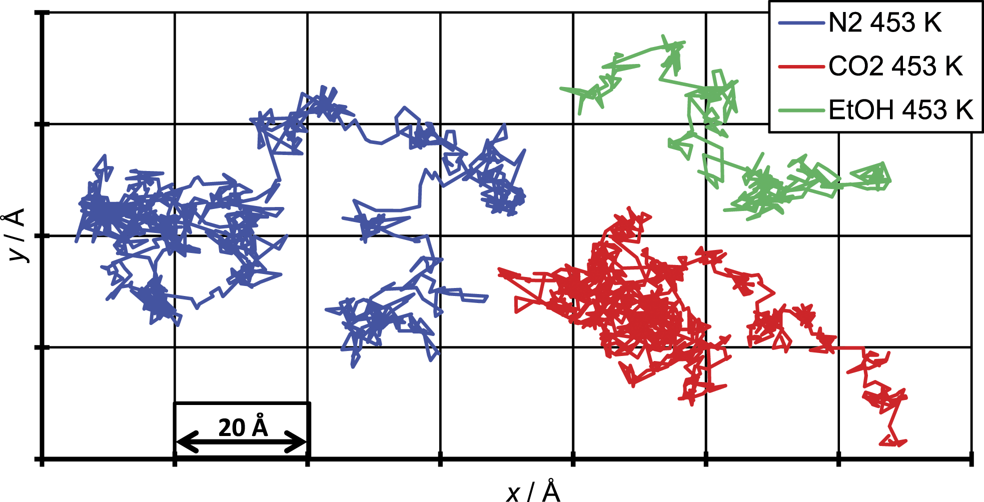

Figure 7 depicts the single jumps which has taken place while the penetrant molecule moves through the polymer matrix. For all three penetrant molecules shown here, one can also see the higher number of jumps for the N₂ molecule compared to the CO₂ and ethanol molecule, which in average is represented by the higher diffusion coefficient of the N₂ molecule.

The temperature dependence of the diffusion coefficient can be described by an Arrhenius plot following equation (1), which is shown in Figure 8.

Figure 8.

Arrhenius plot of the three penetrant molecules N₂, CO₂ and EtOH.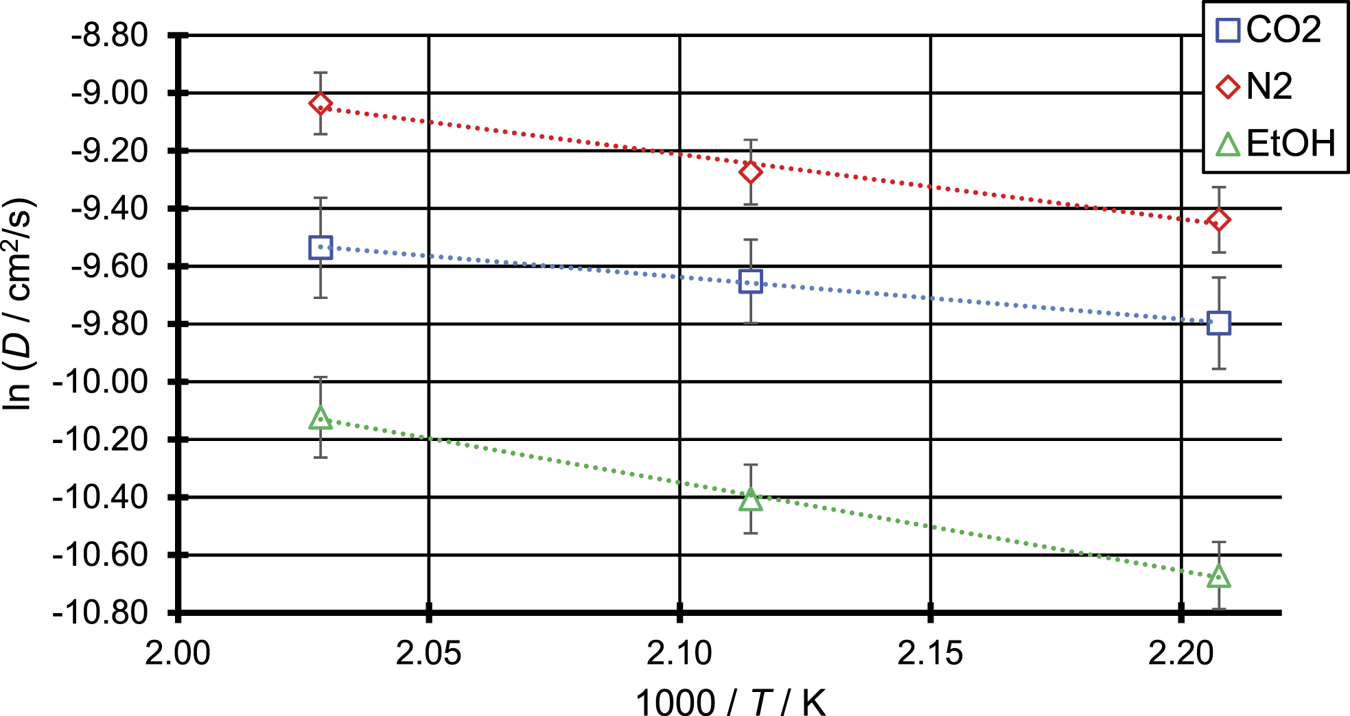

As can be seen in Figure 8 for all three penetrant molecules the diffusion coefficient shows a linear dependence with 1/T, following the Arrhenius relation. From the slope the activation energy for the diffusion of the penetrant molecule can be calculated. Those equals 18.6 kJ/mol for N₂ and 12.1 kJ/mol for CO₂. Experimental values of the activation energy by Kurek et al. are 28.8 kJ/mol and 28.2 kJ/mol for N₂ and CO₂, respectively.⁷⁷ First, it is important to mention that these experimental results were measured for a lower temperature range from about 273 K to 330 K. It was shown for polyethylene that the diffusion coefficient of penetrant diffusion does not follow an Arrhenius behaviour over the complete temperature range, but instead shows a transition in the slope between high and low temperature areas.⁶⁵ These findings could explain the discrepancy between the measured results of Kurek et al.⁷⁷ and the simulated results in this work, assuming that there is also a change in the slope of the Arrhenius plot for polypropylene, depending on the temperature range. Furthermore, since at the given experimental temperatures polypropylene is in a solid state, this might explain why the activation energies are higher than those calculated via MD simulations at temperatures above the melting point. Polypropylene underneath the melting point is a semi-crystalline polymer, which leads to a slower Diffusion, due to the assumption of the complete absence of diffusion in crystalline areas. These areas of crystallinity, which arise from the lower temperature range in which the activation energies were measured, might explain the higher activation energy for the diffusion in solid polypropylene. By further comparison of the activation energies by Kurek et al.⁷⁷ and the activation energies from MD simulations, one can find that the difference between the activation energies of N₂ and CO₂ are relatively high between these two different methods. So, the activation energy from MD simulation for N₂ is 6.5 kJ/mol higher than the activation energy of CO₂, while the difference of the activation energies from Kurek et al.⁷⁷ amounts only to 0.6 kJ/mol. An explanation for these differences might again be the different temperature range. Another reason could be that the deviations arise from the MD simulations itself, which would demand the need for further calculations in a lower temperature range for direct comparison. The simulated results of this work could also be compared to results for CO₂ diffusion in polyethylene, since polyethylene and polypropylene show a high chemical likeliness. For the CO₂ diffusion in a high temperature range, which is comparable to the temperature range viewed in this work, for CO₂ diffusion in polyethylene, an activation energy of about 15 kJ/mol was found.⁶⁶ This literature value is close to the one found here for the CO₂ diffusion in polypropylene. These comparisons with the literature show a high reliability of the simulated activation energies found in this work.

For ethanol as the penetrant molecule, an activation energy of 25.4 kJ/mol is found. This is significantly higher than the activation energies of N₂ and CO₂ which was to be expected, due to the bigger size of the ethanol molecule compared to the other two penetrant molecules. In contrast to this result the activation energy of N₂ determined from MD simulations is higher than the activation energy obtained for CO₂, although N₂ is the smaller molecule. This result is consistent with the activation energies Kurek et al.⁷⁷ received, although their results show a smaller difference between the activation energies of N₂ and CO₂. As mentioned above, this is a question for future research. Hence, as already done for the diffusion coefficient the quality of the activation energy of ethanol can be judged by the comparison with the other two penetrant molecules. Due to the larger size of the ethanol molecule, the observed deviations to a higher activation energy would be expected, so that the simulated activation energy of ethanol appears reliable.

Conclusion

For modelling foam extrusion processes, knowledge of the diffusion behaviour of the blowing agent in the molten polymer is crucial. As an alternative to experimental methods, molecular dynamics (MD) simulations were used to calculate the diffusion coefficients of the penetrant molecules N₂, CO₂ and ethanol in polypropylene at elevated temperatures. The calculated diffusion coefficients were found to be in the same order of magnitude as those described in literature obtained from solubility experiments. Only for the relation between penetrant size and diffusion coefficient the experimental results by Durill and Griskey⁴² show an opposite trend as the simulated results does, for which the reason is a question to further research. Furthermore, the diffusion mechanism was investigated and found to correspond well to the mechanism of action described in literature as ‘hopping’ mechanism with a slight transition through a ‘liquid-like’ mechanism. Also, the temperature dependence of the diffusion process was evaluated and found to be linear, following the known Arrhenius-like behaviour. From those evaluations the activation energies were extracted and compared to experimental and simulated values. Here, the agreement between the literature data and the results from this work showed a deviation, since in the experiments higher activation energies were found. This deviation could be explained by the different temperature ranges in which the diffusion process was monitored in experiment and simulation. This conclusion is fortified by results of the activation energy of CO₂ diffusion in polyethylene. Since polyethylene has high chemical likeliness compared to polypropylene, it can be expected that the activation energies are similar, which is found by the comparison between literature data and our simulations.

Overall, the MD simulations allowed to calculate diffusion coefficients at elevated temperatures, which agreed well with experimentally determined diffusion coefficients, except for the deviations mentioned before. Thus, MD simulations can be a valuable tool in calculating diffusion coefficients for blowing agents and blowing agent mixtures allowing predictions of the solubility for foam extrusion processes. Especially when novel blowing agents or blowing agent mixtures are used, this is helpful because experimentally determined diffusion coefficients cannot be found in literature yet. The next step would be to expand the MD simulations to other blowing agents like acetone or isopropanol and to different combinations of these blowing agents as blowing agent mixtures. For modelling foam extrusion, MD simulations offer promising possibilities to improve the model quality and enhance the precision of calculated material data from these models without the need to run extensive series of experiments. The findings allow to calculate diffusion coefficients independently from experimental for various combinations of blowing agents and polymers at elevated temperatures and pressures, allowing sophisticated models to be set up faster and easier in the future.

Footnotes

Acknowledgments

Computational results were obtained by using Dassault Systèmes BIOVIA software programs. BIOVIA Materials Studio was used to perform the calculations and to generate the graphical results.

Declaration of conflicting interests

The author(s) declared no potential conflicts of interest with respect to the research, authorship, and/or publication of this article.

Funding

The author(s) disclosed receipt of the following financial support for the research, authorship, and/or publication of this article: Funded by the Deutsche Forschungsgemeinschaft (DFG, German Research Foundation) under Germany’s Excellence Strategy - EXC-2023 Internet of Production - 390621612.

ORCID iDs

Felix Melzer

Robert Breuer

References

Klempner

Frisch

(eds). Handbook of polymeric foams and foam technology. Munich: Hanser; 1991.

Lee

Park

. Foam Extrusion: Principles and Practice. 2nd ed. Boca Raton: Taylor & Francis, 2014.

Tomasko

Liu

, et al. A review of CO2 applications in the processing of polymers. Ind Eng Chem Res 2003; 42: 6431–6456.

Park

Baldwin

Suh

. Effect of the pressure drop rate on cell nucleation in continuous processing of microcellular polymers. Polym Eng Sci 1995; 35: 432–440.

Wong

Park

. The effects of extensional stresses on the foamability of polystyrene-talc composites blown with carbon dioxide. Chem Eng Sci 2012; 75: 49–62.

Chen

Sheth

Wang

. Effects of shear stress and pressure drop rate on microcellular foaming process. J Cell Plastics 2001; 37: 353–363.

Lee

S-T

. Shear effects on thermoplastic foam nucleation. Polym Eng Sci 1993; 33: 418–422.

Naguib

Park

Reichelt

. Fundamental foaming mechanisms governing the volume expansion of extruded polypropylene foams. J Appl Polym Sci 2004; 91: 2661–2668.

Leung

Wong

Wang

, et al. Mechanism of extensional stress-induced cell formation in polymeric foaming processes with the presence of nucleating agents. J Supercrit Fluids 2012; 63: 187–198.

10.

Park

. Effects of the die geometry on the expansion of polystyrene foams blown with carbon dioxide. J Appl Polym Sci 2008; 109: 3329–3336.

11.

Park

, et al. Effects of die geometry on cell nucleation of PS foams blown with CO2. Polym Eng Sci 2003; 43: 1378–1390.

12.

Kropp

. Extrusion thermoplastischer Schäume mit alternativen Treibmitteln. PhD Thesis. Germany: RWTH Aachen, 1999.

13.

Nam

Yoo

Lee

. Effect of long-chain branches of polypropylene on rheological properties and foam-extrusion performances. J Appl Polym Sci 2005; 96: 1793–1800.

14.

Laguna-Gutierrez

van Hooghten

Moldenaers

, et al. Understanding the foamability and mechanical properties of foamed polypropylene blends by using extensional rheology. J Appl Polym Sci 2015; 132: 1–14.

15.

Geissler

Feuchter

Laske

, et al. Strategies to improve the mechanical properties of high-density polylactic acid foams. J Cell Plastics 2014; 52: 15–35.

16.

Zhang

Parent

Kontopoulou

, et al. Foaming of reactively modified polypropylene: effects of rheology and coagent type. J Cell Plastics 2014; 51: 505–522.

17.

Krupinski

McLoughlin

. Low Density HMS Polypropylene Foam: Controlling Foam Density and Cell Morphology ANTEC 2017 - Anaheim, 2017. CA, USA May.

18.

Fan

Wan

Gao

, et al. Extrusion foaming of poly(ethylene terephthalate) with carbon dioxide based on rheology analysis. J Cell Plastics 2015; 52: 277–298.

19.

Stafford

Russell

McCarthy

. Expansion of polystyrene using supercritical carbon dioxide: effects of molecular weight, polydispersity, and low molecular weight components. Macromolecules 1999; 32: 7610–7616.

20.

Eaves

. Shawbury, Shrewsbury. In: Handbook of polymer foams. Shropshire, U.K: Rapra Technology; 2004.

21.

Hendriks

. Experimentelle Untersuchungen zur Schaumextrusion mit Treibmittelgemischen und Analyse der Wirkzusammenhänge mit dimensionslosen Kennzahlen (Experimental study on the foam extrusion with blowing agent mixtures and analysis of the correlations with dimensionless numbers)PhD Thesis. Germany: RWTH Aachen, 2018.

22.

Welsh

. Polystyrene foam made with only carbon dioxide as a blowing agent and a process for making the same. Patent 1993; 5. USA: 250–577.

23.

Binder

Kocsis

. Low density styrene polymer foams and process for preparing same. Patent 1993; 5. USA: 271.

24.

Institut Bauen und Umwelt e.V. Extruded Polystyrene (XPS) Foam Insulationwith alternative flame retardant. Environmental Product Declaration, 2019, p.1–9.

25.

Gendron

Vachon

Champagne

, et al. (eds). Foam extrusion of PS blown with a mixture of HFC-134a and isopropanol. In: Rapra Blowing Agents & Foaming Processes. Munich, Germany; 2003, pp. 19–20.

26.

Daigneault

Gendron

. Blends of CO2 and 2-ethyl hexanol as replacement foaming agents for extruded polystyrene. J Cell Plastics 2001; 37: 262–272.

27.

Gendron

Champagne

Delaviz

, et al. Foaming polystyrene with a mixture of CO2 and ethanol. J Cell Plastics 2006; 42: 127–138.

28.

Leung

. Mechanisms of Cell Nucleation, Growth, and Coarsening in Plastic Foaming: Theory, Simulation, and Experiment. Canada: PhD Thesis, University of Toronto, 2009.

29.

Wong

Mark

Hasan

, et al. The synergy of supercritical CO2 and supercritical N2 in foaming of polystyrene for cell nucleation. J Supercrit Fluids 2014; 90: 35–43.

30.

Zhang

Zhu

Lee

. Extrusion foaming of polystyrene/carbon particles using carbon dioxide and water as co-blowing agents. Polymer 2011; 52: 1847–1855.

31.

Pallay

Kelemen

Berghmans

, et al. Expansion of polystyrene using water as the blowing agent. Macromolecular Mater Eng 2000; 275: 18–25.

32.

Lee

Naguib

Park

, et al. Increase of open-cell content by plasticizing soft regions with secondary blowing agent. Polym Eng Sci 2005; 45: 1445–1451.

33.

Kim

Kweon

Romero-Diez

, et al. Effects of pressure drop rate and CO 2 content on the foaming behavior of newly developed high-melt-strength polypropylene in continuous extrusion. J Cel Plast 2021; 57: 413–432.

34.

Yao

Qiu

, et al. Influence of molecular structure on the rheological properties and foamability of long chain branched polypropylene by “one-pot” reactive extrusion. J Cel Plast 2021; 57: 433–449.

35.

Baldwin

Park

Suh

. Microcellular sheet extrusion system process design models for shaping and cell growth control. Polym Eng Sci 1998; 38: 674–688.

36.

Baldwin

Park

Suh

. An extrusion system for the processing of microcellular polymer sheets: shaping and cell growth control. Polym Eng Sci 1996; 36: 1425–1435.

37.

Shafi

Lee

Flumerfelt

. Prediction of cellular structure in free expansion polymer foam processing. Polym Eng Sci 1996; 36: 1950–1959.

38.

Shafi

Joshi

Flumerfelt

. Bubble size distributions in freely expanded polymer foams. Chem Eng Sci 1997; 52: 635–644.

39.

Stephen

Bhattacharya

Khan

. Mathematical modeling and numerical simulation for nucleated solution flow through slit die in foam extrusion. Polym Eng Sci 2006; 46: 751–762.

40.

Shafi

Flumerfelt

. Initial bubble growth in polymer foam processes. Chem Eng Sci 1997; 52: 627–633.

41.

Sato

Fujiwara

Takikawa

, et al. Solubilities and diffusion coefficients of carbon dioxide and nitrogen in polypropylene, high-density polyethylene, and polystyrene under high pressures and temperatures. Fluid Phase Equilibria 1999; 162: 261–276.

42.

Durrill

Griskey

. Diffusion and solution of gases in thermally softened or molten polymers: part I. development of technique and determination of data. AIChE J 1966; 12: 1147–1151.

43.

Gubbins

Moore

. Molecular modeling of matter: impact and prospects in engineering. Ind Eng Chem Res 2010; 49: 3026–3046.

44.

Maginn

Elliott

. Historical perspective and current outlook for molecular dynamics as a chemical engineering tool. Ind Eng Chem Res 2010; 49: 3059–3078.

45.

Hofmann

Tocci

. Molecular modeling, a tool for the knowledge-based design of polymer-based membrane materials. In: Drioli

Giorno

(eds). Membrane Operations. John Wiley & Sons; 2009, pp. 3–18.

46.

Kildsig

Park

. Computer simulation of molecular diffusion in amorphous polymers. J Controlled Release 1997; 48: 57–66.

47.

Kupgan

Abbott

Hart

, et al. Modeling amorphous microporous polymers for CO2 capture and separations. Chem Rev 2018; 118: 5488–5538.

48.

Han

Boyd

. Small-molecule penetrant diffusion in hydrocarbon polymers as studied by molecular dynamics simulation. Macromolecules 1994; 27: 5365–5370.

49.

Cuthbert

Wagner

Paulaitis

, et al. Molecular dynamics simulation of penetrant diffusion in amorphous polypropylene: diffusion mechanisms and simulation size effects. Macromolecules 1999; 32: 5017–5028.

50.

Meunier

. Diffusion coefficients of small gas molecules in amorphous cis-1,4-polybutadiene estimated by molecular dynamics simulations. J Chem Phys 2005; 123: 134906.

51.

Dutta

Bhatia

. Transport diffusion of light gases in polyethylene using atomistic simulations. Langmuir 2017; 33: 936–946.

52.

Volgin

Larin

Abad

, et al. Molecular dynamics simulations of fullerene diffusion in polymer melts. Macromolecules 2017; 50: 2207–2218.

53.

Mueller-Plathe

Rogers

van Gunsteren

. Diffusion coefficients of penetrant gases in polyisobutylene can be calculated correctly by molecular-dynamics simulations. Macromolecules 1992; 25: 6722–6724.

54.

Müller-Plathe

Rogers

van Gunsteren

. Computational evidence for anomalous diffusion of small molecules in amorphous polymers. Chem Phys Lett 1992; 199: 237–243.

55.

Gibbs

. The scientific papers of JW Gibbs. New York: DoverLongmans, Green and Company, 1961.

56.

Leung

Park

. Numerical simulation of polymeric foaming processes using modified nucleation theory. Plastics, Rubber and Composites 2006; 35: 93–100.

57.

Chen

Wang

Straff

, et al. Shear stress nucleation in microcellular foaming process. Polym Eng Sci 2002; 42: 1151–1158.

58.

Areerat

Funami

Hayata

, et al. Measurement and prediction of diffusion coefficients of supercritical CO2 in molten polymers. Polym Eng Sci 2004; 44: 1915–1924.

59.

Sonnenburg

Gao

Weiner

. Molecular dynamics simulations of gas diffusion through polymer networks. Macromolecules 1990; 23: 4653–4657.

60.

Takeuchi

. A jump motion of small molecules in glassy polymers: a molecular dynamics simulation. J Chem Phys 1990; 93: 2062–2067.

61.

Müller‐Plathe

. Diffusion of penetrants in amorphous polymers: a molecular dynamics study. J Chem Phys 1991; 94: 3192–3199.

62.

Charati

Stern

. Diffusion of Gases in Silicone Polymers: Molecular Dynamics Simulations. Macromolecules 1998; 31: 5529–5535.

63.

Gusev

Müller-Plathe

van Gunsteren

, et al. Dynamics of small molecules in bulk polymers. In: Abe

Benoit

Cantow

H-J

, et al. (eds). Atomistic Modeling of Physical Properties. Berlin, Heidelberg: Springer Berlin Heidelberg; 1994, pp. 207–247.

64.

Theodorou

. Principles of molecular simulation of gas transport in polymers. In: Yampolskii

Pinnau

Freeman

(eds). Materials Science of Membranes for Gas and Vapor Separation. John Wiley & Sons; 2006, pp. 49–94.

65.

Pant

PVK

Boyd

. Molecular-dynamics simulation of diffusion of small penetrants in polymers. Macromolecules 1993; 26: 679–686.

66.

van der Vegt

NFA

. Temperature dependence of gas transport in polymer melts: molecular dynamics simulations of CO2 in polyethylene. Macromolecules 2000; 33: 3153–3160.

67.

Einstein

. Über die von der molekularkinetischen theorie der wärme geforderte bewegung von in ruhenden flüssigkeiten suspendierten teilchen. Annalen der Physik 1905; 322: 549–560.

68.

Allen

Tildesley

. Computer Simulation of Liquids. 2nd ed. Oxford, United Kingdom: Oxford University Press, 2017.

69.

Hofmann

Fritz

Ulbrich

, et al. Detailed-atomistic molecular modeling of small molecule diffusion and solution processes in polymeric membrane materials. Macromolecular Theor Simulations 2000; 9: 293–327.

70.

Greenfield

. Representing polymer molecular structure using molecular simulations for the study of liquid sorption and diffusion. Curr Opin Chem Eng 2020; 28: 144–151.

71.

Sun

. COMPASS: an ab initio force-field optimized for condensed-phase applicationsoverview with details on alkane and benzene compounds. The J Phys Chem B 1998; 102: 7338–7364.

72.

Sun

Jin

Yang

, et al. COMPASS II: extended coverage for polymer and drug-like molecule databases. J Mol Model 2016; 22: 47.

73.

Berendsen

HJC

Postma

JPM

van Gunsteren

, et al. Molecular dynamics with coupling to an external bath. J Chem Phys 1984; 81: 3684–3690.

74.

Müller‐Plathe

. Molecular dynamics simulation of gas transport in amorphous polypropylene. J Chem Phys 1992; 96: 3200–3205.

75.

Kundra

Upreti

Lohi

, et al. Experimental determination of composition-dependent diffusivity of carbon dioxide in polypropylene. J Chem Eng Data 2011; 56: 21–26.

76.

Kundra

Upreti

Lohi

, et al. Experimental determination of concentration dependence of nitrogen diffusivity in polypropylene. J Appl Polym Sci 2011; 121: 2828–2834.

77.

Kurek

Klepac

Ščetar

, et al. Gas barrier and morphology characteristics of linear low-density polyethylene and two different polypropylene films. Polym Bull 2011; 67: 1293–1309.