
Abstract
Abstract
Probability and random processes is considered by students to be conceptually one of the most difficult subjects in the undergraduate electrical and computer engineering curriculum. There are numerous reasons for this difficulty encountered by the students. First off, humans are not innately good at probabilistic intuition. Traditionally, this subject has been introduced in a very abstract manner without emphasis on real-world applications from electrical and computer engineering discipline. In addition, extensive use of interactive simulation and visualization tools, offering an alternative way of developing probabilistic intuition, is usually missing from traditional course offerings. This paper presents a unique pedagogical approach to teaching an introductory probability course offered to electrical and computer engineering juniors. The salient features of the proposed pedagogical approach include more emphasis on real-world electrical and computer engineering problems that show the applications of abstract probabilistic concepts; extensive hands-on and interactive MATLAB® simulations of real-world electrical and computer engineering problems that are tightly integrated into the curriculum; highlighting the frequentist approach to build probabilistic intuition using simulations; concrete examples showing how naive probabilistic intuition can be erroneous and how to develop correct probabilistic intuition based on systematically modeling, simulating, and analyzing a problem; and application-based simulations driving the abstract theory rather than the other way around. This pedagogical approach was implemented in a course offered to electrical and computer engineering undergraduates at Purdue University Northwest. The paper presents a concrete example illustrating how the salient features of the proposed pedagogical approach were implemented as part of this course and student data from the courses to validate the efficacy of the proposed approach.
Introduction
Probability and random processes is an important course in the undergraduate electrical and computer engineering (ECE) curriculum. The importance of this course stems from the fact that it serves as a gateway to the areas of electrical engineering such as communications, signal processing, controls, and networking. Without a good understanding of probabilistic modeling and analysis techniques, a student faces considerable difficulty in the future courses in these areas. No wonder that probability and random processes is offered as a core course in the undergraduate ECE curriculum. Despite its importance, students often find this subject difficult to grasp and fail to develop the motivation to pursue areas of electrical engineering that are heavily dependent on it. 1 There are numerous reasons for comprehension difficulties of this subject encountered by the students.
Due to a strong emphasis on Newtonian mechanics in early engineering education, students are trained to conceptualize and solve deterministic problems. Almost all of the math and physics courses that undergraduate engineering students take in the first two years deal with modeling and analyzing the deterministic world. In addition, introductory electrical engineering courses like digital logic and circuit analysis do not deal with random noisy signals and their effects. Not only is their inadequate exposure and training to solve problems involving uncertainty, but humans, innately, do not tend to do be good at probabilistic intuition.2 –4 A classic illustration of this is the Monty Hall problem, which even Paul Erdös, one of the most prolific mathematicians, got initially wrong. 5
Historically, this subject has been taught in a very abstract manner without emphasis on concrete applications from ECE discipline and on modern simulation and visualization tools. Most of the examples covered in the textbooks are of generic nature that fail to provide a deeper insight and motivate ECE students to study this subject.6 –9 Occasionally, when applications of probability in ECE are presented in textbooks or courses, they are presented in a very non-interactive and terse manner without the aid of modern simulation and visualization tools, giving students a deeper intuitive understanding of the subject.6 –9
Since probability is taught using the axiomatic approach, emphasis is not placed on the frequentist approach, which even though mathematically not very desirable, can help to build probabilistic intuition. In addition, modern simulation and visualization tools such as MATLAB®, 10 GNU Octave, 11 R, 12 and Mathematica® 13 offer a hands-on and interactive way to develop probabilistic intuition, something that is usually missing from traditional course offerings.
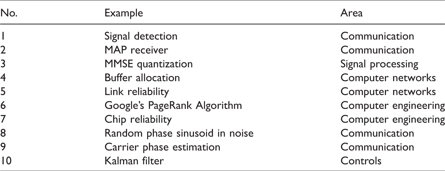
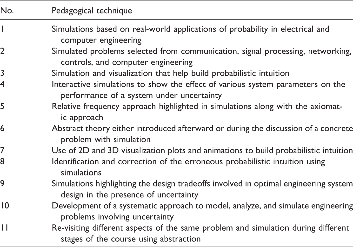
This paper presents the results from a unique pedagogical approach to teaching an introductory probability and random processes course to ECE juniors. The unique pedagogical features of this course include more emphasis on real-world ECE problems from the areas of communication, signal processing, networking, controls, and computer engineering, listed in Table 1, that show the applications of abstract probabilistic concepts; extensive hands-on and interactive MATLAB® simulations of real-world ECE problems highlighting the frequentist approach to build probabilistic intuition; concrete examples showing the fallacies and pitfalls of naive probabilistic intuition, and how to systematically develop correct intuition by doing the appropriate math and validate it through simulations; less time spent on theory and more on solving problems and applications; revisiting different aspects of the same bigger problem during different parts of the course and using abstraction to hide details that depend upon material that has not been covered yet; and highlighting the tradeoffs involved in the design of optimal engineering systems under uncertainty. A complete list of these pedagogical features is shown in Table 2.
Real-world applications of probability in electrical and computer engineering.
Pedagogical techniques used in the course.
Even though MATLAB® 10 was used as the simulation software during the course due to its wide applicability in ECE curriculum, numerous other alternative simulation software tools exist, such as GNU Octave, 11 R, 12 and Mathematica® 13 that could have equally been used to develop the simulations.
The paper is organized as follows: “Related work” section presents an overview of the related work in this area. “Illustrative example (signal detection)” section presents a concrete example of signal detection to illustrate how the unique pedagogical features of Table 2 were implemented. In “Efficacy studies” section, we present student data to validate the efficacy of the proposed pedagogical techniques. Finally, we conclude the paper in “Conclusion and future work” section highlighting some future directions.
Related work
Engineering education is rapidly evolving based on the new pedagogical techniques enabled by modern computational technology. Various researchers have investigated the efficacy of such pedagogical techniques involving simulation, gaming, visualization, and virtual labs in teaching undergraduate ECE courses. Christou et al. 14 and Dinov et al. 15 describe a design for incorporating Statistics Online Computational Resource (SOCR) tool in instruction. SOCR provides various interactive tools such as statistical calculators, simulation applets, data analysis, and visualization for enhanced instruction in various undergraduate and graduate courses in probability and statistics. Their findings indicate that the effect of SOCR on the treatment group across all classes was significant. The authors concluded that employing SOCR technology enhances overall the students’ understanding and long-term knowledge retention.
Reis and Kenett 16 provide a classification of a wide range of simulation tools used in teaching statistical methods based on the level of complexity and sophistication of the courses. Viali 17 presents the assessment results from the use of a discrete event simulation software QUeuing Event Simulation Tool in a sophomore-level engineering probability and statistics course. The simulations were used to illustrate the effects of different probability distributions on the performance of a system. De Raffaele et al. 18 investigated the efficacy of implementing tangible user interfaces to improve the learning experiences of students in a queuing theory course. By augmenting simulations with a table-top architecture, the authors demonstrate real-time interaction and visualization of queuing theory concepts. Their efficacy study found a 25% increase in grades when compared with the traditional teaching methods.
Garfield et al. 19 present results from a three-month-long teaching experiment utilizing TinkerPlots™ software for statistical modeling and analysis. Their results suggest that incorporating modeling and simulation tools can develop statistical intuition. In addition, their approach seems to help students develop a better appreciation for statistics in practice.
A comprehensive topical survey of some of the most important and recent research on teaching and learning probability is presented in Batanero et al. 20 Some of the topics covered in this survey include intuition and learning difficulties in probability and educational technology resources in probability education.
A collection of the latest research in statistics education performed by international scholars is presented in Ben-Zvi and Makar. 21 The studies in this book present unique challenges that students and teachers of statistics face while learning and teaching statistics, respectively. In addition, important theoretical and techno-pedagogical challenges are also presented. The technological tools presented in this work are used to enhance creative learning, simulate abstract ideas, and experiment with statistical models.
Two recent important bodies of work in the area of application and simulation-based teaching of probability and random processes to electrical and computer engineers are Kay 22 and Walrand. 23 The book by Kay 22 presents a unique pedagogical approach of presenting motivating examples first and generalizations later to teaching probability and random processes. Even though the book takes a “hands-on” approach to teach probability by providing a comprehensive list of real-world examples and simulations from various disciplines, it is geared toward first-year graduate-level students.
The book by Walrand provides a list of representative applications that make use of a wide range of probabilistic ideas and concepts. 23 The book, however, is written for an upper-division probability course in electrical engineering and computer science and assumes that the students have taken an introductory probability course. The material is organized around applications, and each chapter starts with a real-world electrical engineering and computer science application of probability. “Hands-on” projects using MATLAB® and Simulink® are used throughout the book.
Despite the fact that, recently, there has been an increased interest in an application-based and simulation-driven pedagogical approach to teaching probability, none of the work incorporates all of the pedagogical techniques listed in Table 2. In addition, efficacy studies measuring the effectiveness of these pedagogical techniques are lacking. This paper addresses these shortcomings in the related work.
Illustrative example (signal detection)
Table 1 lists some of the real-world applications of probability and random processes in ECE that were discussed during the course. Interactive MATLAB® simulations were developed for each of these applications from communication, signal processing, networking, controls, and computer engineering. The theory was presented either side-by-side simulations and applications or afterward. Significantly, more time was spent on concrete applications and simulations than on abstract theory. Using simulations, the fallacy of the naive and erroneous probabilistic intuition was highlighted, and a systematic approach to model, analyze, and simulate a probabilistic problem was developed. Only after going through this systematic approach, the students were encouraged to develop correct probabilistic intuition. One of the challenges of using real-world ECE applications was that they relied on probabilistic ideas introduced during different parts of the course. However, this problem was circumvented by using abstraction to hide the details that rely on ideas not yet covered during the course and revisiting the same application during different parts of the course to highlight different aspects of the application. This requires certain skill on the part of the instructor on how to efficiently hide the details without compromising the necessary information needed for the problem at hand; nevertheless, the instructor was able to implement this approach quite efficiently.
Most of the application areas listed in Table 1 are covered to some extent in introductory probability textbooks for ECE majors.6 –9 So, this is not a question of introducing advanced material to the students, but rather how to more effectively present the material that is already being presented in the current textbooks. Most of the current textbooks tangentially touch these topics without sufficient details and simulations to help build a deeper understanding of the topic. This can be quite frustrating for the students who have to rely on a half-baked idea to understand a difficult concept.
In the following, we present a concrete example of signal detection from Table 1 and show how the pedagogical objectives of Table 2 were achieved using this example as part of the course. In particular, we present extensive simulations and visualizations that were used to develop probabilistic intuition. The interactive nature of these simulations reveals how students can tweak different parameters of the system to see their effects on system performance. Throughout the simulations, we use the relative frequency approach to build a physical understanding of the random phenomenon. Last, the simulations highlight the various design tradeoffs under uncertainty that are an integral part of most of the practical engineering systems.
The signal detection problem along with the associated simulations was re-visited in conjunction with topics such as the total probability theorem, conditional probability, independence, Gaussian random variable, mean, variance, probability density function (PDF), random processes, additive white Gaussian noise (AWGN), power spectral density, response of an LTI system to a stationary random process, wide-sense stationarity, ergodicity, autocorrelation, Monte-Carlo simulations, 24 unbiased estimators, variance of estimators, and strong law of large numbers (SLLN). By interacting with the simulations based on the same application of signal detection, the students were able to better grasp the meaning of these abstract probabilistic concepts.
Problem statement
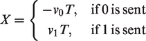
A binary communication system, shown in Figure 1, sends a 0 bit by transmitting a rectangular pulse of magnitude 

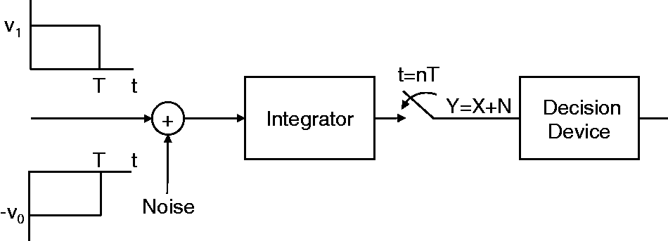
Binary signal detection.
The receiver uses the following decision rule, at the end of each T second interval, to decide which bit was transmitted during that interval:
If Y > k decide bit 1 was transmitted, else if Y < k decide bit 0 was transmitted, else if Y = k then decide randomly between bit 1 and 0 with equal probability.
In the above, k denotes the decision threshold. The goal is to design the “most reliable” receiver. In other words, what is the value of the optimal threshold k, denoted
Solution
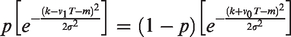
The probability of bit error at the receiver, Pe, is given by the total probability theorem

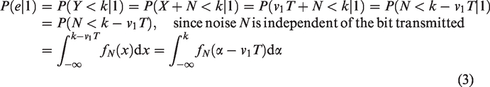
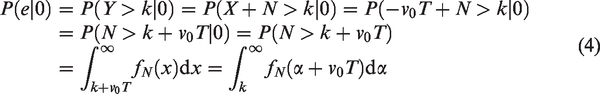
Substituting equations (3) and (4) into equation (2)


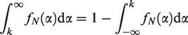
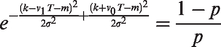
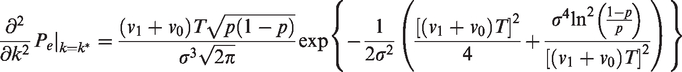
Note that Pe in equation (6) is a function of the decision threshold k. In order to find the optimum value of the threshold k, we need to differentiate equation (6) with respect to k and set it equal to 0 to find the critical point. Using the fundamental theorem of calculus and the following property of PDFs

Substituting equation (1) into above
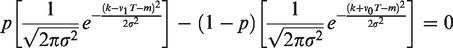
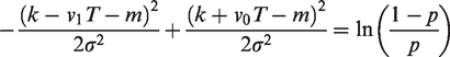
After some simplification
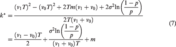
The optimal threshold given by equation (7) depends upon pulse amplitudes v0 and v1, pulse interval T, probability p of transmitting a bit 1, noise variance 
Differentiating equation (1) with respect to x yields
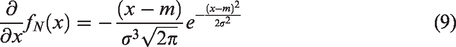
Substituting equation (9) into equation (8), we get
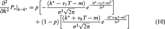
From equation (7), it follows that
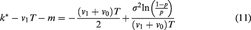
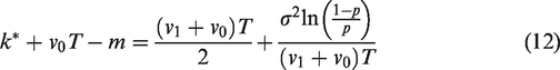
Substituting equations (11) and (12) into equation (10) and after some simplification, we get

Hence 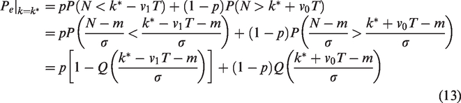
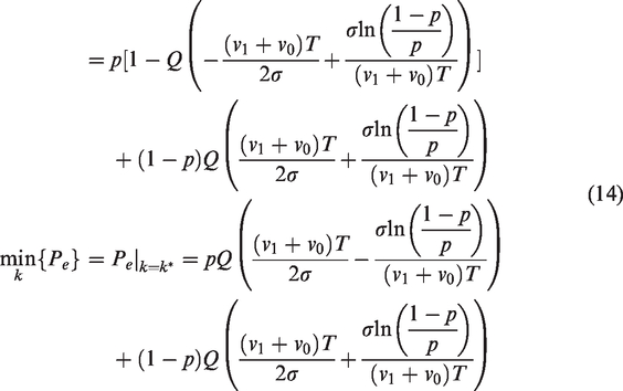
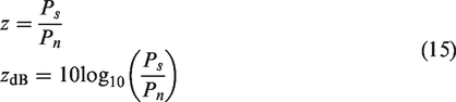
It is convenient to express the probability of bit error in equation (14) in terms of the signal-to-noise ratio (SNR). The SNR is defined as
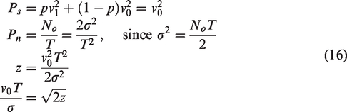
Substituting equation (16) and v1 = v0 in equation (14), we get
Equation (17) gives the minimum probability of error in equation (14) as a function of SNR for the antipodal signaling scheme. In the special case of equiprobable source bits (p = 1/2), antipodal signaling, and zero-mean Gaussian noise (m = 0), the optimal threshold 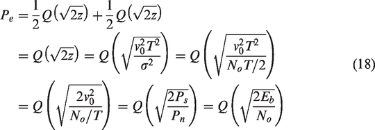
The reader would agree that the above mathematical analysis, though necessary, can make a student lose the sight of the forest for the trees. Often students are put off by involved mathematical analysis without a bigger picture in mind or alternative means of visualizing the concepts. This is especially true in an abstract course like probability where a lack of alternative means of accessing information can demotivate a student to pursue this subject. Simulations and visualization techniques can present information in a complementary way which significantly enhances the understanding of the student. In order to achieve the pedagogical objectives of Table 2, the following simulations were designed and presented to the students along with the mathematical analysis. It is to be noted that during the course of the semester, these simulations were presented side-by-side the mathematical analysis in an integrated manner.
Simulation
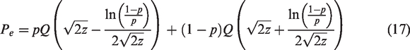
The system shown in Figure 1 was simulated using MATLAB®. A realization of the signal waveforms at different points along the system of Figure 1 is shown in Figure 2. Figure 2(a) shows the transmitted signal waveform corresponding to the bit sequence “01001.” Under the idealized conditions of no noise and channel distortion, the received signal at the input of the integrator in Figure 1 will be the same as the transmitted signal. However, due to the channel noise, the received signal is distorted. A realization of this distorted noisy received signal at the input of the integrator is shown in Figure 2(b). Figure 2(b) only shows one such realization, but as part of the simulation, multiple realizations of the received signal were presented to the students to illustrate the random effects of noise. Figure 2(c) shows the output of the integrator for a realization of the received signal corresponding to the bit sequence “01001.” By looking at Figure 2(c), the students were able to see how decoding errors occur randomly at the sampling instants in the receiver. For example, at T = 2 ms sampling instance, a decoding error occurs because the noise brings the sampled value under the optimal threshold of 0, even though a bit 1 was transmitted during the bit interval between 1 and 2 ms. On the other hand, the receiver decides correctly at the sampling instance of T = 3 ms. The simulation was repeated to show that transmitting the same bit sequence under exactly the same conditions may result in bit errors at different time instants due to the randomness of the noise; however, even this randomness follows certain mathematical laws which are the subject of the probability theory.
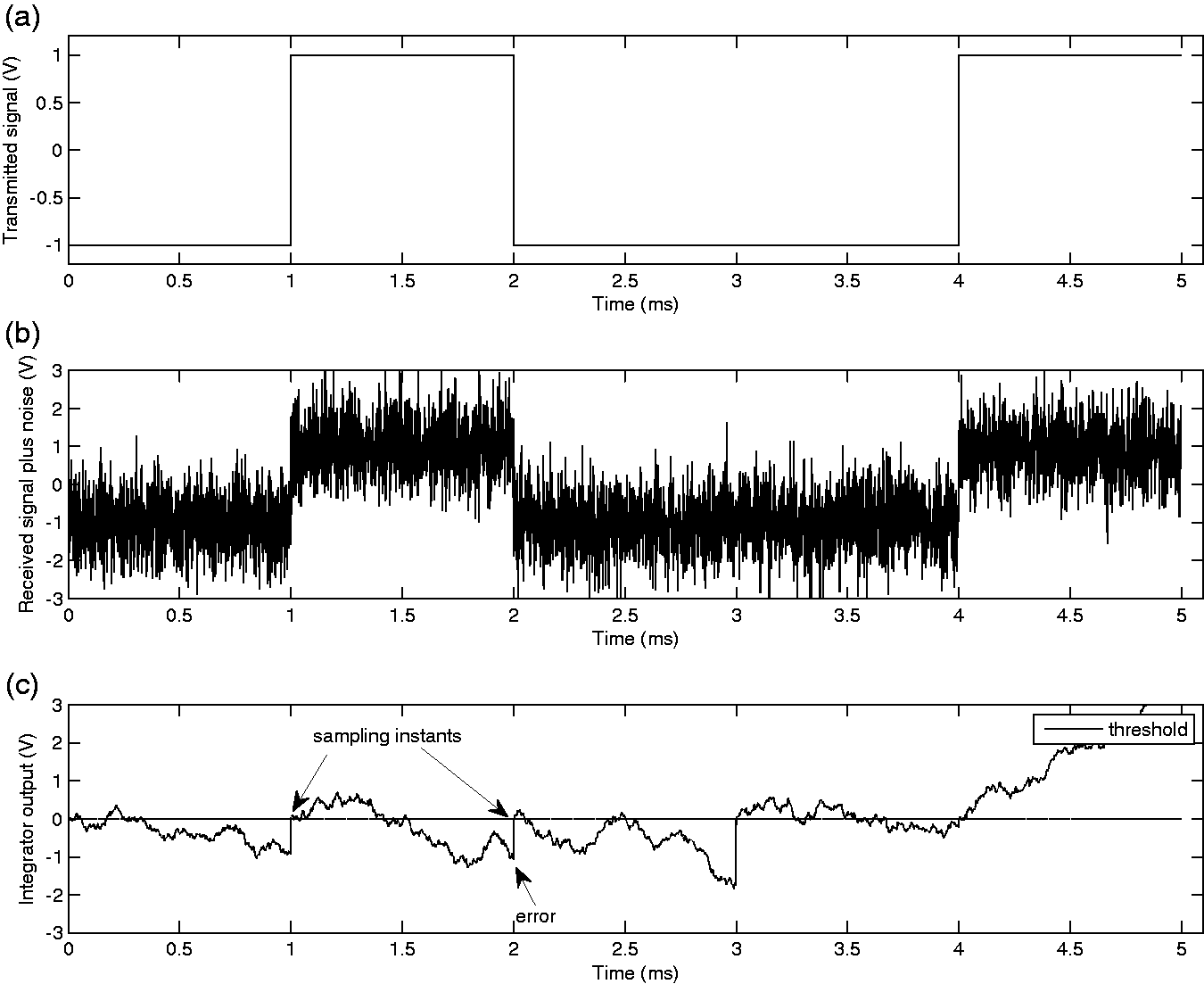
A realization of the signal waveforms for the system shown in Figure 1; v0 = 1 V, v1 = 1 V, T = 1 ms, p = 1/2, m = 0 mV, and
The students were able to interact with the simulation by changing different system parameters such as noise power, transmitted signal power, and transmitted bit sequence. This provided them a visual interpretation of the effects of signal and noise power on the bit errors. As a result, the students were better able to understand the role of uncertainty due to noise in the performance of a communication system.
An intuitive understanding of abstract probabilistic concepts such as random variable, random process, mean, variance, autocorrelation, power spectral density, stationarity, and ergodicity, can be developed by considering Figure 3 which shows five out of infinitely many possible realizations of the received signal at the integrator output. Each one of these waveforms occurs with a certain probability. The receiver has no a priori knowledge of which one of these waveforms is actually sent; if it did, there would be no point of transmitting any information. The collection or ensemble of these waveforms is called a random process, and each waveform is called a sample function. If we fix the time axis, then the ensemble of real numbers obtained constitutes a random variable. A random process is stationary if its statistics are time-invariant; in other words, they do not depend on the time origin. A random process is ergodic if its ensemble averages, across the sample functions, are equal to the time averages of a single sample function. For example, the mean of the process shown in Figure 3 is zero and consequently does not depend on the time instance. However, this process is not ergodic. To see this consider, a sample function consisting of all 1’s whose time average will not be equal to zero.
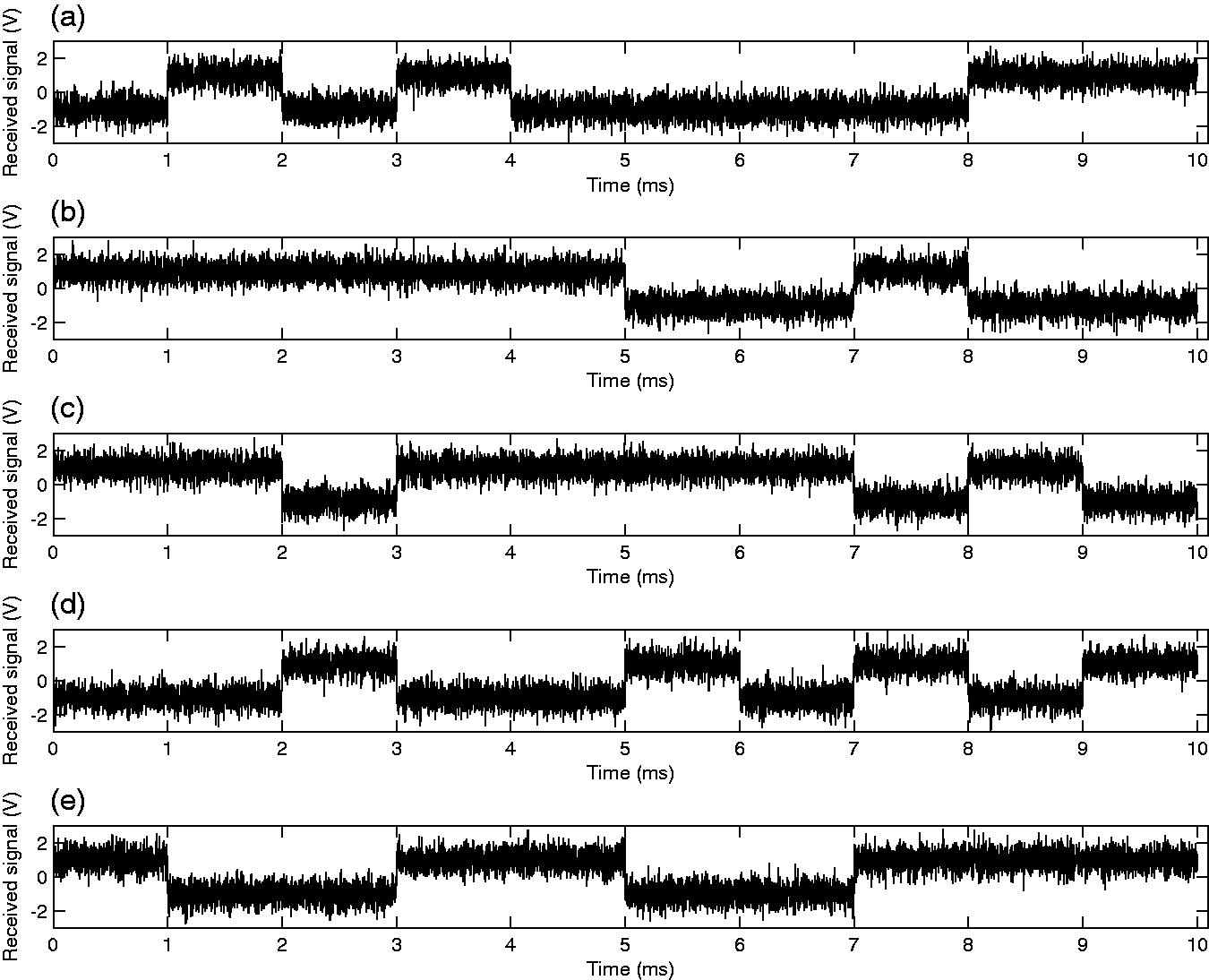
Multiple realizations of the received signal plus noise random process at the input of the integrator for the system shown in Figure 1; v0 = 1 V, v1 = 1 V, T = 1 ms, p = 1/2, m = 0 mV, and
An intuitive understanding of why an integrator is used in the receiver of Figure 1 can be garnered from Figure 2(c). As shown by the figure, the integrator smooths out the noise fluctuations while spreading the distance between the output of the two pulses v0 and v1 in the absence of noise. Another way of looking at this is to realize that an integrator acts as a lowpass filter and rejects the high-frequency component of noise that is outside the bandwidth of the transmitted pulse without loss of any information. In actuality, the integrator is the optimal filter for the transmitted signal pulses in the sense that it maximizes the output SNR ratio among the class of all LTI systems (matched filter), but this fact is left out for more advanced courses.
It is to be noted that a complete comprehension of the system in Figure 1 would require an understanding of random processes and the response of an LTI system to a wide-sense stationary random process, something that is covered toward the end of an introductory probability course. This is a common problem in using real-world engineering applications to introduce probabilistic concepts as these applications depend upon ideas introduced during different parts of the course. However, this constraint should not preclude application like these and associated simulations from being introduced to the students at an early stage of the course. For example, by using abstraction or information hiding, the information pertaining to the response of an LTI system to a wide-sense stationary process was abstracted out in “Problem statement” section. Later, during the course, when students were introduced to the response of an LTI system to a wide-sense stationary random process, then those aspects of this application and simulation were revealed to them.
In order to further illustrate the effects of different physical parameters on the performance of the system in Figure 1 in a hands-on and interactive manner, more interactive simulations were designed showing the sequence of sampled values at the output of the integrator. This particular visualization approach of showing the sequence of sampled values at the output of the integrator, sequence of random variables that constitute the decision statistic, provides a convenient way of observing the effects of different parameters on the performance of the system, thus revealing a deeper insight into the problem and developing probabilistic intuition. The performance of the system in Figure 1 is measured in terms of probability of bit error, Pe, also known as the BER. This is the likelihood of a bit being in error at the output of the decision device. The frequentist’s interpretation of this is the proportion of errors Ne in a large number of independent and identical transmissions N, i.e.,
Effect of noise variance
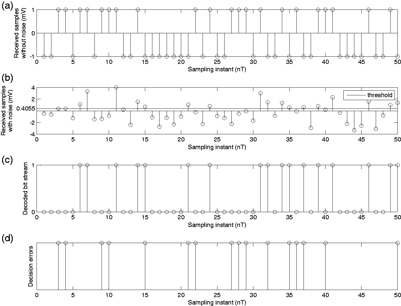
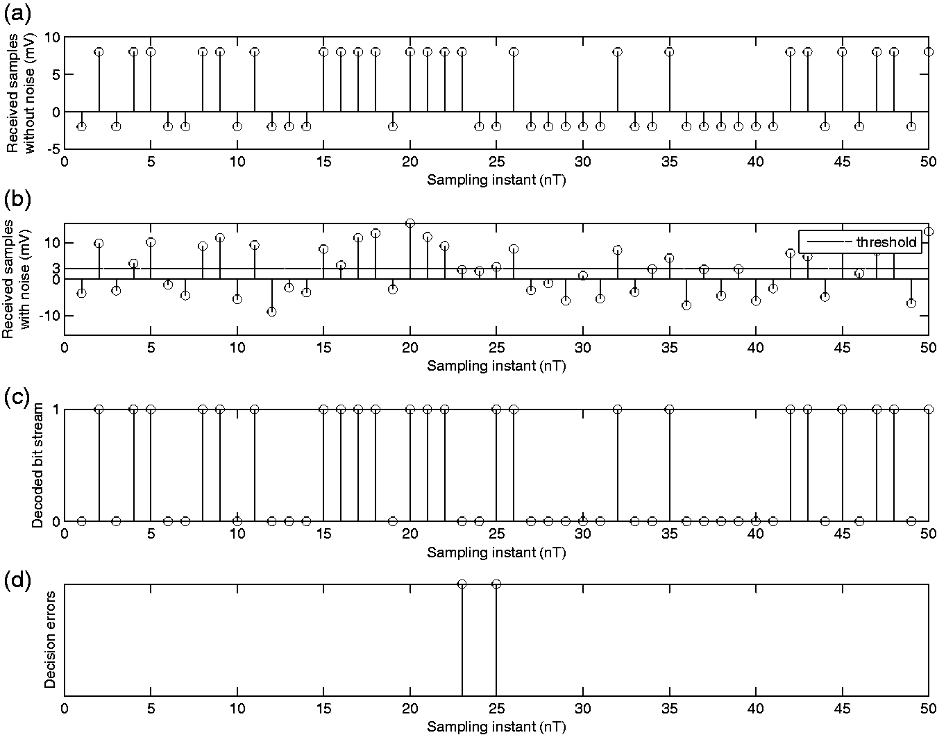
Figures 4 and 5 show the effect of noise variance on the probability of bit error of the system shown in Figure 1. Figure 4(a) shows a realization of the received sample values in the absence of noise at the output of the integrator; Figure 4(b) shows a realization of the received sample values with noise at the output of the integrator, i.e. the sequence of random variables Y that are fed into the decision device in Figure 1. The effect of noise perturbing the sample values corresponding to the transmitted signal is evident from this figure. The decision threshold of 0 is also shown in this figure. If the received sample is greater than the decision threshold, then the receiver decides in favor of bit 1; else if it is less than the threshold, the receiver decides in favor of bit 0. If the sample value is equal to the threshold, then the receiver decides between bit 1 and 0 with equal probability. Using this decision rule, the decoded bitstream is shown in Figure 4(c). Finally, the bits in error are displayed in Figure 4(d).
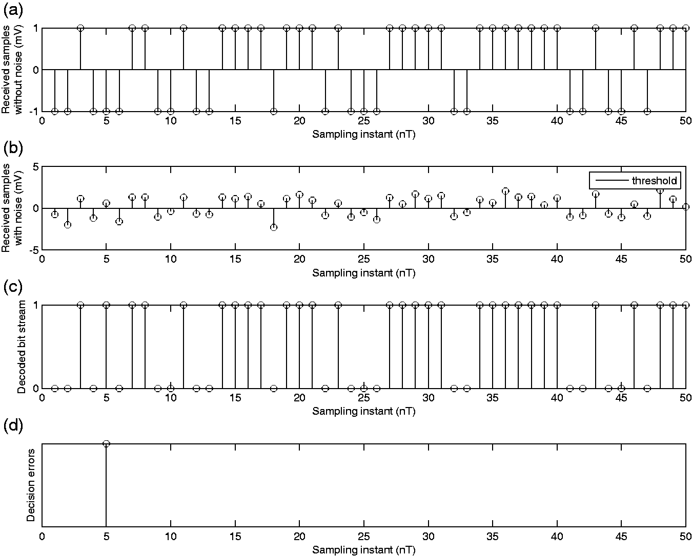
Effect of noise variance on the BER Pe of the system shown in Figure 1;
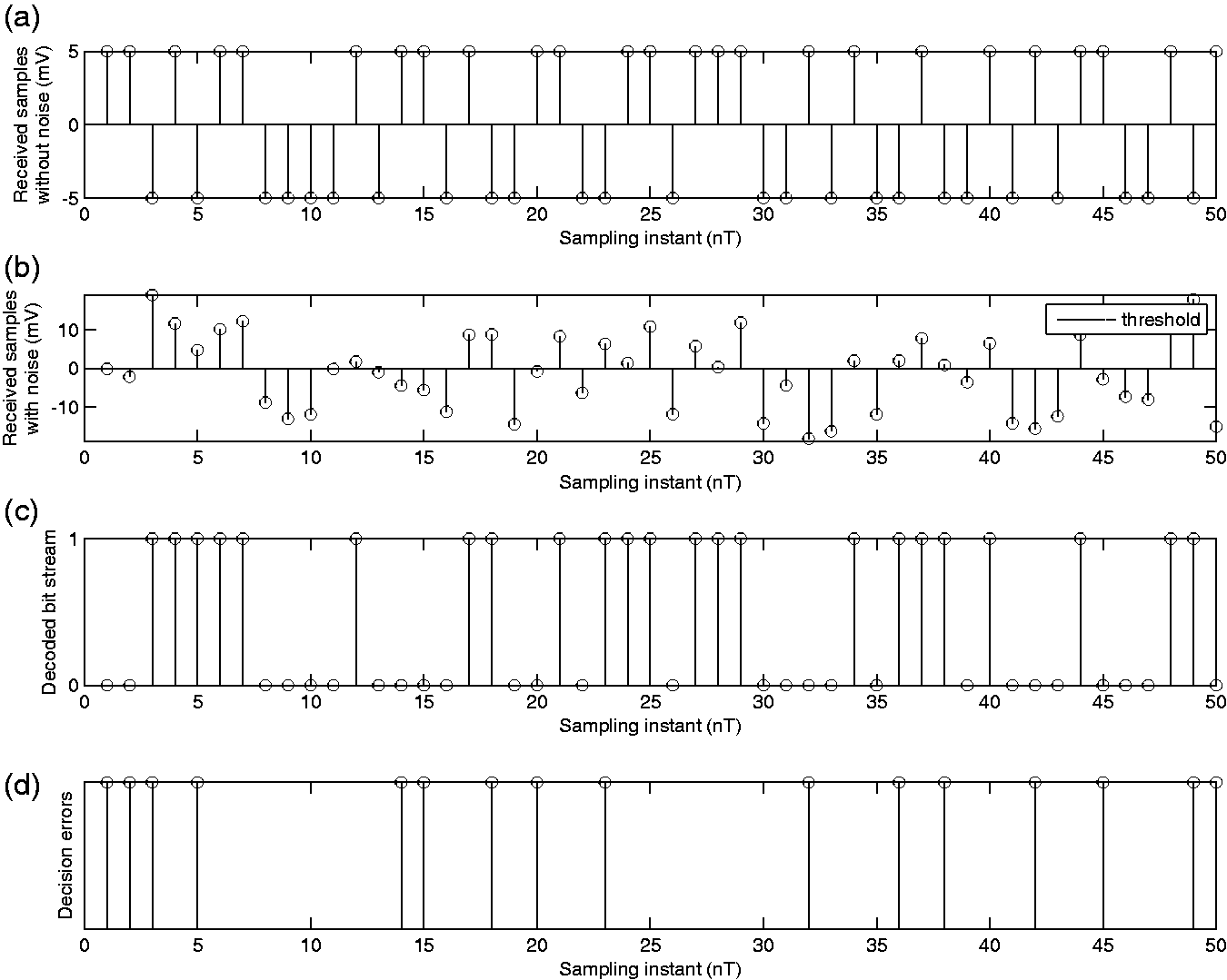
Effect of noise variance on the BER Pe of the system shown in Figure 1;
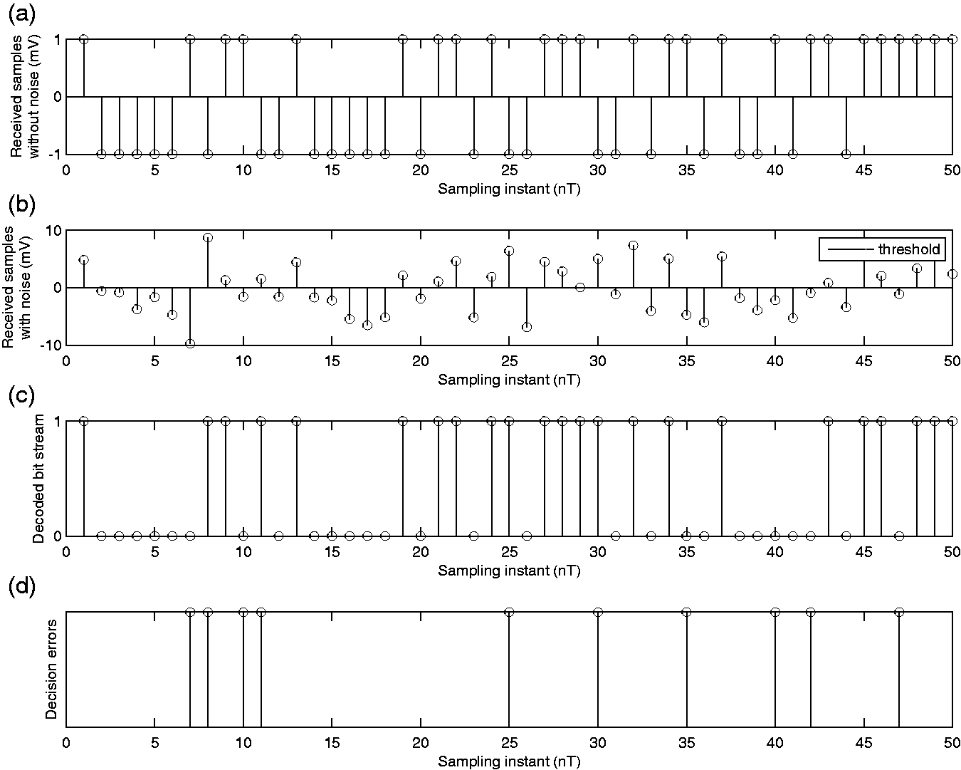
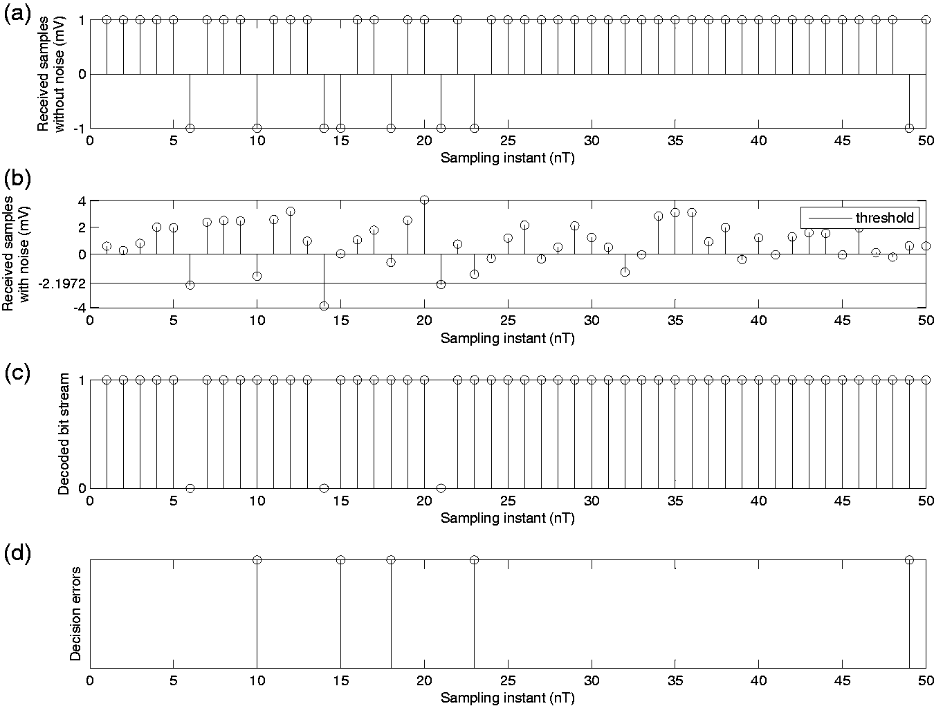
The simulation provides an interactive way of changing the noise variance and visualizing its effect on the received sample values and probability of bit error. Here, we present two sample figures, Figures 4 and 5, from the simulation. A comparison of these two figures will reveal the effect of noise variance on the probability of bit error. As noise variance is increased hundred folds from Figures 4 to 5, the number of bit errors increases. This is because variance is a measure of spread or dispersion around the mean, and an increase in noise variance results in larger fluctuations around the sample value X corresponding to the transmitted bit, hence resulting in more erroneous crossovers across the decision threshold. This phenomenon can easily be seen by comparing Figures 4(b) and 5(b). The resulting increase in the error rate is evident by comparing Figures 4(d) and 5(d). Often, concepts like mean and variance are presented only as mathematical formulae. By providing illustrative physical examples similar to these can really bring these abstract ideas home to the student.
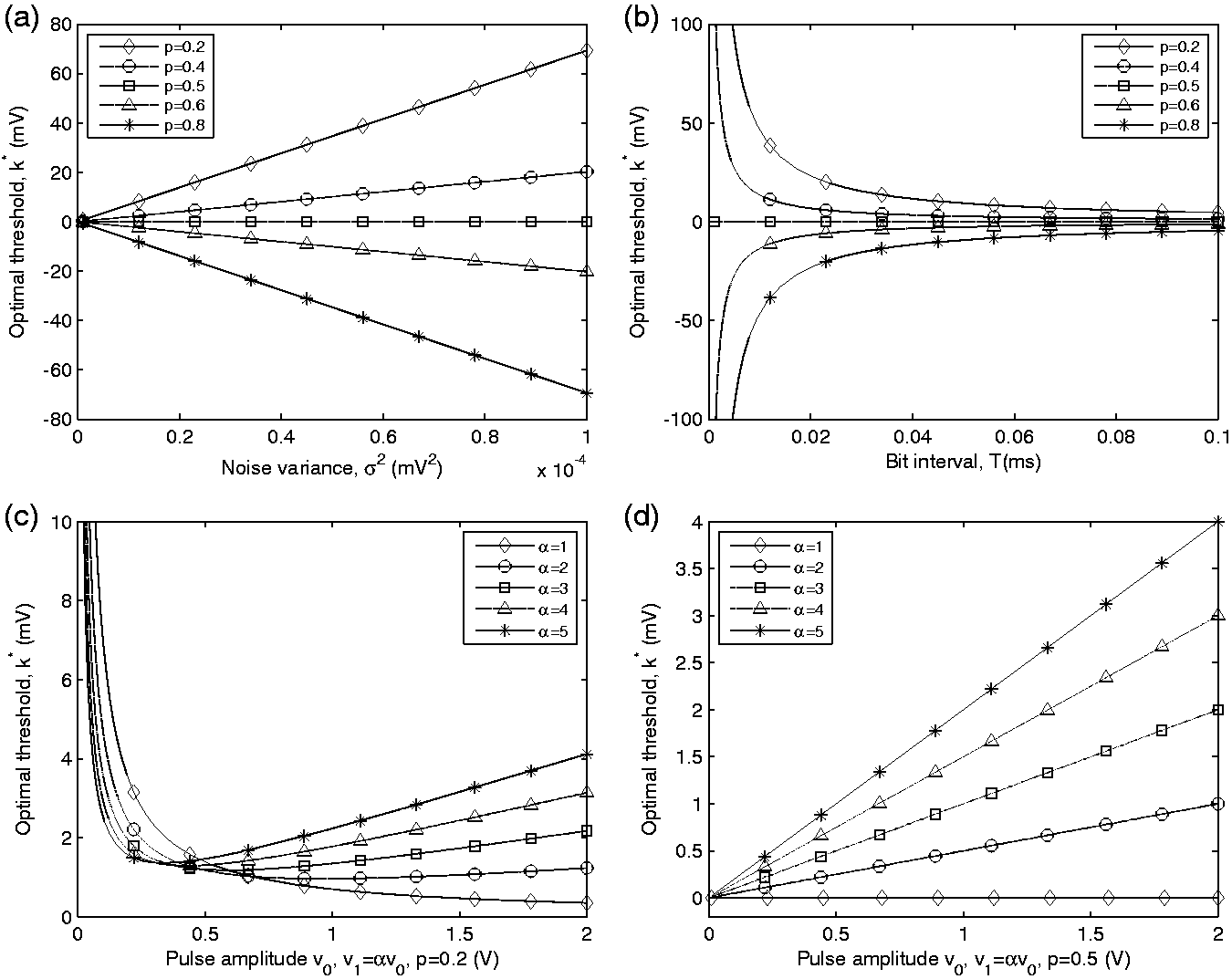
Figure 16(a) shows the behavior of the optimal decision threshold as a function of noise variance. We observe that the threshold value changes linearly with noise variance, where the slope of this linear dependence is positive for
Effect of transmitted bit probability
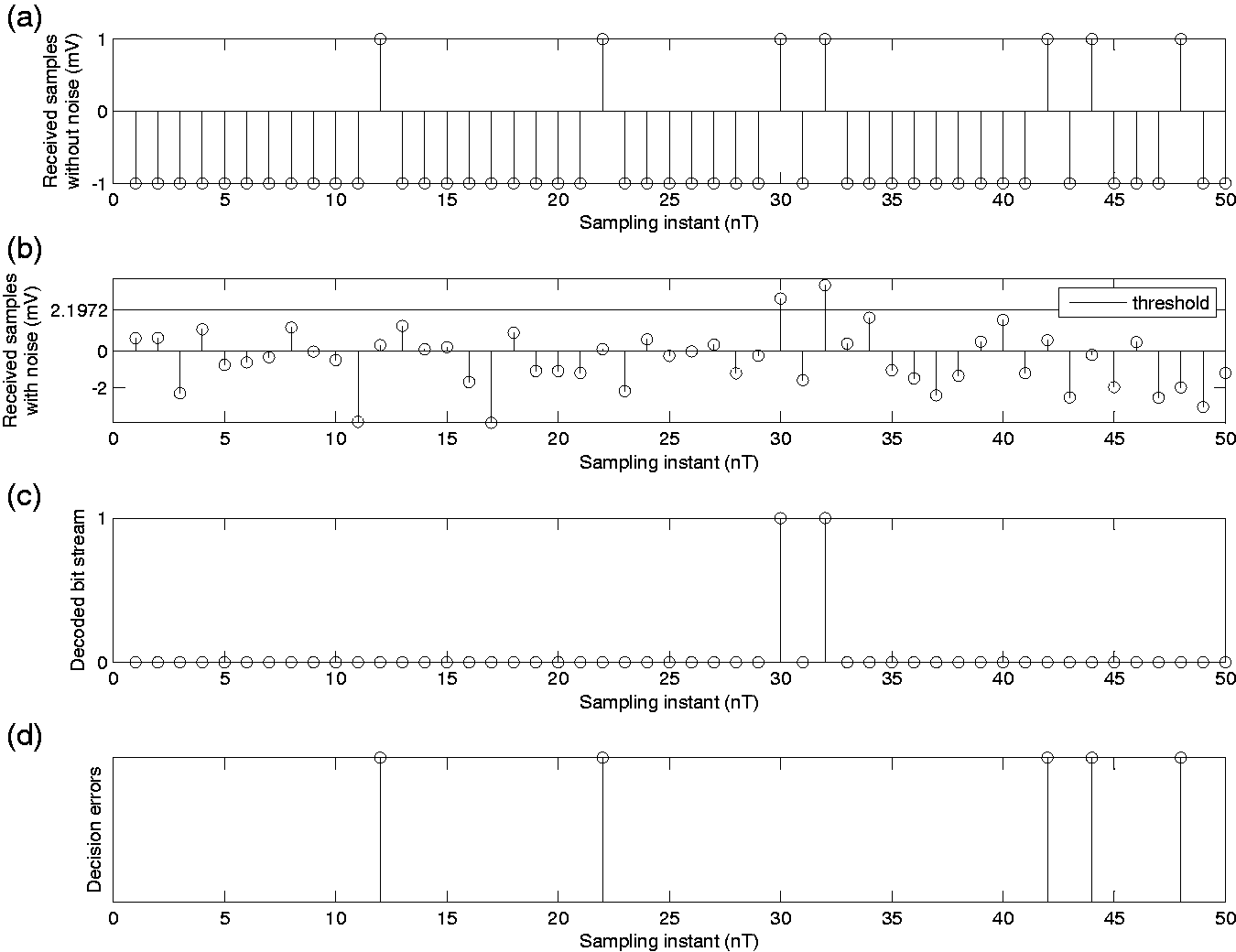
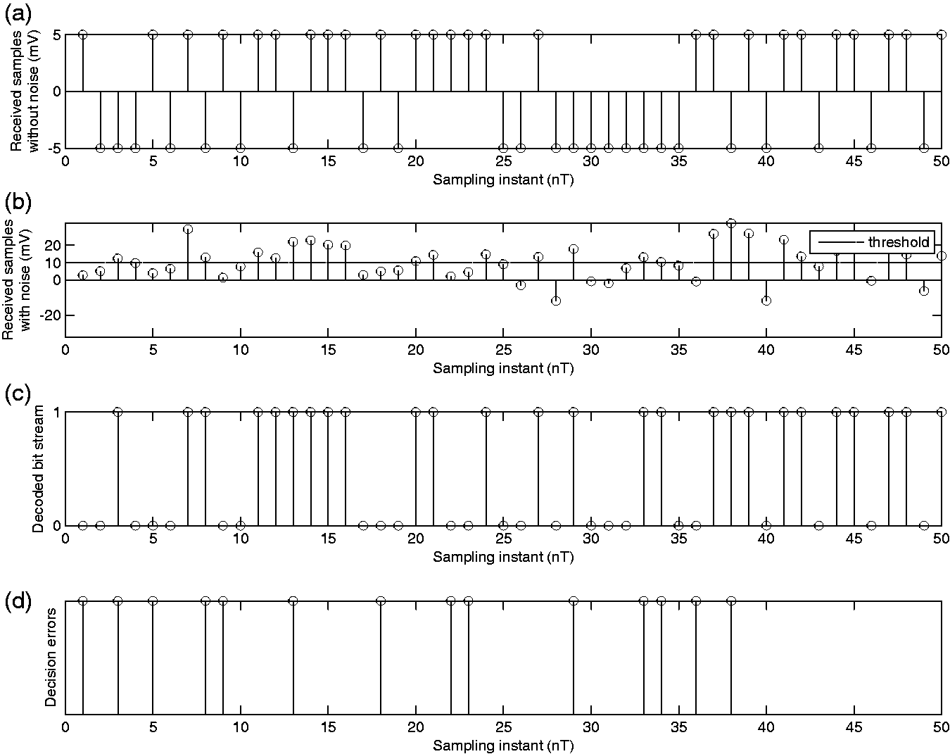
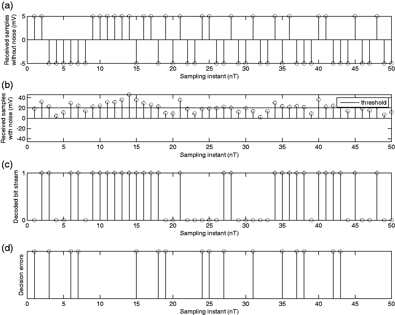
The effect of the probability of transmission of bit 1 on the optimal decision threshold and the probability of bit error is shown by Figures 6 to 8. Figures 6(b) and 7(b) show that as the likelihood of transmitting bit 1 decreases from 0.4 to 0.1, the optimal decision threshold increases from 0.4055 to 2.1972 mV, whereas the probability of bit error decreases from 0.2309 to 0.0908. The reason for the increase in the threshold is because when it is less likely that a 1 was transmitted, it is to the receiver’s advantage that it should err on the side of deciding a 0. This fact provides an intuitive understanding of the total probability theorem. The total probability of error according to the total probability theorem is given by

Effect of transmitted bit probability p on the optimal threshold
Effect of transmitted bit probability p on the optimal threshold
As p decreases, moving the threshold in the positive direction results in a larger value of
Effect of transmitted bit probability p on the optimal threshold
Figures 15(a) to (c) show the dependence of optimal decision threshold
Effect of transmitted signal amplitude
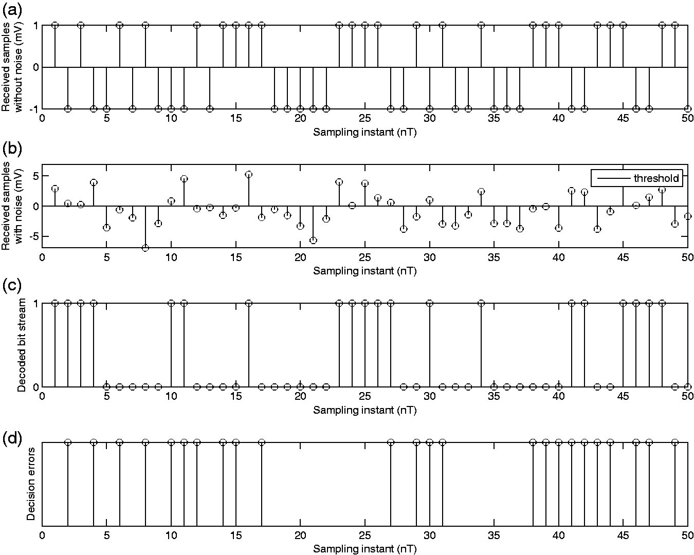
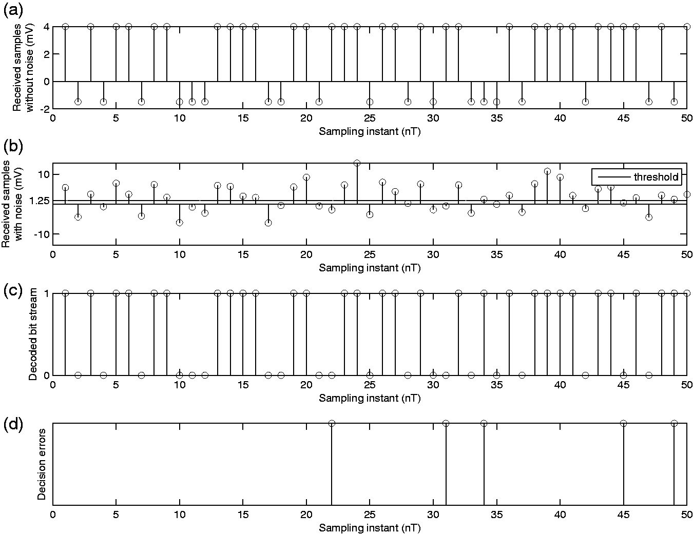
Figures 9 to 11 illustrate the effect of increasing the amplitude, and consequently power, of the transmitted pulses on the decision threshold and BER. A comparison of Figures 9(b), 10(b), and 11(b) would reveal that as the transmitted signal amplitudes increase asymmetrically, such that
Effect of transmitted signal amplitudes v0 and v1 on the optimal threshold
Effect of transmitted signal amplitudes v0 and v1 on the optimal threshold
Effect of transmitted signal amplitudes v0 and v1 on the optimal threshold
Figures 16(c) and (d) and 17 illustrate the effect of pulse amplitudes on the decision threshold. Figure 16(c) shows the dependence of decision threshold on pulse amplitudes for p = 0.2, i.e. when 0’s are more likely to be transmitted than 1’s. Under this condition, the threshold moves in the positive direction to reduce the overall rate of error; however, this shift in the positive direction increases with an increase in the pulse amplitudes under the constraint that
Similar behavior is observed in Figure 16(d) for the case when 0’s and 1’s are equally likely to be transmitted. As the magnitude of the pulses increases, under the constraint that
Figure 17 shows the dependence of the decision threshold on pulse amplitudes when 1’s are more likely to be transmitted than 0’s. Under this scenario, the threshold should shift in the negative direction due to the higher likelihood of transmitting a 1; however, the proportionately larger increase in the amplitude of v1 forces the threshold to move in the positive direction. The net effect of these conflicting objectives is illustrated by the curves in Figure 17.
Effect of noise mean
The effect of noise mean on the performance of the system can be understood from Figures 12 to 14. As the noise mean increases in the positive direction, the decision threshold also shifts in the positive direction by the same amount; however, the BER is unaffected. This can be explained by observing that the positive mean of noise shifts the random fluctuations in the received samples by an amount equal to the noise mean. Consequently, the likelihood of a bit error, given bit 0 was transmitted, becomes greater than the likelihood of error, given bit 1 was transmitted, if the threshold were to stay at 0. By moving the threshold in the positive direction, the total probability of error can be reduced when compared to the value obtained with a threshold of 0. The BER does not change in Figures 12 to 14 because by moving the decision threshold by an amount equal to the noise mean, in terms of performance, the system is equivalent to that when both noise mean and decision threshold are equal to 0.
Effect of noise mean m on the optimal threshold
Effect of noise mean m on the optimal threshold
Effect of noise mean m on the optimal threshold
Figure 15(d) shows that the optimal decision threshold linearly increases with noise mean. We also observe that for any
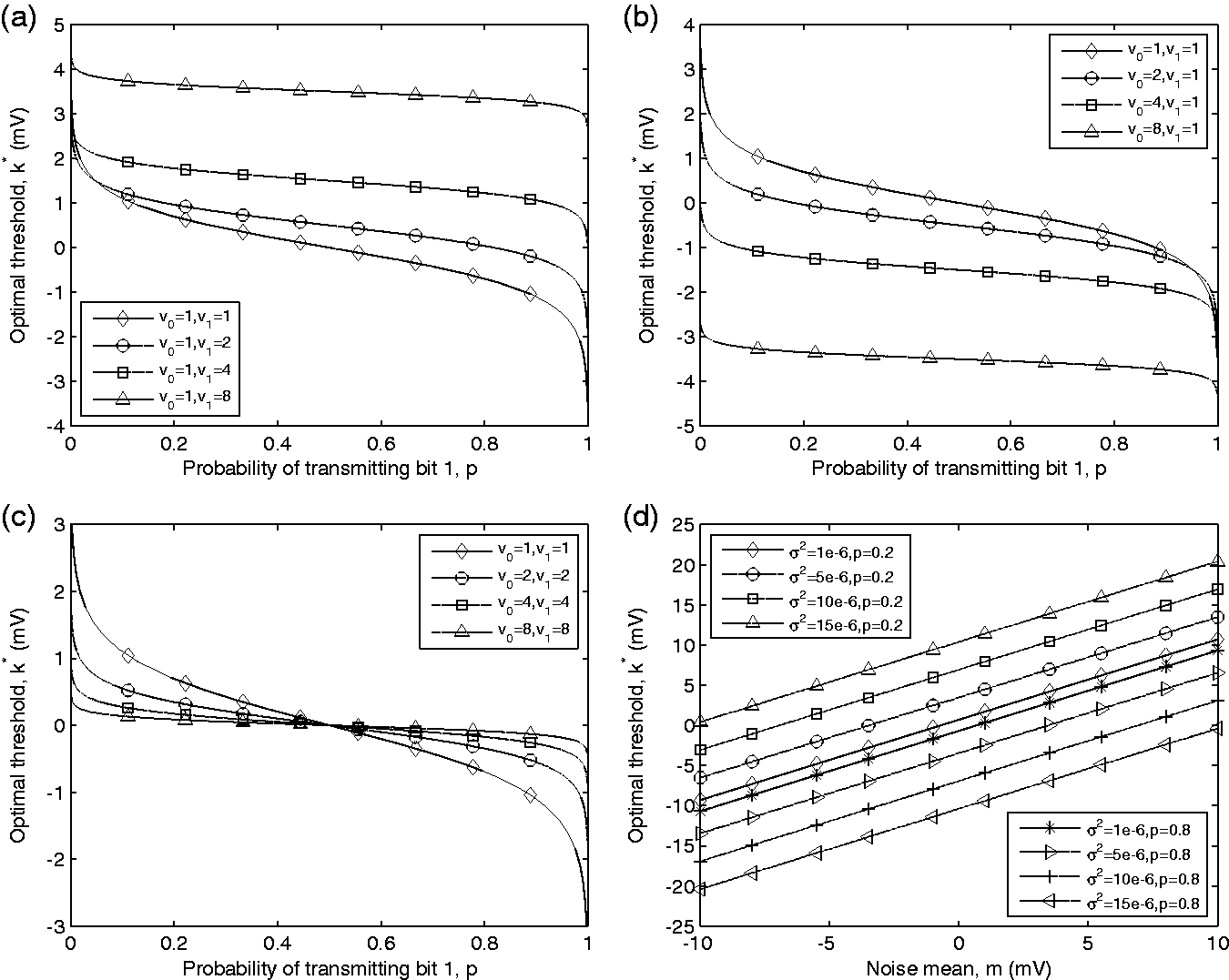
Effect of probability p of transmitting bit 1 on the optimal threshold
Effect of bit interval
Figure 16(b) shows the effect of the duration of transmitted pulses on the decision threshold. As the time duration of the pulses increases, their bandwidth decreases. This results in lesser noise power within the signal bandwidth perturbing the decision statistic. Note that because of the integrator, which acts as a lowpass filter, only the spectral component of the noise within the transmitted signal bandwidth has an impact on the performance of the system. Consequently, the net effect of an increase in the pulse duration is an increase in the SNR ratio of the decision statistic. At higher SNR values, the advantage of shifting the decision threshold away from zero diminishes, and hence the threshold curves get closer to zero as shown in Figure 16(b).
(a) Effect of noise variance
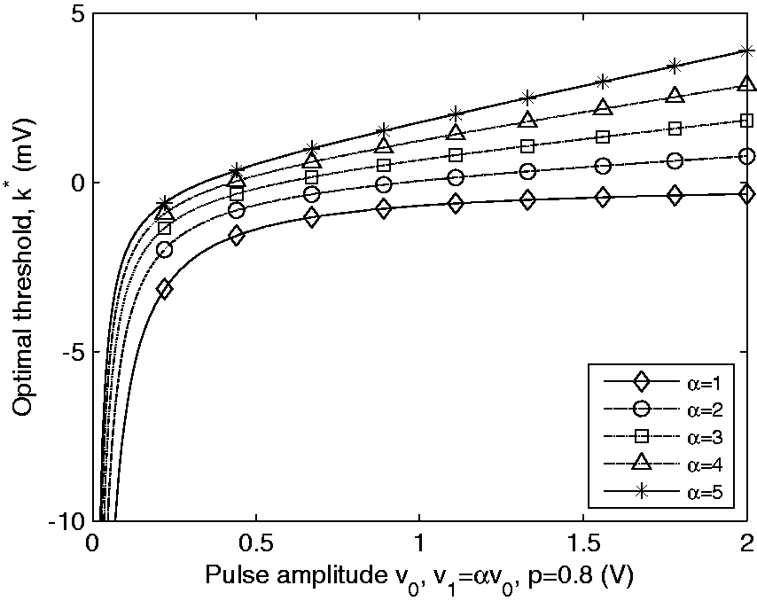
Effect of transmitted pulse amplitudes, v0 and v1, on the optimal threshold
Effect of SNR on bit error probability
The performance of the system in Figure 1 is measured in terms of the probability of bit error, Pe, which depends on the SNR ratio of the transmitted signals. The SNR is defined by equation (15), and the probability of bit error is given by equation (17), where z is the SNR, p is the probability of transmitting a bit 1, and Q(x) is the Q-function. In order to graphically show the dependence of Pe on SNR, Monte-Carlo simulations were performed to get the performance curves shown in Figure 18. Figure 18(a) shows the performance curves for
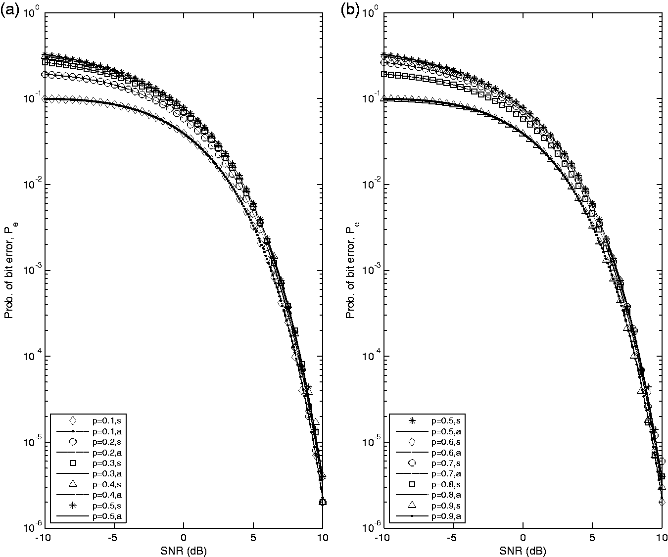
Effect of SNR ratio in dB on the probability of bit error, Pe (s: simulated; a: analytical); total number of iterations for Monte-Carlo simulations = 106. (a)
For each simulated value of Pe, 106 iterations of Monte-Carlo simulations were performed. Each simulated value of Pe is itself a random variable which is an estimate of the actual analytical Pe. How close the estimate is to the actual value is measured by its unbiasedness (mean of the estimate is equal to the actual value being estimated) and small variance as the number of iterations grows. The estimate used in the simulations satisfies these two criteria. To ensure that the standard deviation of the estimate is less than the probability that we are trying to estimate, a good rule of thumb is to have at least
The plots in Figure 18 show that the simulation results are in close agreement with the analytical results. The physical meaning of these curves can be discerned by considering the value of Pe at some point on the curve, for example, consider the point corresponding to SNR = 0 dB on the p = 0.5 curve. An SNR value of 0 dB corresponds to a signal power equal to that of the noise power. For this curve, the corresponding value of Pe is 0.0786, or in other words, approximately 7.865% of the bits will be in error for a sufficiently large number of independent bit transmissions.
Figure 18 shows the design tradeoff between transmitted signal power and the performance of the communication system measured in terms of the probability of bit error Pe. As expected, Pe decreases with an increase in SNR. In other words, the BER of the system can be brought down at the expense of putting more power into the transmitted signals. The simulations effectively highlight this design tradeoff which is an important aspect of any communication system.
The reader would also observe that in the low SNR region (SNR
The connection between the relative frequency of the frequentist’s approach and probability can be illustrated using this simulation. The link between the two is provided by the SLLN, which states that if X1, X2,…, Xn,… are a sequence of independent and identically distributed (IID) random variables with finite mean μ and finite variance, and let Mn be the sample mean given by

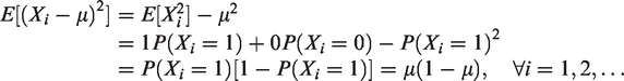
An intuitive understanding of this statement can be gained within the context of this simulation. Let X1, X2,…, Xn,…, be a sequence of IID Bernoulli random variables defined as

Since the mean and variance are finite, we can apply the SLLN to the sequence of IID random variables X1, X2,…, Xn,… The sample mean Mn in this context is given by

In other words, Mn in this context is the relative frequency or proportion of bit errors in the total number of IID iterations in a simulation run. Each nth iteration of a particular simulation run gives a fixed value for the random variable Mn. Stated in another way, each simulation run gives a sequence of real numbers, the values that the sequence of random variables M1, M2,…, Mn,… take. Notice that μ in this context is the actual probability of bit error Pe which we are trying to estimate using simulation. The SLLN provides a statement of the convergence of the relative frequency of bit errors to the actual probability of bit errors. What this convergence means is that if we run the simulation experiment multiple times for a sufficiently large number of iterations and then consider the set of those simulation runs in which the sequence of real numbers Mn converges to Pe, then this set is a certain event. In other words, the probability of obtaining an outcome from this event is 1. Equivalently, the probability of a simulation run in which the sequence Mn will not converge to Pe is zero. This type of convergence, when SLLN holds in physical systems, is known as statistical regularity, and it provides strong validation for using the relative frequency as an estimate of the actual probability in physical engineering systems.
Figures 19 and 20 show multiple outputs of the simulation runs illustrating the convergence of the relative frequency of bit errors Mn to Pe as a function of n, the number of iterations in a simulation run. This provides a visual interpretation of the SLLN. The simulation and associated plots in Figures 19 and 20 can also be used to clear the confusion surrounding the distinction between weak law of large numbers (WLLN) and SLLN. The WLLN is a statement of convergence in probability, as opposed to SLLN which is a statement of almost sure convergence. The WLLN is stated as follows: if X1, X2,…, Xn,…, are a sequence of IID random variables with finite mean μ, and let Mn be the sample mean given by
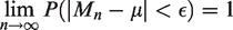
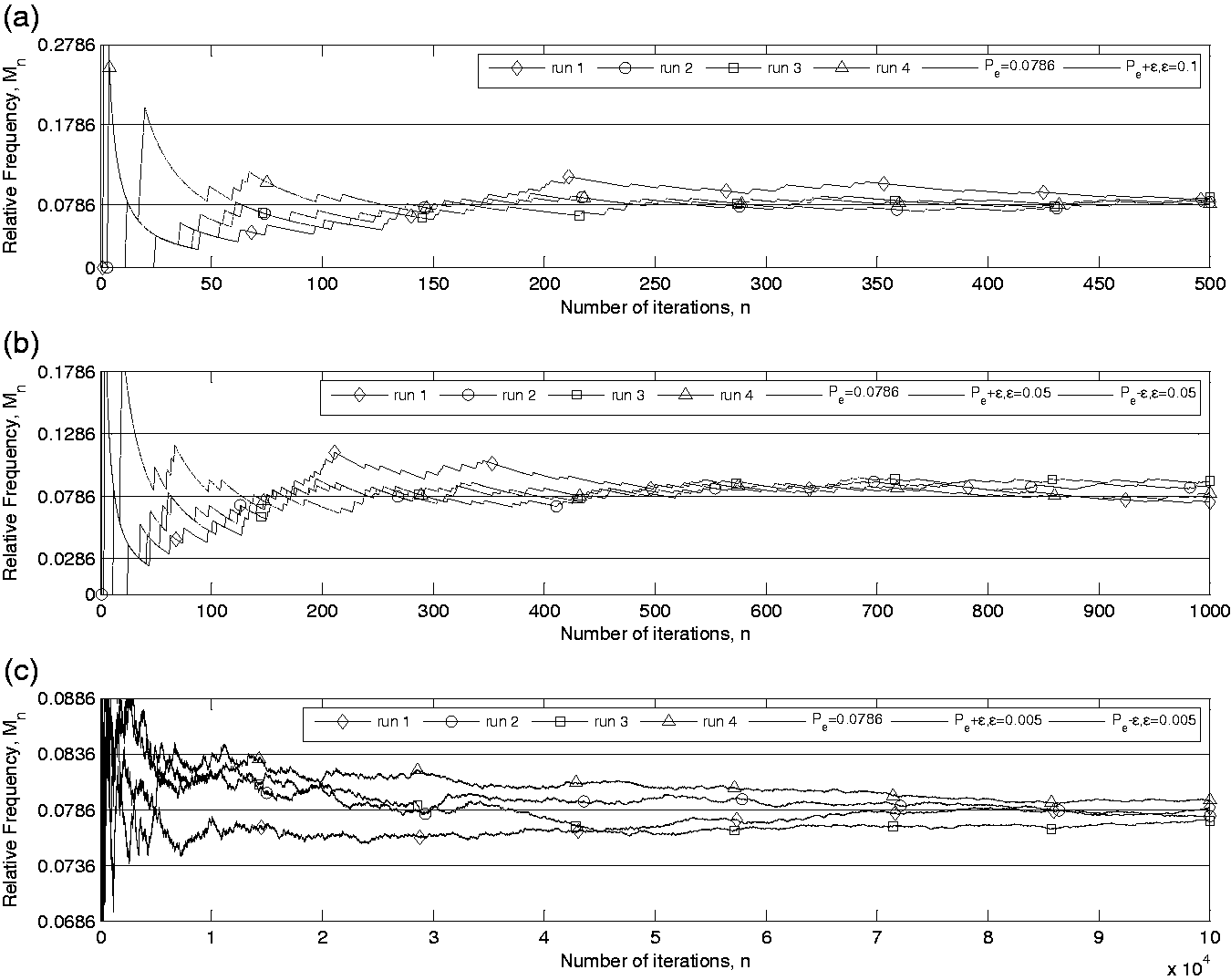
Illustration of the strong law of large numbers showing the convergence of simulated relative frequency to the analytical probability of bit error, p = 0.5, SNR = 0 dB,
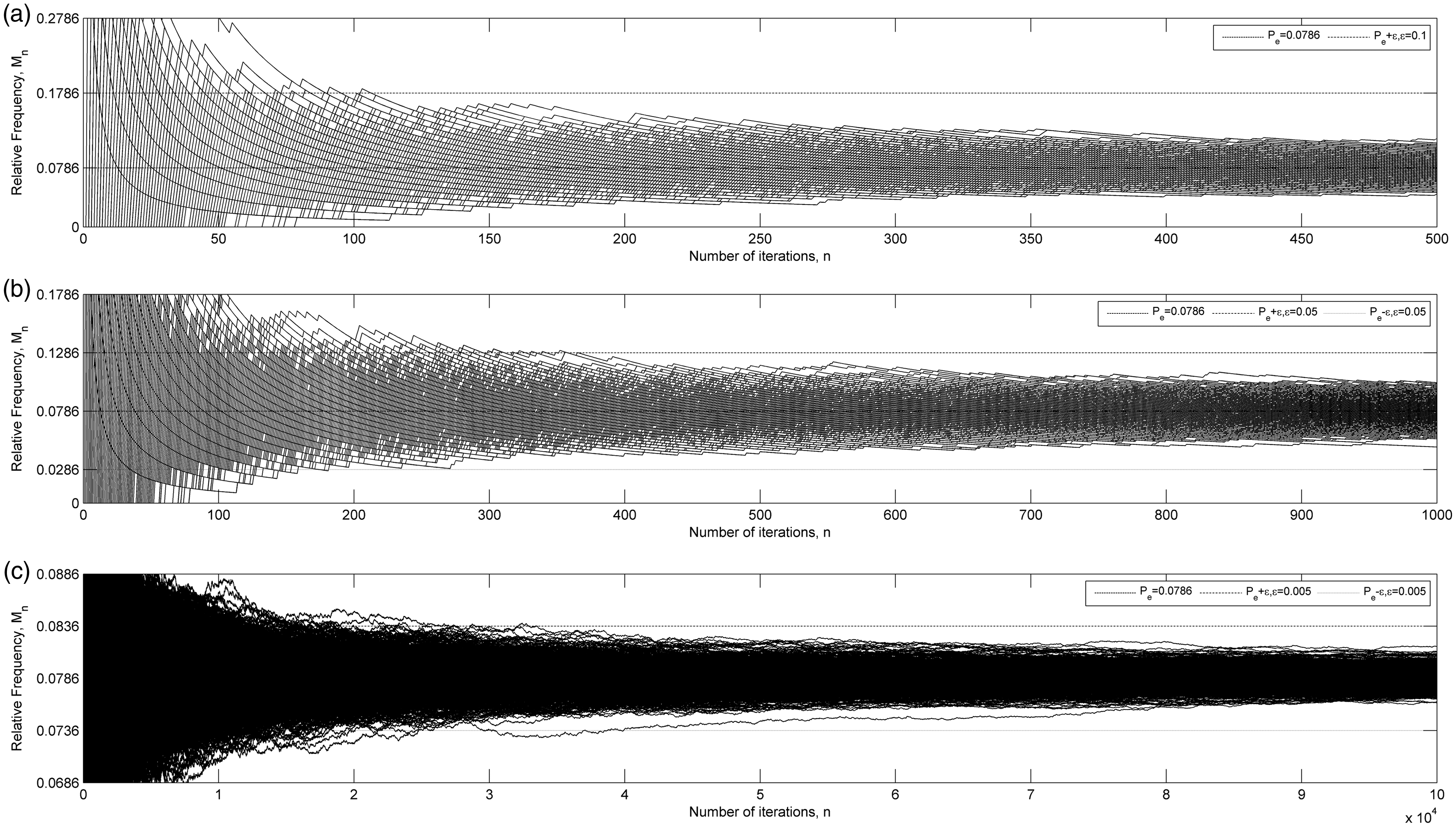
Illustration of the strong law of large numbers showing the convergence of simulated relative frequency to analytical probability of bit error, 1000 runs, p = 0.5, SNR = 0 dB,
Comparing the definitions of SLLN and WLLN, it is hard to get an intuitive understanding of the difference between them. However, by using the simulation plots in Figures 19 and 20, one can clarify this difference. Under WLLN, with non-zero probability, although very small and decreasing with large n, it is quite possible that at least one of the simulation run will go outside the ϵ distance from μ. Whereas, SLLN says that if we wait long enough, then all infinite sequences that occur with non-zero probability will eventually get inside the ϵ distance from μ and will stay within this distance for any arbitrary positive value of ϵ. Figure 20 shows that all thousand sequences eventually get within ϵ distance from μ and then stay within that band. Using this example, we emphasize again the role of simulations in clarifying abstract probabilistic concepts and correcting erroneous intuition.
Efficacy studies
In order to measure the efficacy of the proposed intuitive, application-based, simulation-driven approach to teaching probability, henceforth referred to as the intervention, a randomized experimental design was utilized. Since this particular course is taught at Purdue University Northwest, a smaller regional campus of Purdue University system, where the average class size for this course is around 10 students, a perfect randomized experimental design was not possible. Nevertheless, the experimental design was constructed to be as close as possible to a completely randomized design within the constraints of the course offering at a campus with small class sizes. Considering the shortcomings of the quantitative statistical tests due to small sample size, we also provide qualitative data from a student survey utilizing 5-point Likert-type scale and essay-based student responses to support the evidence for the efficacy of the proposed pedagogical approach. In addition, the quantitative statistical tests that we employ are the ones recommended for small sample sizes.
As shown below, the data collected from this study provides sufficient evidence, even if the findings are tempered due to the small sample size, for the efficacy of the intervention.
Experimental design
The experimental design consisted of two “randomly” assigned groups. Group 1, the treatment group, consisted of 13 junior-year ECE students who took Probabilistic Methods in Electrical and Computer Engineering (ECE 302) in the spring 2016 semester. Group 2, the control group, consisted of 10 junior-year ECE students who took ECE 302 in the spring 2015 semester. Due to small class sizes and lack of multiple sections, it was not possible to randomly assign subjects to two different groups during the same semester. Nevertheless, the effect of extraneous factors and bias was minimized by keeping the design of the two courses very similar except for the intervention. For instance, the course was taught by the same instructor to both groups using the same textbook, lectures, grading weights , course policy, and difficulty-level of homework, quizzes, and exams. The baseline competency of the two groups was comparable based on their performance in previous courses and the university selection process. The instructor also ensured that homework, quizzes, and exams were of comparable difficulty level throughout the course of the semester for the two groups.
Results
The independent variable was the proposed intuitive, application-based, simulation-driven approach to teaching probability, whereas the dependent variable was the total course score (out of 100%) of each student. The research question being investigated was whether the proposed intuitive, application-based, simulation-driven approach to teaching probability has a significant positive impact on students’ scores? In order to choose an appropriate statistical test to investigate this question, first, the data from each group were checked for normality. Due to the small sample size, Shapiro–Wilk 25 and Anderson–Darling 26 tests for normality were used with the null hypothesis that the sample is normal with unspecified mean and variance. The Shapiro–Wilk test failed to reject the null hypothesis for the treatment group at 5% significance level with a p-value p = 0.1883 and test statistic (non-normalized) W = 0.9159. The Anderson–Darling test also failed to reject the null hypothesis for the treatment group at 5% significance level with a p-value p = 0.1530, test statistic adstat = 0.5229, and critical value cv = 0.7024.
For the control group, the Shapiro–Wilk test failed to reject the null hypothesis at 5% significance level with a p-value p = 0.3439 and test statistic (non-normalized) W = 0.9247. Likewise, the Anderson–Darling test failed to reject the null hypothesis for the control group at 5% significance level with a p-value p = 0.4412, test statistic adstat = 0.3391, and critical value cv = 0.6857.
Based on the results of the normality tests, a two-sample t-test 27 was employed to test the null hypothesis that the student scores in the treatment and control groups came from independent random samples from normal distributions with equal means and unknown and unequal variances, and the alternative hypothesis that the data in treatment and control groups came from populations with unequal means.
The test rejected the null hypothesis at 5% significance level with p-value p = 0.0018, 95% confidence interval for the difference in population mean of the treatment group and the control group
Even though the normality tests failed to reject the normality null hypothesis, due to the small sample size and the fact that the median may also reveal valuable information about the populations, the Wilcoxon rank-sum test (equivalent to Mann–Whitney U test) 28 was also employed with the null hypothesis that student scores in treatment and control groups are independent samples from continuous distributions with equal medians. The Wilcoxon rank-sum test rejected the null hypothesis at a significance level of 5% with p-value p = 0.0026, rank-sum test statistic ranksum = 205, and z-statistic zval = 3.0078. To test the hypothesis of an increase in the population median of the treatment group, we used a left-sided Wilcoxon rank-sum test with the null hypothesis that student scores in treatment and control groups are independent samples from continuous distributions with the median of treatment group population less than the median of the control group population. The left-sided Wilcoxon rank-sum test rejected the null hypothesis at a significance level of 5% with p-value = 0.0013, rank-sum test statistic ranksum = 205, and z-statistic zval = 3.0078. The results of these non-parametric tests provide further evidence of the efficacy of the proposed intervention.
Student survey data
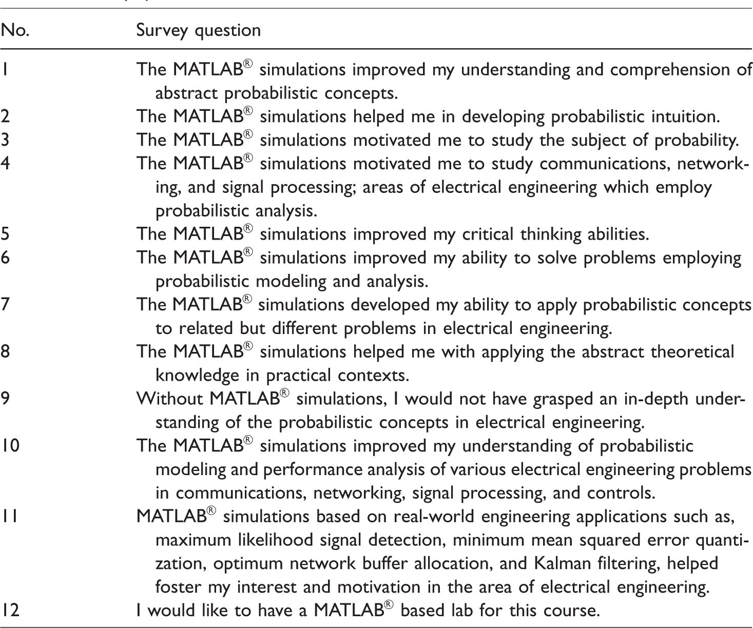
In addition to the quantitative data presented in “Results” section in support of the evidence for the efficacy of the proposed pedagogical technique, qualitative data from a survey utilizing 5-point Likert-type scale and essay-based student responses were also collected. The respondents for this survey were the same students from the treatment group mentioned in the “Experimental design” section. The survey was conducted online at the end of the semester with the students’ responses kept anonymous. Nine students provided their feedback through this survey. Table 3 lists the questions in the survey, and Figure 21 shows the results of the survey in terms of the frequency distribution of responses to each question on the survey. The survey explicitly mentioned that the term “MATLAB® simulations” in the context of the survey was used to describe the intuitive, application, and simulation-driven pedagogical teaching technique employed in teaching probability during the course of that semester. The results of this survey provide further qualitative evidence for the efficacy of the proposed pedagogical technique. In particular, 88.89% of the students either agreed or strongly agreed that the proposed pedagogical technique improved their understanding and comprehension of abstract probabilistic concepts and helped them in developing probabilistic intuition. About 77.78% of the students either agreed or strongly agreed that the pedagogical technique helped them in applying abstract probabilistic knowledge in practical contexts. The same percentage of students either agreed or strongly agreed that without the pedagogical technique, they would not have been able to grasp an in-depth understanding of the probabilistic concepts in ECE. On the other hand, the survey reveals that the proposed pedagogical techniques had a relatively less impact on motivating students to study probability. One of the remarkable results from this survey is that 88.89% of students either agreed or strongly agreed that they would like to have either a MATLAB®-based lab for this course or a significant portion of the course dedicated to simulation projects as traditionally a lab is not offered along with a probability course.
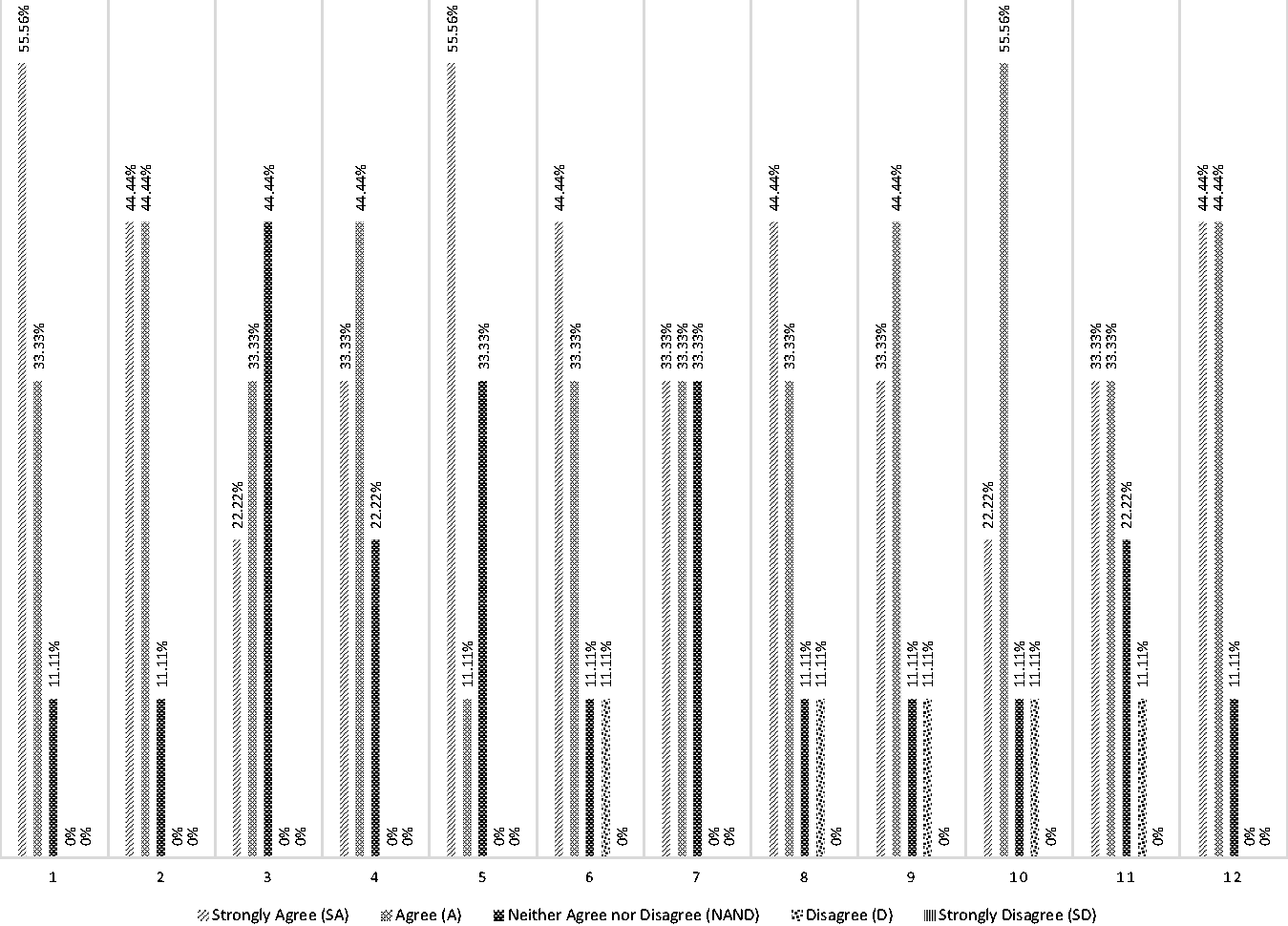
Frequency distribution of survey questions. Total number of survey respondents = 9.
Survey questions.
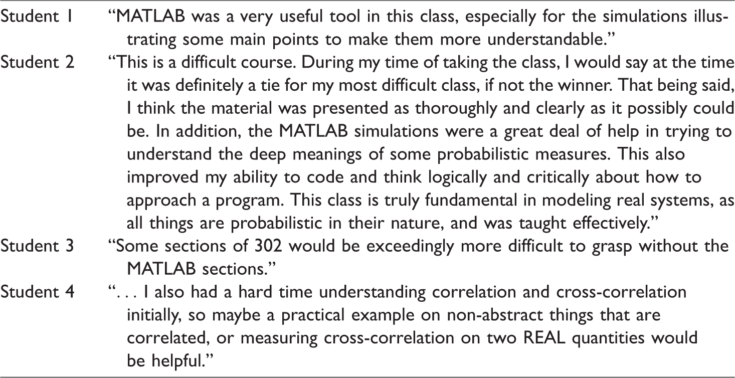
Some of the students’ comments from this survey are also presented in Table 4. They again highlight the importance of the proposed pedagogical technique in helping students develop probabilistic intuition and a deeper understanding of this esoteric subject.
Students’ comments.
Conclusion and future work
Probability and random processes, an important prerequisite for areas of electrical engineering such as communications, controls, signal processing, and networking, is generally considered a conceptually difficult and unintuitive subject by ECE undergraduates. 1 There are numerous reasons for the difficulty encountered by the students while learning this subject. First, due to our physical scale, how we have evolved, and how we observe the physical world with our naked eye, our brains are not wired to intuitively understand the probabilistic phenomena.3,4 For a long time, this subject has been taught in a very abstract manner with more emphasis on theory than on applications. Modern simulation and visualization tools such as MATLAB® are not often utilized to provide an alternative way of grasping this abstract subject. This paper presents an intuitive, application-based, simulation-driven pedagogical approach to teaching probability and random processes to ECE undergraduates. Some of the highlights of the proposed pedagogical approach entail introducing abstract probabilistic concepts using real-world applications of probability in ECE; extensive, tightly integrated, interactive MATLAB® simulations to build probabilistic intuition; use of relative frequency approach in simulations to complement the axiomatic approach; and modeling and analysis of optimal engineering systems design problems in the presence of uncertainty highlighting the design tradeoffs and their impact on the system performance. The proposed pedagogical approach was implemented during the course of a semester, and data were collected to ascertain the efficacy of this approach by comparing the performance of the treatment group with a control group. The statistical tests employed to measure the efficacy of this approach provide sufficient evidence toward the effectiveness of this approach. In addition, the student survey data provide another validation of the effectiveness of the proposed pedagogical technique. In the future, we intend to extend the proposed pedagogical technique to other courses in the ECE curriculum and measure its efficacy with a larger sample size.
Footnotes
Author's Note
Waseem Sheikh is now affiliated with the CSET Department, Oregon Institute of Technology, 3201 Campus Dr, Klamath Falls, OR 97601, USA. Email: waseem.sheikh@oit.edu
Declaration of Conflicting Interests
The author declared no potential conflicts of interest with respect to the research, authorship, and/or publication of this article.
Funding
The author received no financial support for the research, authorship, and/or publication of this article.