Sage Journals: Discover world-class research

Abstract

According to The Spirit Level, inequality is bad for everyone—including people with higher incomes. That conclusion is evident also in research exploring the impact of inequality on status anxiety. But existing research on this topic is cross-sectional (and gives too much weight to statistical significance). I construct a longitudinal analysis to explore whether status anxiety increases with inequality, especially among higher earners. I use country-level averages of status anxiety for this purpose and ignore individual-level control variables, on the grounds that they are not antecedents of the focal independent variable, inequality. In contrast to previous research, I find that increases in inequality lead to lower levels of status anxiety for higher earners. People at the top appear to benefit from inequality in this sense—a finding that runs against the idea that inequality is bad for everyone.

Keywords

Control variables Europe inequality longitudinal analysis status anxiety

Introduction

Is inequality bad for people at the top? The Spirit Level: Why Equality Is Better for Everyone (Wilkinson and Pickett, 2010) offers a strong version of this argument: already in the subtitle we learn that equality is better not just for lower earners but indeed for “everyone.” That formulation is perhaps hyperbolic,¹ but it is not far from the more nuanced position they take in their text: “The truth is that the vast majority of the population is harmed by greater inequality” (Wilkinson and Pickett, 2010: 176, emphasis added). We see the same perspective in their later work, The Inner Level: How More Equal Societies ... Improve Everyone’s Well-being (Wilkinson and Pickett, 2019). In the earlier work, the focus is on “objective” forms of well-being, including health measures such as life expectancy. In The Inner Level, the focus is on “subjective” forms of well-being, including status anxiety—and here as well the negative impacts of inequality are not felt only by lower earners: “Bigger income differences ... increase everyone’s social evaluation anxieties,” indicating “across all income groups ... [an] increase in stress throughout the populations of more unequal countries” (Wilkinson and Pickett, 2019: 34–35).

The idea that inequality harms wealthier people is a highly attractive position. In an early commentary on The Spirit Level (henceforth SL), Mills (2012) highlighted the essential implication: if even the wealthy would benefit from greater equality, then an egalitarian political project can proceed in part by helping the wealthy learn what is good for them. More conventionally, an egalitarian project entails conflict: to improve the lives of people at the bottom, we have to ask (or compel) people at the top to make do with less. The SL performs a disappearing act on this form of conflict: the “vast majority” will benefit from more equality. In effect, there is no conflict; all that is required is to demonstrate (especially to the wealthy) that this proposition is true.

Is there empirical support for the idea that even higher earners suffer from living in more unequal societies? This article evaluates existing research on this topic, giving attention to key methodological issues in ways indicating that the empirical support for this proposition has some significant vulnerabilities. The focus here is on the consequences of inequality for status anxiety—a key psychological mechanism for the impact of inequality on health outcomes (Wilkinson and Pickett, 2010, drawing, for example, on Marmot et al., 1978, 1991) and an important aspect of people’s well-being also in a subjective sense. Two issues are especially salient: (1) the studies on which Wilkinson and Pickett rely are cross-sectional (a point apparent more generally via their graphs, which show differences across countries rather than changes over time), and (2) there is undue reliance on statistical significance as a way of concluding whether effects for poorer versus wealthier people are the same.

I construct an analysis that seeks to overcome these limitations, by considering how changes in inequality over time are linked to changes in levels of status anxiety. A longitudinal analysis is more effective in mitigating bias stemming from the omission of confounding variables. A longitudinal analysis also gets us closer to what is centrally at stake in the SL idea. What Wilkinson and Pickett want is a reduction of inequality, as a path toward greater well-being; that word (reduction) points to a process that would take place over time. Some researchers perceive an obstacle to longitudinal analysis, that is, the lack of panel data that extends beyond the borders of a single country. But that obstacle is operative only if we think we need individual-level data, for example, as “level-1” controls in a multilevel model (MLM). I will argue that we do not need individual-level controls. Instead, we can (and will) explore whether inequality exacerbates status anxieties by constructing an analysis that uses country-level variables, drawing in part on repeated cross-sectional survey data that give us country-level averages of status anxiety over time.

The analysis here covers a time period from 2007 to 2016—a turbulent period that includes the 2008 financial crisis/recession. Inequality has generally been increasing in wealthy countries for several decades—although this trend is by no means universal, with variation in the extent and the direction of change, especially following the recession (Nolan and Valenzuela, 2019). The divergent experiences and trends are useful from an analytical point of view: if the social world was static (or, if trends were uniform), we might struggle to discern the consequences of change. That possibility does not in fact form an impediment to investigations of inequality: there is a great deal of variation to work with.

Previous research

The concept of status anxiety refers to worrying about how much we are “worth” in the eyes of others, in relative terms (Delhey et al., 2017). People care not just about resources and power but just as much “about their sense of being valued by others” (Ridgeway, 2014: 2, emphasis in original). A range of related concepts/terms are grounded in a focus on this form of value. Offer (2006: 75) describes the “intrinsic benefits of social and personal interaction” that underpin a durable (and nonmarket) “economy of regard.” In Veblen’s (1994 [1899]) The Theory of the Leisure Class, people are motivated by a desire for “esteem” and “respect” and by a distinction between inferiority and superiority. So too does Bourdieu’s (2010) exploration of “distinction,” especially in his analysis of the pretensions and resentments of the petite-bourgeoisie, relentlessly focused on (unfavorable) upward comparisons.

A core argument of the SL (and The Inner Level as well) is that people’s concern with status is keener in more unequal societies: the larger gaps between richer and poorer undermine a sense of commonality and increase the prospect of potentially unfavorable social comparisons that give rise to anxiety. Wilkinson and Pickett (2010, 2019) believe that inequality has these negative consequences not just for poorer people but for “the vast majority.” There is no real surprise in the fact that people at the bottom suffer in societies with more inequality. Proponents of a “trickle-down” perspective (e.g. Niskanen and Moore, 1996) might seek to convince us that more unequal societies can be wealthier, with benefits for people at the bottom—but that view carries weight only if we believe that people care only about material prosperity in an “absolute” sense and are not concerned with the subjective dimensions of inequality. The SL reinforces the idea that relative position matters to people’s experiences: in particular, being relatively poorer (even in the context of an increasingly wealthy society) makes life worse. But as described above, the SL argument goes further, asserting that inequality makes life worse in these terms also for wealthier people. It seems that even for people who earn more, greater inequality exacerbates status anxiety by raising the salience of social comparisons and undermining a sense of commonality and solidarity.

A focus on relative position (status) is exactly what makes the “equality is better for the vast majority” argument so attractive, in part for being so counter-intuitive (in a way that “equality is better for poorer people” is not). The force of the SL argument again is that inequality is bad for wealthier people. But how can inequality be bad for people at the top, if relative position is so important? The idea of status anxiety helps resolve what might appear to be a paradox. People at the bottom have obvious reasons to be anxious about their status—but even people at the top can experience status anxiety, despite their favorable circumstances. Their situation is good, for now—but will it last? And, is it good enough? Questions like that feature prominently in research on happiness: even when people experience upward mobility, they sometimes fail to reap subjective rewards via downward comparison to a stable reference group—instead they start comparing to people at an even higher point in the distribution, with negative consequences for their happiness (Cheung and Lucas, 2016; Clark et al., 2008; Frank, 2008).

As noted, a key component of the SL perspective is that a concern with status along these lines is greater in more unequal societies (cf. Loughnan et al., 2011; Walasek and Brown, 2016, and Schneider, 2019—but see Paskov et al., 2017 for a contrary view). That component is supported in The Inner Level via reference to research on status anxiety by Layte and Whelan (2014). This study merits close attention, in part because other related investigations use a similar mode of analysis. The core findings are: (1) status anxiety is higher among people who earn less; (2) status anxiety is on average higher in more unequal societies; but (3) the impact of inequality on status anxiety does not have a steeper gradient in more unequal societies. The third finding is the relevant one for our purposes. To understand its implications, we can start by considering their own interpretation: “Our results do not support the hypothesis that being lower down the income distribution in more unequal countries leads to a higher level of anxiety than being lower down in more equal countries” (Layte and Whelan, 2014: 534). That conclusion is equivalent to the following: their analysis does not support the idea that being higher up in the income distribution in more unequal countries leads to a lower level of anxiety (relative to being higher up in less unequal countries). In other words, the impact of inequality on status anxiety is not different for higher earners versus lower earners. Inequality appears to have a general impact, across the income distribution—a finding consistent with the overall SL argument.

The work by Layte and Whelan (2014) has the two core features (noted above) that the research in this article will revise: it uses cross-sectional multilevel models, and it relies on statistical significance as a “decision rule” for the interpretation of results. The data for the dependent variable (status anxiety) as well as individual-level controls are taken from Round 2 of the European Quality of Life Survey (conducted in 2007). Layte and Whelan are of course aware of the limitations of a cross-sectional analysis; they note the desirability of a longitudinal analysis but assert that the required data are not available. I will argue in the next section that the required data are available, via a different perspective on what control variables are needed. But first I note some related research that has similar features.

An investigation by Delhey et al. (2017) explores status anxieties as well but asks whether this outcome is affected more by sociocultural inequalities than by socioeconomic inequalities. Their findings have notable parallels with those of Layte and Whelan (2014): status anxieties are (1) more pronounced among people who earn less and (2) higher on average in more unequal countries (in a sociocultural sense). But (3) the impact of inequality on status anxiety does not involve a steeper gradient in more unequal societies. This investigation as well uses the European Quality of Life Survey (EQLS) (the third round, from 2011/2012), employing cross-sectional MLM. As with Layte and Whelan, the third finding emerges from the fact that the cross-level interaction of individual income rank with the Gini coefficient is not statistically significant. Another related investigation (Steckermeier and Delhey, 2019) considers whether an egalitarian culture affects people’s feelings of inferiority (a construct that includes the EQLS variable used to operationalize status anxiety). Here as well the effect of egalitarian culture on feelings of inferiority is not different for people who earn more—they benefit as well. (Instead it is poorer people, those in the lowest quintile, who are “rather insensitive to the societal cultural climate,” Steckermeier and Delhey, 2019: 1091.)

The following subsections explore two key features of these previous analyses: (1) whether it is necessary to construct multilevel models, via a discussion of control-variable selection (with particular attention to the role of individual-level controls) and (2) whether it is sensible to use statistical significance when investigating country-level questions (where the countries analyzed are not a representative sample).

Methods issue 1: level of analysis and control variables

The use of cross-sectional multilevel models in research on this topic is widespread (Van de Werfhorst and Salverda, 2012). As noted, researchers generally recognize the limitations of a cross-sectional analysis, but a lack of data is an ostensible impediment to longitudinal analysis. In this section, I will argue that the real obstacle is not a lack of data but instead some implicit assumptions regarding what control variables are required.

When researchers say that the data required for a longitudinal analysis are not available, what is meant is that we do not have panel data from individuals that cover a wide range of countries. This is true: panel datasets are almost always national entities, for example, the German Socio-Economic Panel (GSOEP) or “Understanding Society” in the United Kingdom (the successor to the British Household Panel Survey, BHPS). Given that repeated cross-national datasets (e.g. the European Social Survey, or the EQLS) do not involve returning to the same individuals, a cross-sectional MLM approach appears as a necessary fall-back. MLM is indicated by the fact that different levels are involved: the focal independent variable (inequality) is a country-level variable, while the dependent variable (status anxiety) is an individual-level variable, as are many of the apparently required controls.

The fact that inequality is a country-level variable, however, opens the possibility for a different perspective. The main coefficient to be interpreted in this context pertains to inequality. The coefficient tells us how much status anxiety changes for a one-unit increase in inequality (as given by a Gini measure). Since inequality changes at the country level, the coefficient can only tell us how much status anxiety changes at the country level as well, on average. Status anxiety is in effect being aggregated by the structure of the analysis, with respect to the way it is affected by inequality. The data on status anxiety are drawn from individuals, but the coefficient for inequality tells us about an average/aggregated effect. That perspective suggests that we could take (by-country) average levels of status anxiety from repeated cross-sections, match them to time-corresponding Gini measures, and construct a “within” analysis of change over time that is more effective at mitigating bias from omitted confounders. This is indeed the approach I will take below; it is akin to an analysis by Delhey and Steckermeier (2020) exploring the impact of economic prosperity on “social ills,” which considered (in a longitudinal mode) also whether that relationship is mediated by aggregated status anxiety.

The only remaining obstacle would appear to be the need to include individual-level control variables. But we can dismiss individual-level controls as irrelevant in this context, once we have a clear criterion for the selection of controls for any causal question in general (denoted by X→Y). When discussed at all, the apparent criterion for the selection of controls (denoted here as W) is: control for “other determinants” of the dependent variable (so, include W where W→Y). That criterion is ineffective and potentially damaging, especially when we consider the logic of having controls in general: the purpose of controls is to mitigate bias in our estimation of X→Y (Pearl and Mackenzie, 2018). With this purpose in mind, it is not sufficient to consider the relationship between W and Y; we must also consider the relationship between W and X. In the first instance, two possibilities are relevant: W can be an antecedent of X (W→X), or X can be an antecedent of W (X→W). Controls can have very different consequences for our models depending on which pattern prevails.

The needed controls are the ones where W→X (Bartram, 2021; Gangl, 2010; Morgan and Winship, 2007). We now need to ask: what are the antecedents of inequality? Keep in mind that inequality is a country-level variable; in the context of MLM, it is a “level 2” variable. We can then consider: do we really need any individual (“level 1”) controls? The answer is yes only if we think that the individual-level controls are antecedents of inequality. This is a very unlikely proposition: the level (or trend) of inequality will not depend on how old individuals are, or what their sex is, or even how educated they are. In addition to the two possibilities described above (W→X and X→W), we now see a third possibility: some controls are (by argument and empirically as well) simply irrelevant. At a minimum, we should be able to articulate reasons (in line with the perspective described here) for including controls, rather than taking it all for granted, for example, by following precedent in previous research.

Therefore, there is a persuasive view that we do not need individual-level controls. If we use aggregated data for country-level averages of anxieties, we are now working entirely with country-level data. As above, the use of repeated cross-sections becomes the foundation for a longitudinal (“within”) analysis. (We might well need country-level controls—a topic addressed below in the section on “Data and methods.”) If we insist otherwise (especially without a clear rationale pertaining to specific potential controls), we are in effect choosing to live with the limitations of a cross-sectional analysis. The potential for bias associated with that choice seems (intuitively, at least) to be more substantial than any bias from the omission of individual-level controls when the focal independent variable is a “level 2” variable.

Is there a danger of “ecological fallacy” here? The risks associated with the aggregation of individual-level data have been known for a very long time (e.g. Robinson, 1950); suicide rates might be higher in countries with a higher proportion of Protestants, but this does not mean that Protestants are more likely to commit suicide. Layte and Whelan (2014) discuss the use of MLM with reference to the need to avoid an ecological fallacy; perhaps controlling for individual-level characteristics would help mitigate that possibility? But if we pay close attention to the nature of the question, we see that the independent variable (inequality) is not a product of aggregation. Instead, it is a societal-level characteristic; it does not have an individual-level manifestation. To believe that individual-level controls are needed in this context to address a potential ecological fallacy, we would again have to believe that individual-level variables can have an impact on inequality. Of course, inequality might have a different impact on individuals depending on where they fall in the income distribution—exactly the question in play in this article. This angle is addressed via separate analyses of higher versus lower earners, as described below.

Methods issue 2: statistical significance

A similar level of reflection is useful in connection with drawing conclusions via the statistical significance of the results. This practice is of course even more widespread: our results are “significant” only if p < 0.05. Here, as well, there are gains on offer from being more precise. If p < 0.05, our results are statistically significant. If we use the term to invoke a more nebulous idea of “substantive” significance, we engage in a misuse. Statistical significance has a precise meaning: when certain conditions are met, p < 0.05 means it is likely that something like the results calculated from our sample data would be found in the population from which the sample is drawn. The key relevant condition here is that the sample must be representative of the population to which we seek to generalize.

Our core independent variable here (inequality) is again a country-level variable; the coefficient for that variable describes a country-level effect. We would be in a position to use sample results for generalization to a population only if we had a sample of countries that was representative of some larger population of countries. The analyses in the studies described above are not set in that kind of framework. The 30 (or so) countries for which EQLS data are available are not a representative sample of some larger set of countries; they certainly cannot be taken as representative of the rest of the countries of the world. The included countries can represent only themselves; whether p < 0.05, therefore, has no relevance here. What is needed instead is a consideration of effect size for the countries for which we actually have data.

It seems especially undesirable to “fail to reject the null hypothesis” (on grounds that p > 0.05) in situations of this sort. The key finding in question here is whether differences in inequality have the same effect on higher earners as on lower earners. Layte and Whelan (2014) do not find evidence to support the conclusion that the effect is different, again because the cross-level interaction term is not statistically significant (likewise with Delhey et al., 2017). They note that the coefficient is negative, consistent with the hypothesis of a stronger effect on lower earners—but their conclusion is that the hypothesis is not supported. They are careful not to state the finding in ways that amount to “accepting the null hypothesis,” but the implication is nonetheless that differences in inequality have the same effect on higher earners and lower earners alike.

This discussion leads us to another point of departure for the analysis presented below. The appropriate use of statistical significance for “level 2” variables in MLM is: use p < 0.05 only if the level 2 entities are a representative sample of some larger population of level 2 entities. That condition is unlikely to hold for a large proportion of MLM analyses (Lucas, 2014), especially when the level 2 entities are countries. For our purposes, this condition also does not apply when implementing a longitudinal/“within” analysis of countries. Results below will therefore not be interpreted with reference to p < 0.05; whether a coefficient is twice as large as its standard error is simply not relevant information.

Data and method

To construct an analysis along the lines indicated above, I draw on the EQLS (European Foundation for the Improvement of Living and Working Conditions, 2018), using Rounds 2, 3, and 4 (2007, 2012, and 2016). In line with work by Delhey et al. (2017), I set a threshold for per-capita GDP of US$15,000, to limit the analysis to “rich” countries. There are 29 countries meeting that threshold that participated in all three rounds: Austria, Belgium, Bulgaria, Cyprus, Czech Republic, Germany, Denmark, Estonia, Spain, Finland, France, Great Britain, Greece, Croatia Hungary, Ireland, Italy, Lithuania, Luxembourg, Latvia, Malta, the Netherlands, Poland, Portugal, Romania, Sweden, Slovenia, Slovakia, and Turkey. Sample sizes typically range from 1000 to 1500 per country in each round (larger numbers appear for Germany and Turkey, in particular), yielding an overall sample size of 34,634 in Round 2, 39,558 in Round 3, and 33,841 in Round 4.

The dependent variable here is the one used in previous research by Delhey et al. (2017): status anxiety, as given by agreement (or otherwise) with two statements: (1) “I do not feel that the value of what I do is recognized by others” and (2) “some people look down on me because of my job situation or income.” (These questions were not included in Round 1.) For lower earners, the connection of these survey questions to status anxiety is reasonably intuitive: someone who has a lower income might worry about being “look down on” by others for earning less, or not feeling valued. Would we reasonably anticipate a similar worry among higher earners? The SL claim that inequality is bad for all again suggests that the answer is yes. Higher earners might worry about being “looked down on” by others for having a higher income, perhaps out of resentment or other forms of aversion. Words like “posh” and “toff” are often used in the UK with this sort of negative connotation. Friedman et al. (2021) show that some people with privileged upbringings tell “origin stories” suggesting a more humble background, in part to deflect perceptions that their achievements were not fairly earned. For very unequal societies, we might anticipate status anxiety among higher earners broadly also because the gap between them and the “one per cent” is larger, raising the prospect of dissatisfaction from unfavorable comparison to a tiny reference group at the top (Dorling, 2019; Frank, 2008). The available responses to the questions are given on a 5-point Likert-type scale; these are recoded here so that higher numbers indicate a higher level of anxiety and then averaged. When used as individual-level data, an ordinal logistic approach is indicated for such measures (as in Layte and Whelan, 2014). But the responses are aggregated here to country-round means, yielding a measure that can be treated as continuous.

The other key variable taken from the EQLS pertains to the household income quartile. This measure is rooted in data provided by respondents on their household income (equivalized by household size); the quartile boundaries for each country round are constructed from these responses via ranking and respondents are then assigned to the relevant quartile. A substantial proportion of respondents did not provide income data; the topic of missing data is addressed in more detail below.

The focal independent variable is inequality. I first use a Gini measure pertaining to disposable income, taken from the Solt World Income Inequality Database (SWIID, Solt, 2019, 2020) which offers standardized Gini coefficients covering a wide range of countries. The aggregated measures of status anxiety at year t are matched to Gini coefficients from t − 1 (i.e. the previous year). The coefficients are given on a scale that runs from 0 to 100. (If we used Gini measures on a scale from 0 to 1, we would struggle to interpret regression coefficients representing a change in the dependent variable for a 1-unit increase in the independent variable.) I also use the S80:20 ratio (again for disposable income)—that is, the ratio of income share gained by the top 20 percent to the income share gained by the bottom 20 percent (with data drawn from Eurostat). This measure emphasizes gaps between the highest and lowest earners, as against the way Gini coefficients are potentially driven by differences in the center of the distribution (which might not be salient for many people’s perceptions of inequality).

In line with the arguments given above, I do not include controls for individual-level characteristics of sample respondents; the data used here would not allow it in any event, and on methodological grounds it is unnecessary. We do, however, need to consider potential confounders at the country level. Given that inequality typically changes with economic growth, I control for logged per-capita GDP (adjusted for purchasing power parity), using data rooted in the Penn World Tables (and taken from gapminder.org), again at t − 1. Per-capita GDP is the only country-level control variable used in previous research on this topic (Delhey et al., 2017; Layte and Whelan, 2014). It might be considered unusual to present results from a model with only one control variable—but Pearl and Mackenzie (2018) argue that the tendency to assume that “more is better” leads to an approach that is “wasteful and ridden with errors” (p. 139).

The analysis below consists of “within” models. These are sometimes described as “fixed effects” models. That terminology is perhaps opaque, not least because it is used differently in different contexts. A “within” specification considers change over time within units, for example, countries, as against differences “between” units at one point in time. The resulting coefficients derive from change over time in departures from each country’s mean values on the dependent and independent variables. The coefficients tell us how much status anxiety increases or decreases (on average, at the country level) as inequality increases (or decreases). That question is answered in a way that controls for any time-constant differences between countries. The possibility of omitted variable bias is thus mitigated in respect of country characteristics that do not change. Dummy variables for year (round) are included so that any change attributed to the independent variable is set against any underlying trends (see Brüderl and Ludwig, 2015). The analysis uses population weights, calculated via relative population sizes for the countries included here across the indicated time period.

A central goal is to determine whether the effect of inequality on status anxiety is different for higher versus lower earners. The income quartiles mentioned above are used for that purpose. I run separate models for each quartile (and for all respondents together). An alternative approach would be to use interaction terms; this strategy would be desirable if it were considered important to determine whether effects were “significantly” different across the quartiles. But statistical significance is again not a relevant idea in this context. It is more straightforward to present separate models.

Income data are missing for 24 percent of respondents (with wide variation by country, as noted by Layte and Whelan). Therefore, I explore the potential consequences of missing data via the use of imputed values (i.e. single imputation).² If the tendency toward nonresponse is associated with income itself and with status anxiety, omitting these respondents from the quartile-specific analyses could result in biased estimates. To address this possibility, I use imputation to create data that includes estimates of people’s income (in the quartiles) on the basis of responses to other relevant questions (an approach that assumes that income is “missing at random,” see Rubin, 1987). For this purpose, I draw on variables for education, age, sex, labor-force status, partner status, health, country, survey wave, and a variable where respondents indicate to what extent they find it difficult to make ends meet. This procedure, implemented by the R-package “mice,” substitutes for nonresponse in the dependent variable as well.

Descriptive values for the key variables are presented in Table 1. (The data for each country-year are provided as an online supplement.) Given that statistical significance is not relevant, we lack the simplicity of “decision by asterisk” as a mode of interpreting results. (This is by no means a disadvantage; using asterisks as the main mechanism for drawing conclusions arguably makes things too simple, see, for example, Engman, 2013.) Certain values in Table 1 are essential for considering the results below with reference to effect size—in particular, the within standard deviations of key variables. To interpret results, I use standardized coefficients: I multiply the raw coefficients (pertaining to a one-unit increase in the independent variable, inequality) by the within standard deviation for that variable—a quantity that represents a typical amount of change in inequality over the time period and countries investigated here. I then divide by the within standard deviation of the dependent variable (status anxiety). These quantities thus give the change in status anxiety following from a typical amount of change in inequality, expressed as a ratio to the typical amount of change in status anxiety; they are then evaluated against the thresholds (identified e.g. for Cohen’s d) used to identify small, medium, and large effects (0.2, 0.5, and 0.8, respectively).

Table 1.

Descriptive/univariate information.

	Year	Mean	Overall SD	Within SD	Min	Max
Status anxiety (all)	2007	2.26	0.26	0.125	1.58	2.72
	2012	2.28	0.26		1.58	2.85
	2016	2.21	0.27		1.62	2.72
Status anxiety (lowest quartile)	2007	2.52	0.30	0.153	1.78	2.97
	2012	2.52	0.27		1.81	2.94
	2016	2.49	0.26		1.81	2.90
Status anxiety (second-lowest quartile)	2007	2.31	0.29	0.142	1.58	2.81
	2012	2.33	0.28		1.63	2.88
	2016	2.27	0.28		1.65	2.72
Status anxiety (second-highest quartile)	2007	2.24	0.26	0.147	1.51	2.66
	2012	2.21	0.27		1.48	2.80
	2016	2.13	0.31		1.48	2.83
Status anxiety (highest quartile)	2007	2.10	0.26	0.133	1.37	2.60
	2012	2.09	0.26		1.40	2.50
	2016	2.03	0.29		1.47	2.73
Gini	2006	29.7	4.1	0.6	23.7	41.5
	2011	30.0	3.9		25.0	40.3
	2015	30.2	4.0		24.1	40.1
S80:20 ratio	2006	5.00	1.69	0.44	3.39	11.29
	2011	4.95	1.32		3.46	9.51
	2015	5.18	1.48		3.51	8.61
GDP per capita (US$ PPP)	2006	32,917	15,165	2,086	13,375	91,724
	2011	33,398	14,704		15,676	92,005
	2015	35,150	15,065		16,999	93,727

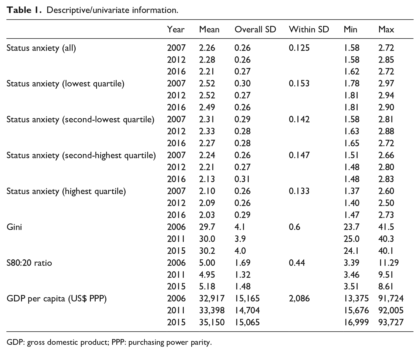
GDP: gross domestic product; PPP: purchasing power parity.

Results

From Table 1, we see that status anxiety (at the level of country averages) overall ranges from approximately 1.6 to 2.8. It is highest in the lowest-earning quartile (range: 1.8–2.95) and lowest in the highest-earning quartile (range: 1.4–2.6). Status anxiety overall increases slightly from 2007 to 2012 and then decreases in 2016; that pattern is evident especially in the second-lowest quartile. Average inequality, as measured via Gini coefficients, increases slightly across this time period for this group of countries, from 29.7 to 30.2. Inspecting the data on individual countries (via the supplementary table in the online supplement), we see divergent trends and, in many instances, larger changes. Inequality increased by more than one (Gini) point in Bulgaria, Denmark, Spain, France, Croatia, Latvia, Luxembourg, Sweden, and Slovenia. Inequality decreased by at least one point in Ireland, Poland, Slovakia, and Turkey. In most instances, a change of (at least) this magnitude happened for these countries already between 2006 and 2011—in line with research showing that the financial crisis of 2008 had divergent effects on inequality (Nolan and Valenzuela, 2019). For the most part, the direction of change is the same when we consider the S80:20 ratio. There are, however, a few discrepancies: for Estonia and Malta in this period, inequality measured by Gini increased while inequality measured by the S80:20 ratio decreased. The opposite pattern is apparent in Hungary. What we see overall, then, is substantial diversity in trends—a feature that makes these data useful for exploring the impact of changes in inequality.

The main results are presented in Table 2. (This table excludes people who did not provide data on their incomes; further consideration of this angle, using imputation for income, is found below.) In general, when inequality increases there is a decrease in status anxiety (Model 1, where b = −0.018). When we consider the impact separately for the different income quartiles, however, we see that this effect varies by position in the income distribution. For people in the lowest quartile, the apparent consequence of increasing inequality is an increase in average levels of status anxiety. For an increase in Gini of one point, average levels of status anxiety increase by 0.034 points (from Model 2).

Table 2.

“Within” models of status anxiety.

	All	Lowest quartile	Second-lowest quartile	Second-highest quartile	Highest quartile
	Model 1	Model 2	Model 3	Model 4	Model 5
Inequality (Gini)	−0.018	0.034	−0.030	−0.058	−0.050
p/c GDP (log)	0.112	−0.220	0.197	0.631	0.786
2012	−0.040	−0.059	−0.085	−0.113	−0.075
2016	0.004	0.006	0.003	−0.098	−0.067
N	87	87	87	87	87
Standardized coefficient for inequality (effect size)	−0.09	0.13	−0.13	−0.24	−0.23

GDP: gross domestic product.

What should we make of this number? In line with the discussion above, I do not propose to divide it by its standard error to decide whether it is “significant.” Instead, we can consider effect size, by using standardized coefficients. For example, for the lowest quartile, we first multiply the coefficient 0.034 × 0.6 (the within standard deviation for the Gini measure) and then divide by 0.157 (the within standard deviation for status anxiety in the lowest quartile). A row at the bottom of Table 2 gives the results in these terms. The effect size for the lowest quartile, then, is −0.13. Using the thresholds associated with Cohen’s d, we see an effect that falls below the threshold of a “small” effect (|0.2|). The apparent increase in status anxiety for this group, following from a typical amount of change in inequality for this group of countries, does not reach the level of a small effect.

For people in the upper two quartiles, on the other hand, increased inequality leads to lower levels of status anxiety, on average. For those in the highest-earning quartile, an increase in one Gini point leads to a decrease in average (country-level) status anxiety of 0.050 points (Model 5). The standardized coefficient for this quartile is −0.23—higher than the threshold for a small effect. For the second-highest quartile, increased inequality also brings reduced status anxiety, and the effect size is almost identical, at −0.24—again representing a decrease in average status anxiety from a typical increase in inequality (as given by the within standard deviation for that variable). For the second-lowest quartile, the effect is negative (a decrease in status anxiety), but the effect size is −0.13—identical to the value for the lowest quartile.

Table 3 presents an equivalent analysis using the S80:20 ratio as a measure of inequality. We now see even more substantial evidence that an increase in inequality brings a reduction in status anxiety for higher earners: the effect size for the top quartile is −0.40, and for the second-highest quartile almost identical at −0.41. For the second-lowest quartile, there is also a reduction in status anxiety (following an increase in inequality), with an effect size of −0.32. For the lowest quartile, the effect is negative as well, but as with the analysis using Gini coefficients, the effect size falls below the threshold for a “small” effect.

Table 3.

“Within” models of status anxiety.

	All	Lowest quartile	Second-lowest quartile	Second-highest quartile	Highest quartile
	Model 1	Model 2	Model 3	Model 4	Model 5
Inequality (S80:20 ratio)	−0.086	−0.045	−0.102	−0.137	−0.121
p/c GDP (log)	−0.127	−0.554	−0.077	0.394	0.597
2012	−0.039	−0.044	−0.088	−0.122	−0.082
2016	0.020	0.042	0.017	−0.092	−0.061
N	85	85	85	85	85
Standardized coefficient for inequality (effect size)	−0.30	−0.13	−0.32	−0.41	−0.40

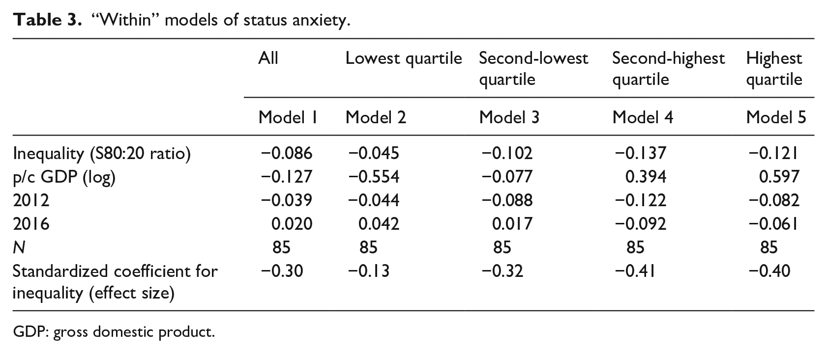
GDP: gross domestic product.

A key question posed in this article is whether inequality is bad for people at the top. The results presented here indicate that the answer to that question is: no. When inequality increases, status anxiety for higher earners goes down; that pattern is apparent not only for people in the highest quartile but also for people in the second-highest quartile. This conclusion is not in line with the idea that higher earners suffer from higher levels of inequality. The only people who might suffer from increased inequality are those in the lowest quartile (though again the effect does not reach the threshold of “small,” and in the analysis using the S80:20 ratio, the coefficient is negative, suggesting lower status anxiety). The effect is indeed different for people in different places on the earnings distribution. A different effect was not discerned in previous research on this topic (e.g. Layte and Whelan, 2014)—in part because the results were interpreted with reference to statistical significance. But statistical significance is not a relevant consideration in this context, because we are not attempting to generalize from a sample of countries to a population of countries.

Increases in inequality appear to enhance the subjective experience of higher earners. This finding is again not consistent with core arguments in the SL: in particular, it undermines the notion that inequality is bad for the vast majority. The survey question used here asks respondents whether people “look down on” them because of their job situation or income, or fail to value what they do. In a conventional perspective on status and subjective well-being, the people at the top can do the “looking down on” those with a lower position—a view that brings psychological benefits (e.g. Clark et al., 2008; see also Morgan, 2019 on “snobbery”). An increase in inequality does not evidently undermine these psychological benefits for higher earners; on the contrary, it enhances them. When inequality increases, people in the middle quartiles (especially the second-highest) also experience enhanced psychological benefits in this sense—results that also undermine the notion that inequality is bad for the vast majority. This result is arguably in line with the idea that some people who are not at the top experience inequality in a “tunnel” mode (Hirschman, 1973), where inequality offers information about gains that might be achieved in the future.

As noted above, the quartile-specific results presented in Tables 2 and 3 use data on status anxiety from respondents who provided information on their household incomes—something a substantial proportion of respondents did not do. Table 4 offers results from an analysis where imputation has been used (in particular for income), to include nonresponders in the calculation of quartile-specific summaries of status anxiety. These results do not lead to consequential changes in the substantive conclusions presented above (a pattern evident also in the work of Layte and Whelan, 2014; Steckermeier and Delhey, 2019). Using Gini coefficients, the effect size for people in the highest quartile is now −0.22 (as against −0.23 when imputation is not used); using the S80:20 inequality measure, the effect size is now −0.36 (as against −0.40). For people in the second-highest quartile, we see a slightly decreased effect size when using the S80:20 inequality measure (−0.31, as against −0.41 without imputation). For people in the lower two quartiles as well, conclusions do not change when the analysis is done with data bolstered by imputation. Addressing nonresponse on income does not lead us to a different conclusion, especially for the core question posed here: we still see that increased inequality has beneficial consequences for higher earners.

Table 4.

“Within” models of status anxiety, using imputed data.

	Using Gini measures				Using S80:20
	Lowest quartile	Second-lowest quartile	Second-highest quartile	Highest quartile	Lowest quartile	Second-lowest quartile	Second-highest quartile	Highest quartile
Inequality	0.037	−0.021	−0.033	−0.049	−0.017	−0.078	−0.105	−0.108
p/c GDP (log)	−0.279	0.016	0.367	0.319	−0.485	−0.209	0.145	0.149
2012	0.042	−0.031	−0.024	0.014	0.059	−0.033	−0.025	0.006
2016	0.028	0.028	−0.046	−0.020	0.058	0.025	−0.032	−0.017
N	87	87	87	87	85	85	85	85
Effect size (inequality)	0.15	−0.09	−0.13	−0.22	−0.05	−0.24	−0.31	−0.36

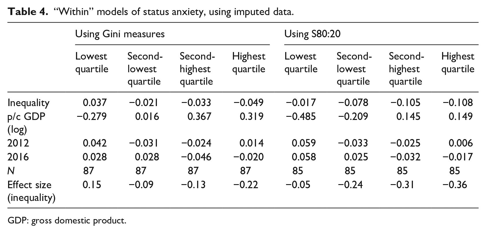
GDP: gross domestic product.

An additional angle that merits attention is the length of the lag from macroeconomic change to subjective outcomes. The analysis above uses a 1-year lag. Plausibly, it might take longer for changes in inequality to affect people’s subjective experiences. To explore that idea, I re-ran the analysis using lags of 2 and 3 years. The substantive conclusions from these models (available on request) are not different from those using the results presented above: we continue to see that increases in inequality lead to reduced status anxiety for people in the top half (the top two quartiles) of the income distribution, while for people at the bottom there is no notable effect.

Conclusion

It might have been satisfying to learn that higher earners suffer from inequality—but that is not what the analysis above tells us. A longitudinal analysis indicates that higher earners experience lower levels of status anxiety, on average, as inequality increases. This finding would have weakened our confidence in the idea that wealthier people could be persuaded to embrace egalitarianism on the basis that they will benefit from it. Any attempt to mitigate inequality for the benefit of lower earners will have to confront the likelihood that higher earners will strive to maintain their advantages. There is a conflict of interests here that cannot be wished away. The “income inequality hypothesis” (IIH) pertaining to health is of course an idea with a long scholarly history (Rodgers, 1979). In more recent years, there is increasing focus on the psychological consequences of inequality, and many studies do find that inequality imposes psychological costs on people who have lower positions in a society (e.g. Buttrick and Oishi, 2017, Sommet et al., 2018). The idea that inequality has negative consequences also for people in higher positions is not altogether implausible—but it is not apparent that there is a sound empirical basis for it in a longitudinal analysis, at least in connection to status anxiety.

The main limitation to mention regarding this conclusion is that the data used here enable an analysis covering a time span (9 years) that is reasonably described as short. Still, a short time span is preferable to no time span at all (as in a cross-sectional analysis). Insofar as the research question posed here is articulated in dialogue with the SL, we can note the different time periods used for empirical analysis: the analysis here uses data from a later time period, relative to the analysis informing Wilkinson and Pickett’s earlier work. On the other hand, the fact that inequality patterns were different in the later time period does not obviously mean that the relationship between inequality and subjective experience would have changed over time. (The time period of the analysis here is more aligned with the empirical work informing The Inner Level.) Another point to bear in mind is that the results here pertain only to European countries.

A third limitation pertains to socioeconomic mobility. The analysis here has used the EQLS income-quartiles variable, at three different points in time, in ways that might seem to assume that the quartiles are populated at each time point by the same sets of individuals. Instead, people’s incomes can of course change, and so the composition of the quartiles can change. That point will perhaps seem less relevant in the context of a cross-sectional analysis, but in a longitudinal framework, there is no escaping it. Unfortunately, in the absence of panel data at the individual level, there is nothing much we can do to address it empirically. We are instead limited to a deductive evaluation, asking about the potential consequences of mobility via implication for our results.

The key issue in those terms is whether there are plausible scenarios that would lead us to a different conclusion regarding inequality’s impact on higher earners. What would have to be true about the mobility of people into (and out of) the top quartile, to arrive at a conclusion where increasing inequality was actually harmful (or perhaps merely benign) to higher earners? Consider a scenario in which what matters for the reduction of people’s status anxiety is not so much earning a higher income but rather achieving a higher income (i.e. upward mobility). The negative coefficients in Models 4 and 5 above (for Tables 2 and 3 alike) might then be rooted mainly in the experiences of those who move up, while people at a stable level (of higher income) are perhaps more vulnerable to anxiety, possibly on the basis of worries that they might not be able to sustain their position. If upward mobility is substantial enough, perhaps the rewarding experiences of the upwardly mobile could outweigh negative subjective experiences among those worried about the possibility of downward mobility. However, we can bear in mind that the “within” analysis addresses a dynamic situation pertaining to changes in inequality, not a static one pertaining to a stable level of inequality. To account for the key results in Tables 2 and 3 (in particular, Models 4 and 5), the hypothetical process described here would have to be exacerbated by increases in inequality. On this basis, it does not seem especially likely that the reduction in status anxieties for higher earners is somehow an artifact of differential processes associated with mobility instead. Still, this is a deductive conclusion rather than an empirical one.

The broader utility of the research reported in this article derives from its form. To investigate the consequences of a country-level variable, researchers can look beyond the conventional format of cross-sectional multilevel modeling so that a longitudinal analysis becomes feasible. Kragten and Rözer (2017) show that there is an important difference between cross-sectional and longitudinal results when investigating the impact of inequality on physical health (the original version of the IIH): a longitudinal analysis reveals a negative impact that is not apparent in a cross-sectional analysis (where omitted variable bias is likely a bigger problem). Delhey and Steckermeier (2020) demonstrate the different conclusions emerging from cross-sectional versus longitudinal analysis of the impact of inequality on “social ills” (a key concept for the SL): in a longitudinal analysis, an increase in inequality does not lead to an increase in the number of “social ills,” despite clear evidence of a cross-sectional association. Similar patterns are evident also in Avendano (2012) and Hu et al. (2015).

This possibility (divergence in findings between cross-sectional and longitudinal results) is likely relevant to the investigation of other country-level variables as well. An additional area for exploration pertains to the impact of policies, especially where there is a measure that captures changes in a policy framework over time (e.g. the Migrant Integration Policies Index, MIPEX—see Bartram and Jarochova, 2022). For policy effects as well, it seems very unlikely that individual-level control variables (e.g. sex, age, education, and religiosity) are relevant as confounders. An analysis that links policy measures to aggregated country-level data from repeated cross-sectional surveys offers an alternative to cross-sectional MLM analyses—an approach that is more robust to omitted variable bias and more in line with a causal question that asks what happens as policies change.

Supplemental Material

sj-xlsx-1-cos-10.1177_00207152221094815 – Supplemental material for Does inequality exacerbate status anxiety among higher earners? A longitudinal evaluation

Supplemental material, sj-xlsx-1-cos-10.1177_00207152221094815 for Does inequality exacerbate status anxiety among higher earners? A longitudinal evaluation by David Bartram in International Journal of Comparative Sociology

Footnotes

Appendix 1 Acknowledgements

I am grateful to Jan Delhey for very useful feedback on an earlier version of the paper, and to the editor and the four anonymous reviewers who engaged with the paper in a highly constructive way.

Availability of data

See below

Code availability

The analysis syntax for this paper is available here:

Declaration of conflicting interests

The author(s) declared no potential conflicts of interest with respect to the research, authorship, and/or publication of this article.

Funding

The author(s) received no financial support for the research, authorship, and/or publication of this article.

ORCID iD

David Bartram

Supplemental material

Supplemental material for this article is available online.

Notes

References

Avendano

(2012) Correlation or causation? Income inequality and infant mortality in fixed effects models in the period 1960–2008 in 34 OECD countries. Social Science & Medicine 75(4): 754–760.

Bartram

(2021) Cross-sectional model-building for research on subjective well-being: Gaining clarity on control variables. Social Indicators Research 155: 725–743.

Bartram

Jarochova

(2022) A longitudinal investigation of integration/multiculturalism policies and attitudes towards immigrants in European countries. Journal of Ethnic and Migration Studies 48(1): 153–172.

Bourdieu

(2010) Distinction: A Social Critique of the Judgement of Taste. London: Routledge.

Brüderl

Ludwig

(2015) Fixed-effects panel regression. In: Best

Wolf

(eds) The SAGE Handbook of Regression Analysis and Causal Inference. Los Angeles, CA: SAGE, pp. 327–357.

Buttrick

Oishi

(2017) The psychological consequences of income inequality. Social and Personality Psychology Compass 11(3): e12304.

Cheung

Lucas

(2016) Income inequality is associated with stronger social comparison effects: The effect of relative income on life satisfaction. Journal of Personality and Social Psychology 110(2): 332–341.

Clark

Frijters

Shields

(2008) Relative income, happiness and utility: An explanation for the Easterlin Paradox and other puzzles. Journal of Economic Literature 46(1): 95–144.

Delhey

Steckermeier

(2020) Social ills in rich countries: New evidence on levels, causes, and mediators. Social Indicators Research 149(1): 87–125.

10.

Delhey

Schneickert

Steckermeier

(2017) Sociocultural inequalities and status anxiety: Redirecting the spirit level theory. International Journal of Comparative Sociology 58(3): 215–240.

11.

Dorling

(2019) Inequality and the 1%. London: Verso.

12.

Engman

(2013) Is there life after P<0.05? Statistical significance and quantitative sociology. Quality & Quantity 47(1): 257–270.

13.

European Quality of Life Survey (EQLS) and European Foundation for the Improvement of Living and Working Conditions (2018) EQLS integrated data file, 2003-2016. UK Data Service. Available at: http://doc.ukdataservice.ac.uk/doc/7348/mrdoc/UKDA/UKDA_Study_7348_Information.htm

14.

Frank

(2008) Richistan: A Journey through the 21st Century Wealth Boom and the Lives of the New Rich. London: Piatkus.

15.

Friedman

O’Brien

McDonald

(2021) Deflecting privilege: Class identity and the intergenerational self. Sociology 55(4): 716–733.

16.

Gangl

(2010) Causal inference in sociological research. Annual Review of Sociology 36(1): 21–47.

17.

Hirschman

(1973) The changing tolerance for income inequality in the course of economic development. The Quarterly Journal of Economics 87(4): 544.

18.

van Lenthe

Mackenbach

(2015) Income inequality, life expectancy and cause-specific mortality in 43 European countries, 1987–2008: A fixed effects study. European Journal of Epidemiology 30(8): 615–625.

19.

Kragten

Rözer

(2017) The income inequality hypothesis revisited: Assessing the hypothesis using four methodological approaches. Social Indicators Research 131(3): 1015–1033.

20.

Layte

Whelan

(2014) Who feels inferior? A test of the status anxiety hypothesis of social inequalities in health. European Sociological Review 30(4): 525–535.

21.

Loughnan

Kuppens

Allik

, et al. (2011) Economic inequality is linked to biased self-perception. Psychological Science 22(10): 1254–1258.

22.

Lucas

(2014) An inconvenient dataset: Bias and inappropriate inference with the multilevel model. Quality & Quantity 48(3): 1619–1649.

23.

Marmot

Adelstein

Robinson

, et al. (1978) Changing social-class distribution of heart disease. BMJ 2(6145): 1109–1112.

24.

Marmot

Stansfeld

Patel

, et al. (1991) Health inequalities among British civil servants: The Whitehall II study. The Lancet 337(8754): 1387–1393.

25.

Mills

(2012) Open letter to Prof. Richard Wilkinson & Prof. Kate Pickett. Oxford Sociology Blog. Available at: http://oxfordsociology.blogspot.com/2012/11/open-letter-to-prof-richard-wilkinson.html

26.

Morgan

(2019) Snobbery. London: Policy Press.

27.

Morgan

Winship

(2007) Counterfactuals and Causal Inference: Methods and Principles for Social Research. Cambridge: Cambridge University Press.

28.

Niskanen

Moore

(1996) Supply-side tax cuts and the truth about the Reagan economic record. Cato Institute Policy Analysis No. 261. Available at: https://www.cato.org/sites/cato.org/files/pubs/pdf/pa261.pdf

29.

Nolan

Valenzuela

(2019) Inequality and its discontents. Oxford Review of Economic Policy 35(3): 396–430.

30.

Offer

(2006) The Challenge of Affluence: Self-Control and Well-Being in the United States and Britain since 1950. Oxford: Oxford University Press.

31.

Paskov

Gërxhani

Werfhorst

(2017) Giving up on the Joneses? The relationship between income inequality and status-seeking. European Sociological Review 33(1): 112–123.

32.

Pearl

Mackenzie

(2018) The Book of Why: The New Science of Cause and Effect. London: Allen Lane.

33.

Ridgeway

(2014) Why status matters for inequality. American Sociological Review 79(1): 1–16.

34.

Robinson

(1950) Ecological correlations and the behavior of individuals. American Sociological Review 15(3): 351–357.

35.

Rodgers

(1979) Income and inequality as determinants of mortality: An international cross-section analysis. Population Studies 33(2): 343–351.

36.

Rubin

(1987) Multiple Imputation for Nonresponse in Surveys. New York: John Wiley.

37.

Schneider

(2019) Why income inequality is dissatisfying—Perceptions of social status and the inequality-satisfaction link in Europe. European Sociological Review 35(3): 409–430.

38.

Solt

(2019) The standardized world income inequality database, versions 8-9. Harvard Dataverse. Available at: https://dataverse.harvard.edu/dataset.xhtml?persistentId=doi:10.7910/DVN/LM4OWF

39.

Solt

(2020) Measuring income inequality across countries and over time: The standardized world income inequality database. Social Science Quarterly 101(3): 1183–1199.

40.

Sommet

Morselli

Spini

(2018) Income inequality affects the psychological health of only the people facing scarcity. Psychological Science 29(12): 1911–1921.

41.

Steckermeier

Delhey

(2019) Better for everyone? Egalitarian culture and social wellbeing in Europe. Social Indicators Research 143(3): 1075–1108.

42.

Van de Werfhorst

Salverda

(2012) Consequences of economic inequality: Introduction to a special issue. Research in Social Stratification and Mobility 30(4): 377–387.

43.

Veblen

(1994 [1899]) The Theory of the Leisure Class. New York: Penguin Books.

44.

Walasek

Brown

GDA

(2016) Income inequality, income, and internet searches for status goods: A cross-national study of the association between inequality and well-being. Social Indicators Research 129(3): 1001–1014.

45.

Wilkinson

Pickett

(2010) The Spirit Level: Why Greater Equality Makes Societies Stronger. New York: Bloomsbury Press.

46.

Wilkinson

Pickett

(2019) The Inner Level: How More Equal Societies Reduce Stress, Restore Sanity and Improve Everyone’s Well-Being. London: Allen Lane.

Supplementary Material

Please find the following supplemental material available below.

For Open Access articles published under a Creative Commons License, all supplemental material carries the same license as the article it is associated with.

For non-Open Access articles published, all supplemental material carries a non-exclusive license, and permission requests for re-use of supplemental material or any part of supplemental material shall be sent directly to the copyright owner as specified in the copyright notice associated with the article.

0.00 MB

0.01 MB