Active tracking and decoupling control of pavement temperature for icing early-warning

Abstract

Pavement icing induced by complex temperature fluctuations during winter weather poses a significant safety hazard. Given that existing icing detection methods are predominantly passive, this study designs an active pavement temperature simulation device based on a thermoelectric cooler (TEC). Using the predicted pavement temperature as the thermal control target, the device achieves dynamic temperature tracking and simulates both the pavement temperature and ice-snow status through active cooling. A temperature control model for the device is established by incorporating heat transfer theory and applying small-signal analysis methods. To address the system’s inherent nonlinear and coupled characteristics, a fuzzy adaptive PID decoupling control strategy is proposed. This strategy enables accurate pavement temperature tracking and facilitates active early warnings for runway icing. The results demonstrate that under typical input signals, the proposed control method exhibits excellent steady-state performance, high tracking accuracy, and robust anti-interference capability. Specifically, the active simulation device tracks the target temperature with a steady-state error not exceeding 0.08°C. The tracking error follows a normal distribution, with 99.7% of the error samples falling within ± 0.2°C. This performance improvement is statistically significant compared to traditional PID control (p < 0.05), thereby effectively simulating the thermal evolution of the runway surface. Ultimately, this research provides a novel approach for active runway icing early warnings, aligning with the Global Reporting Format (GRF).

Keywords

pavement temperature active icing early warning thermoelectric cooling decoupling control temperature tracking

Introduction

Runway icing significantly reduces the friction between aircraft wheels and the pavement surface, severely compromising flight operational safety and posing a critical threat to civil aviation operations. The GRF issued by the International Civil Aviation Organization (ICAO) establishes standardized requirements for the assessment and reporting of runway surface conditions, emphasizing the need for systematic evaluation based on multiple parameters, such as pavement state and friction coefficient, to achieve more accurate and consistent runway condition assessments. The GRF standard not only requires accurate feedback on current runway surface conditions but also outlines clear technical requirements for the forward-looking prediction of runway icing risk and the consistency of condition assessments across different airports. Within this framework, obtaining timely information on the runway icing status and effectively predicting temperature changes have become critical for ensuring the safe operation of runways. Many airports still face challenges in managing runway icing, such as delayed responses to temperature variations, passive judgment of icing conditions, and untimely information feedback. Because they currently rely on passive identification after icing occurs, these airports cannot provide effective data support for the proactive risk early warning and standardized condition reporting required by the GRF standard, making it difficult to fully meet the real-time and accuracy requirements stipulated by the GRF. Pavement temperature is a key variable affecting ice formation, and its accurate short-term prediction will contribute to identifying critical temperature thresholds for runway icing, thereby providing essential information for GRF-compliant runway condition assessments and active icing early warnings.

Research on pavement temperature prediction is primarily categorized into theoretical and statistical methodologies. The theoretical approach, grounded in heat transfer theory, establishes predictive models by numerically solving heat conduction differential equations governing the surface temperature field.¹ Conversely, the statistical methodology primarily employs machine learning techniques, utilizing extensive historical temperature measurements and meteorological data as training samples to derive the mapping relationships between various factors and temperature, thereby constructing predictive models. Nuijten and Høyland established a comprehensive thermal conduction equation for airport runways, employing the finite difference method to determine the temperature field within the runway structure at various depths.^2,3 Klein-Paste et al. proposed the IRIS runway model to accurately predict the surface conditions of contaminated runways under winter weather, demonstrating the model’s high accuracy and adaptability.⁴ Hermansson developed a pavement temperature field model accounting for the effects of solar radiation, air temperature, and wind speed, validating it through a comparative analysis with measured data.^5,6 Sun and Qin utilized regression fitting methods based on field-measured data to estimate the temperature field of asphalt pavements.^7,8 Yavuzturk et al. employed a two-dimensional finite difference model to calculate the transient temperature field distribution, accurately predicting temperature variations at different pavement locations.⁹ Dave and Buttlar investigated thermal reflective cracking using finite element pavement models and structural parameters, verifying the model’s accuracy through case studies.¹⁰ Chen et al. introduced a three-dimensional transient temperature field analysis method to simplify the complex heat exchange system of pavements, deriving a pavement temperature function through the regression analysis of measured data.¹¹ However, this review indicates that the statistical approach’s heavy reliance on extensive meteorological data inherently limits its applicability across diverse geographical regions and fails to account for the dynamic thermal properties of runway materials under current operational conditions. To address these limitations, this paper proposes a theoretical analysis method that incorporates comprehensive boundary condition constraints into the model. This enhancement enables the pavement temperature prediction model to accurately characterize the evolutionary patterns of temperature variations across various environmental and operational scenarios.

Significant research has been conducted on runway icing prediction and detection.^12–14 Analyzing the differences in the physical properties of ice and water enables the precise identification of runway icing conditions. However, these technologies are primarily categorized as passive icing detection, which possesses inherent limitations. In contrast, active icing detection methods remain relatively scarce. Therefore, this study proposes employing TECs as the core temperature control devices. TECs feature a straightforward structure, high temperature control precision, and exceptionally low thermal inertia. This approach facilitates active temperature reduction, thereby establishing a proactive runway icing early warning system. While numerous studies have explored the temperature control of TECs, most current systems are applied to constant temperature control scenarios, such as semiconductor lasers and precision instruments. Their control objectives are mostly fixed temperature setpoints, with a primary focus on improving steady-state temperature control accuracy. They fail to account for the dynamic, time-varying target tracking requirements of the controlled object, nor do they adapt multi-field coupling models or optimize control strategies specifically for the airport runway icing early warning scenario. Therefore, they cannot be directly applied to the core requirements of continuous dynamic tracking of runway pavement temperature and icing state simulation. Extensive research on TEC temperature control strategies has proposed various methodologies. Early control strategies were largely based on PID control.¹⁵ PID control achieves its objective by monitoring the error between actual and target values and adjusting the system output in real time. However, due to the inherent nonlinear characteristics of TECs, traditional PID control often fails to meet performance requirements. Zhai and Chai developed a precise temperature control system for semiconductor lasers by integrating genetic algorithms (GAs) with PID control.¹⁶ However, the encoding and decoding processes inherent to GAs are computationally intensive, which increases overall system complexity. To address the significant nonlinearity and susceptibility to strong disturbances of the controlled object, Song et al. established a linear dynamic model for TECs using small-signal linearization techniques and proposed a fuzzy adaptive PID control strategy.¹⁷ Numerical analysis and experimental results demonstrate that this system achieves excellent steady-state performance and exhibits robust disturbance rejection. These findings underscore the critical importance of accounting for nonlinear characteristics to achieve effective temperature control in TECs. Thus, developing tailored temperature control strategies is essential to meet the complex requirements of TEC applications.

Active icing detection is distinct from traditional passive icing detection, which only identifies the icing status after ice has formed. At its core, this approach utilizes a built-in active excitation unit that continuously emits specific forms of energy—such as optical, electrical, acoustic, or mechanical vibration—to the measured area, collects feedback signals in real time, and achieves full-cycle monitoring through changes in medium characteristics. It not only identifies the icing status but also quantitatively measures ice thickness, differentiates between ice types and phase states, tracks the entire icing process, and acquires key information, including critical icing parameters (freezing point, icing rate), pavement covering type, and icing risk level. It represents a crucial cutting-edge technology for icing prevention and control in applications such as airport runways, expressways, aerospace, and wind turbine blades. Ikiades designed a fiber-optic icing sensor. By analyzing the optical and diffusion characteristics of light in different types of ice, this sensor enabled the measurement of ice thickness and identification of icing type after calibration.¹⁸ Experimental results demonstrated that the sensor can measure ice layers up to 10 mm thick with a measurement accuracy of approximately 0.5 mm. Wang et al. and Gui et al. designed a resonant icing sensor based on piezoelectric devices. When water accumulates or ice forms on the sensor surface, the equivalent mass and stiffness of the entire sensing system change, which in turn causes a shift in the resonant frequency output by the sensor, enabling the accurate identification of three pavement conditions: dry, water-covered, and iced.^19,20 A research team from Taiyuan University of Technology designed multiple pairs of parallel capacitive plates connected in parallel for detecting the icing thickness of rivers in winter.²¹ The icing thickness is calculated by measuring the output capacitance value, counting the number of plates with ice as the filling medium, and incorporating the height of the plates. In contrast to the above three types of sensing schemes, TEC active icing monitoring technology is developed based on the underlying thermophysical properties of the medium. It is immune to interference from external factors such as optical contamination, mechanical vibration, and dielectric constant drift, and exhibits exceptional adaptability to extreme environments. This effectively addresses the core limitations of traditional schemes: the difficulty in critical phase state identification and insufficient quantitative measurement accuracy.

This study establishes a mechanistic model based on heat transfer principles for predicting pavement temperature under freezing weather conditions. The predicted temperature serves as the control target for an active simulation device. Compared with existing TEC temperature control systems, the key innovations of this study are as follows: First, overcoming the inherent “fixed-target constant temperature control” mode of traditional systems, this study establishes an active temperature control framework that utilizes the dynamic predicted value of pavement temperature as the real-time tracking target, thereby achieving continuous dynamic tracking of the pavement temperature evolution process. Second, to address the strong coupling and nonlinear characteristics between the cold and hot ends of the TEC, a fuzzy adaptive PID decoupling control strategy is proposed. This approach resolves critical industry challenges regarding response lag and insufficient disturbance rejection capabilities in TEC systems under dynamic target tracking. Third, TEC active temperature control technology is deeply integrated with the critical state identification of runway icing for the first time, realizing a technological leap from “the passive detection of existing ice” to “the active simulation and prediction of the icing formation process.” Specifically, a linear dynamic model of this device is developed using heat transfer theory combined with small-signal analysis. To address the coupling between the device’s cold and hot ends, a decoupling method is employed, transforming the multiple-input multiple-output (MIMO) system into a single-input single-output (SISO) system, thereby enhancing temperature control precision. Considering potential variations in the device model under practical operating conditions, the proposed fuzzy adaptive PID control strategy provides further improvement. Precise temperature control of the device enables accurate tracking of pavement temperature and the active simulation of ice and snow conditions, which provides a novel technical solution for the implementation and application of GRF standards under winter weather conditions.

Pavement temperature prediction

Pavement surface heat flux balance equation

As illustrated in Figure 1, the asphalt pavement structure experiences three distinct modes of energy exchange under snowy and icy conditions: radiative heat transfer q_rad, convective heat transfer q_conv, and conductive heat transfer q_cond.²² When atmospheric airflow passes over the runway surface, convective heat transfer occurs due to the temperature difference between the airflow and the pavement, manifesting as sensible heat and latent heat fluxes HE and LE. Solar radiation penetrating the atmosphere reaches the runway, where a portion is directly absorbed as shortwave solar radiation q_s, while another portion, scattered by the atmosphere, contributes to downward atmospheric longwave radiation q_L. Simultaneously, the runway surface emits energy back to the atmosphere via upward longwave radiation q_d. During precipitation events (rain or snow), heat fluxes (q_rain, q_snow) are generated by the temperature differences between the runway and the water film or accumulated snow layer on its surface, with q_melt representing the heat flux associated with snow melting. Additionally, aircraft operations during takeoff and landing generate a distinct heat flux R.

Figure 1.

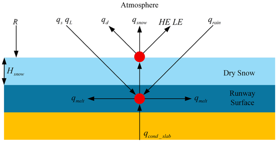
Schematic diagram of surface heat exchange under ice and snow weather.

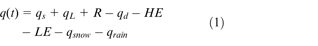
Therefore, considering the heat fluxes from all influencing factors around the runway, the thermal equilibrium equation is derived based on the law of energy conservation:

\begin{matrix} q (t) = q_{s} + q_{L} + R - q_{d} - HE \\ - LE - q_{snow} - q_{rain} \end{matrix}

(1)

Mechanism model for pavement temperature prediction under icy weather conditions

To establish a mechanistic model for pavement temperature prediction, it is essential to solve the temperature field model of the runway subject to complex boundary conditions. Assuming that the temperature at any point within the pavement temperature field is independent of its horizontal position and solely dependent on the depth, the one-dimensional pavement temperature field model can be expressed as ²³:

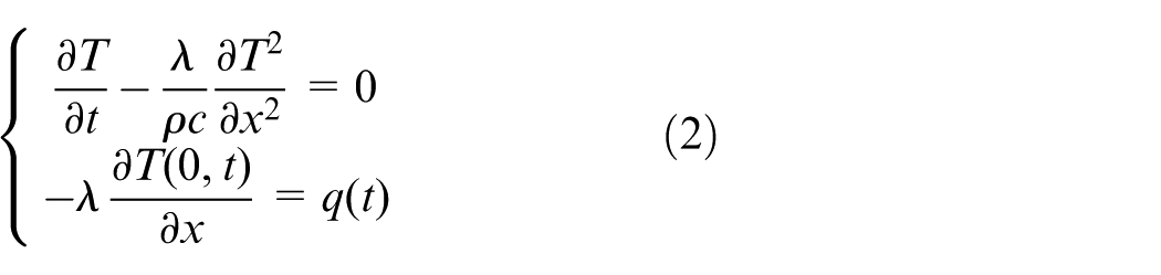
{\begin{matrix} \frac{\partial T}{\partial t} - \frac{λ}{ρ c} \frac{\partial T^{2}}{\partial x^{2}} = 0 \\ - λ \frac{\partial T (0, t)}{\partial x} = q (t) \end{matrix}

(2)

In equation (2), T is the pavement temperature in Kelvin (K); λ is the thermal conductivity coefficient of the runway material in W/(m·K); ρ is the density of the runway material in kg/m³; c is the specific heat capacity of the runway material in J/(kg·K); x is the coordinate along the depth direction of the runway; T(0,t) is the pavement surface temperature at time t; and q(t) is the total heat flux due to heat exchange between the runway and its surrounding environment at time t.

By integrating equations (1) and (2) and applying the finite difference method, the derivatives are approximated using differential quotients, establishing the mechanistic pavement temperature prediction model as follows:

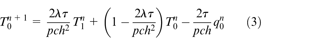
T_{0}^{n + 1} = \frac{2 λ τ}{{pch}^{2}} T_{1}^{n} + (1 - \frac{2 λ τ}{{pch}^{2}}) T_{0}^{n} - \frac{2 τ}{pch} q_{0}^{n}

(3)

In equation (3), $T_{0}^{n}$ represents the pavement surface temperature at the current time instant, $T_{1}^{n}$ denotes the temperature at depth h at the current time instant, $q_{0}^{n}$ signifies the total heat flux at the pavement surface at the current time instant, and $T_{0}^{n + 1}$ indicates the pavement surface temperature after time interval $τ$ .

Dynamic modeling of active pavement temperature simulation system

Active simulation device architecture

The schematic of the proposed buried active simulation device is shown in Figure 2. A TEC is selected as the core refrigeration component, offering a simple structure, high control precision, and low thermal inertia to achieve active cooling.²⁴ Appropriate heat sinks are integrated into both the cold and hot ends. The encapsulated device is buried within the runway, with its cold-end substrate flush with the pavement surface. When powered, the cold-end substrate absorbs surface heat and transfers it via thermal conduction to the hot-end heat sink, thereby enabling active cooling. A temperature sensor embedded in the cold-end heat sink monitors the surface temperature of the cold-end substrate in real time. If this temperature falls below the freezing point of water, ice forms on the device surface. This process enables active ice detection, thereby enhancing early warning capabilities for ice accumulation.

Figure 2.

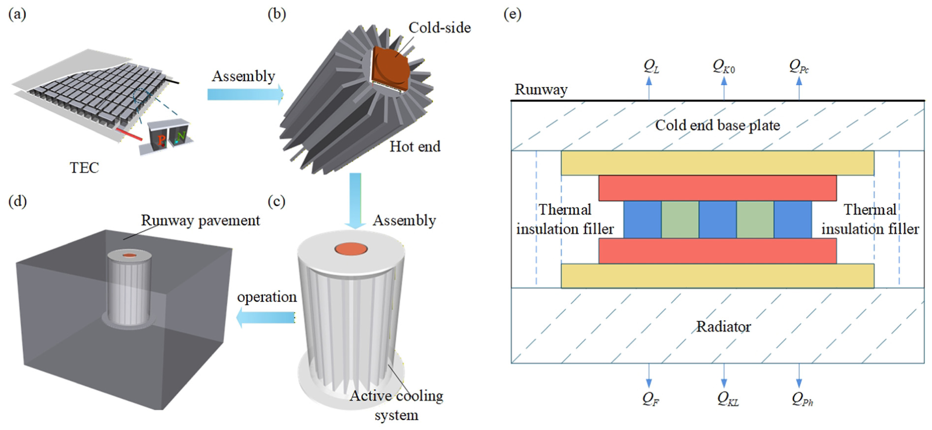
Structural design diagram of active simulation device: (a) TEC model, (b) main assembly, (c) device model, (d) actual environment model and (e) cross-sectional view of the device.

Dynamic modeling of active simulation devices

Control equations

According to the equation of conservation of energy, it can be concluded that:

(C_{L} M_{L} + C_{C} M_{C}) \frac{{dT}_{c}}{dt} = Q_{L} - Q_{K 0} - I α_{m} T_{c}

(4)

In equation (4), M_L and C_L denote the mass and specific heat capacity of the cold-side load, respectively; M_C and C_C represent the mass and specific heat capacity of the cold-side substrate; Q_L indicates the total heat load on the device surface; Q_K0 denotes the conductive heat loss at the TEC cold-side contact surface; I is the operating current through the TEC; a_m is the Seebeck coefficient; and T_C represents the cold-side temperature.

The energy balance of thermoelectric materials yields:

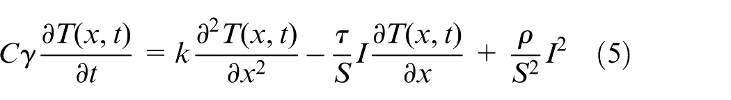
C γ \frac{\partial T (x, t)}{\partial t} = k \frac{\partial^{2} T (x, t)}{\partial x^{2}} - \frac{τ}{S} I \frac{\partial T (x, t)}{\partial x} + \frac{ρ}{S^{2}} I^{2}

(5)

In equation (5), C represents the average specific heat capacity of the thermoelectric material; y denotes the density of the thermoelectric material; K signifies the thermal conductivity of the TEC; T(x,t) describes the thermal distribution within the thermoelectric cooling module; τ stands for the Thomson coefficient; s corresponds to the total surface area of the thermoelectric cooling material; and ρ represents the average resistivity of the thermoelectric material.

The energy conservation equation for the hot-end load of the active simulation device is expressed as follows:

(C_{H} M_{H} + C_{F} M_{F}) \frac{{dT}_{h}}{dt} = α_{m} {IT}_{h} + Q_{KL} - Q_{F}

(6)

In equation (6), M_H and C_H represent the mass and specific heat capacity of the hot-side substrate, respectively; M_F and C_F represent the mass and specific heat capacity of the heat sink; T_h is the hot-side temperature; Q_KL represents the conductive heat dissipation at the TEC hot-side contact surface; and Q_F indicates the conductive, convective, and radiative heat losses from the heat sink.

Model linearization

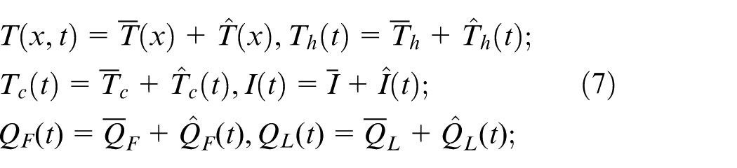
As outlined in Section 3.2.1, the dynamic model of the active simulation device is inherently nonlinear. Since the control methodology relies on linear system and control theory for controller design, the small-signal analysis approach is employed to linearize the system. Specifically, all variables in equations (4)–(6) are expressed as the sum of their steady-state values and perturbation components.

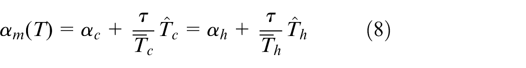
\begin{matrix} T (x, t) = \bar{T} (x) + \hat{T} (x), T_{h} (t) = {\bar{T}}_{h} + {\hat{T}}_{h} (t); \\ T_{c} (t) = {\bar{T}}_{c} + {\hat{T}}_{c} (t), I (t) = \bar{I} + \hat{I} (t); \\ Q_{F} (t) = {\bar{Q}}_{F} + {\hat{Q}}_{F} (t), Q_{L} (t) = {\bar{Q}}_{L} + {\hat{Q}}_{L} (t); \end{matrix}

(7)

The approximate expression for the Seebeck coefficient obtained from Taylor series expansion is ²⁵:

α_{m} (T) = α_{c} + \frac{τ}{{\bar{T}}_{c}} {\hat{T}}_{c} = α_{h} + \frac{τ}{{\bar{T}}_{h}} {\hat{T}}_{h}

(8)

Substituting equations (7) and (8) into equations (4)–(6) yields:

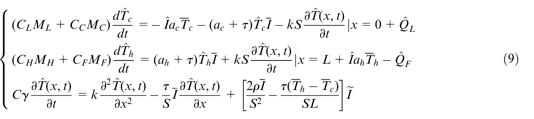
{\begin{matrix} (C_{L} M_{L} + C_{C} M_{C}) \frac{d {\hat{T}}_{c}}{dt} = - \hat{I} a_{c} {\bar{T}}_{c} - (a_{c} + τ) {\hat{T}}_{c} \bar{I} - kS \frac{\partial \hat{T} (x, t)}{\partial t} | x = 0 + {\hat{Q}}_{L} \\ (C_{H} M_{H} + C_{F} M_{F}) \frac{d {\hat{T}}_{h}}{dt} = (a_{h} + τ) {\hat{T}}_{h} \bar{I} + kS \frac{\partial \hat{T} (x, t)}{\partial t} | x = L + \hat{I} a_{h} {\bar{T}}_{h} - {\hat{Q}}_{F} \\ C γ \frac{\partial \hat{T} (x, t)}{\partial t} = k \frac{\partial^{2} \hat{T} (x, t)}{\partial x^{2}} - \frac{τ}{S} \bar{I} \frac{\partial \hat{T} (x, t)}{\partial x} + [\frac{2 ρ \bar{I}}{S^{2}} - \frac{τ ({\bar{T}}_{h} - {\bar{T}}_{c})}{SL}] \tilde{I} \end{matrix}

(9)

Applying the Laplace transform to equation (9) yields:

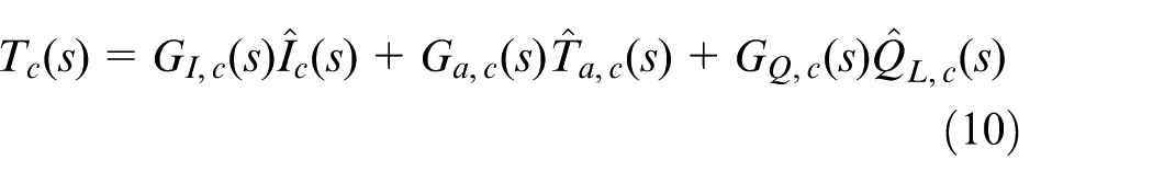
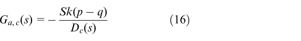
T_{c} (s) = G_{I, c} (s) {\hat{I}}_{c} (s) + G_{a, c} (s) {\hat{T}}_{a, c} (s) + G_{Q, c} (s) {\hat{Q}}_{L, c} (s)

(10)

The detailed definitions and physical meanings of each transfer function in equation (10) are as follows:

Current-to-cold-end temperature transfer function G_I,C(s)

G_{I, c} (s) = \frac{A + B}{sC γ D_{c} (s)}

(11)

\begin{matrix} A = Sk β {(p - q) + [q \cosh (Lp) - p \cosh (Lq)] \\ + [q \sinh (Lp) - p \sinh (Lq)]} \end{matrix}

(12)

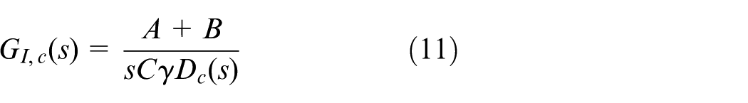
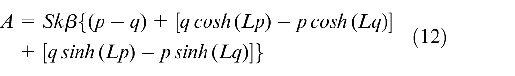
Herein, this term characterizes the coupling effect between the thermal conduction characteristics of the thermoelectric material and the input current, reflecting the heat transfer process that occurs as current passes through the material.

\begin{matrix} B = sC {\bar{T}}_{c} α_{c} γ [\cosh (Lp) - \cosh (Lq) \\ + \sinh (Lp) - \sinh (Lq)] \end{matrix}

(13)

This term reflects the correlation between the steady-state temperature of the cold end and the thermoelectric material’s specific heat capacity and Seebeck coefficient, as well as the influence of this steady-state temperature on the temperature regulation process via current control.

\begin{matrix} D_{c} (s) = E_{c} [\cosh (Lp) - \cosh (Lq) \\ + \sinh (Lp) - \sinh (Lq)] \\ + Sk [p \cosh (Lq) - q \cosh (Lp) \\ + p \sinh (Lq) - q \sinh (Lp)] \end{matrix}

(14)

E_{c} (s) = (M_{L} C_{L} + M_{C} C_{C}) s + (τ + α_{c}) \bar{I}

(15)

D _C(s) serves as the system’s characteristic denominator, consolidating the thermal inertia of the cold-side load and the substrate with the thermal properties of the thermoelectric material to reflect the system’s dynamic response characteristics.

Overall, G_I,S(s) captures the regulatory influence of input current variations on the cold-side temperature, functioning as the core transfer function for current-driven cold-side thermal regulation.

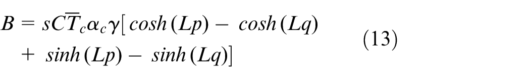
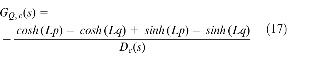
Ambient temperature-to-cold-end temperature transfer function G_a,c(s)

G_{a, c} (s) = - \frac{Sk (p - q)}{D_{c} (s)}

(16)

This transfer function characterizes the effect of ambient temperature fluctuations on the cold-side temperature, where Sk(p-q) reflects the heat conduction intensity between the ambient environment and the cold side. Furthermore, the negative sign indicates an inverse correlation between the variation trends of the ambient temperature and the cold-side temperature.

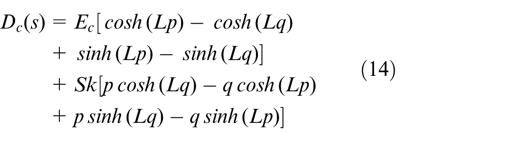
Load-to-cold-end temperature transfer function G_Q,C(s)

\begin{matrix} G_{Q, c} (s) = \\ - \frac{\cosh (Lp) - \cosh (Lq) + \sinh (Lp) - \sinh (Lq)}{D_{c} (s)} \end{matrix}

(17)

This transfer function characterizes the effect of pavement load variations on the cold-side temperature, and reflects the influence characteristics of pavement thermal load fluctuations on the cold-end temperature.

The hot-side temperature of the active simulation device is similarly influenced by the input current, substrate temperature, and hot-side load. The corresponding transfer functions, derived via an analogous procedure, exhibit structural characteristics consistent with those of their cold-side counterparts. To better elucidate the system’s signal transfer dynamics, the corresponding block diagram is depicted as follows (Figure 3):

Figure 3.

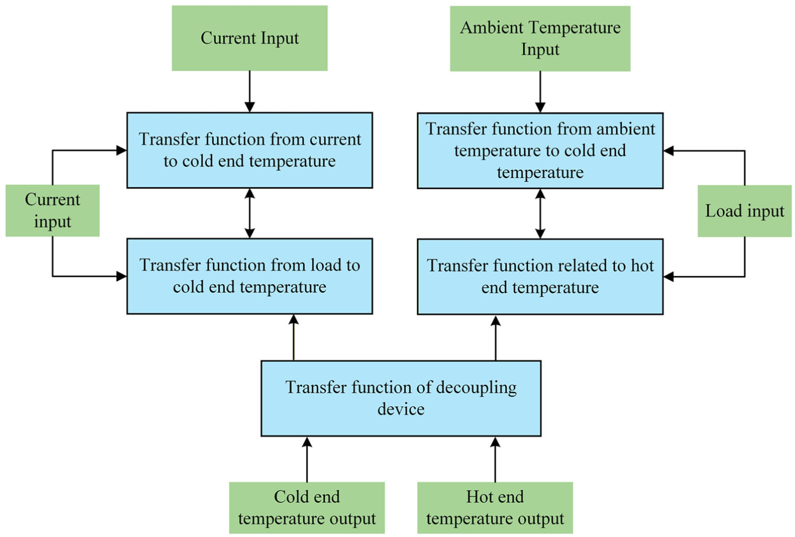
System transfer function block diagram.

This block diagram explicitly delineates the transfer paths from the input current, ambient temperature, and load disturbances to the cold-side and hot-side temperatures, while also highlighting the role of the decoupling device within the system. Furthermore, it visually encapsulates the system’s inherently MIMO characteristics and its comprehensive decoupling control architecture.

Active simulation device tracking method for pavement temperature

Structural diagram of pavement temperature monitoring system

To achieve precise pavement temperature tracking, a dedicated tracking system (Figure 4) has been developed. This system utilizes predicted pavement temperature values derived from a mechanistic prediction model under current weather conditions as the tracking target for the active simulation device. Given that the device model is subject to variations under dynamic operating conditions, an effective temperature control strategy is essential to ensure the accurate tracking of these predicted values (Figure 4).

Figure 4.

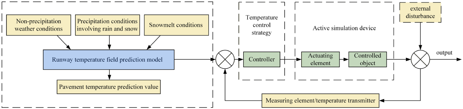
Structural diagram of pavement temperature tracking simulation system.

Control system strategy

Active simulation device temperature control strategy

Analysis of active simulation device characteristics

As detailed in Section 3.2, the active simulation device represents a MIMO system characterized by inherent nonlinearity and thermal coupling. To address the coupling effects between the cold and hot ends of the device, a decoupling control strategy is proposed, transforming the coupled system into a SISO system to further improve temperature control accuracy.²⁶ Unlike the fixed-target steady-state control adopted by existing TEC temperature control systems, the core control requirement of the proposed device is the real-time tracking of dynamic targets, demanding superior response speed, dynamic tracking accuracy, and disturbance rejection performance. Since conventional digital PID controllers struggle to adapt to system parameter variations and exhibit significant hysteresis and time delays, a fuzzy adaptive PID control strategy is implemented to overcome these limitations.²⁷

Design of fuzzy adaptive PID decoupling controller

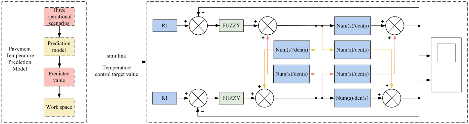
The cold-end and hot-end temperatures are critical control variables in the temperature control system of the active simulation device. The cold-end temperature serves as a key indicator of the device’s cooling performance, while the hot-end temperature significantly influences operational heat dissipation. To meet the control objectives of the active simulation device, this study utilizes ambient and foundation temperatures as inputs. Two PID controllers are then implemented in a cascade configuration to regulate the decoupled subsystems. Furthermore, a fuzzy adaptive PID control strategy is introduced to enhance the device’s temperature control precision. The block diagram of this temperature control system is illustrated in Figure 5.

Figure 5.

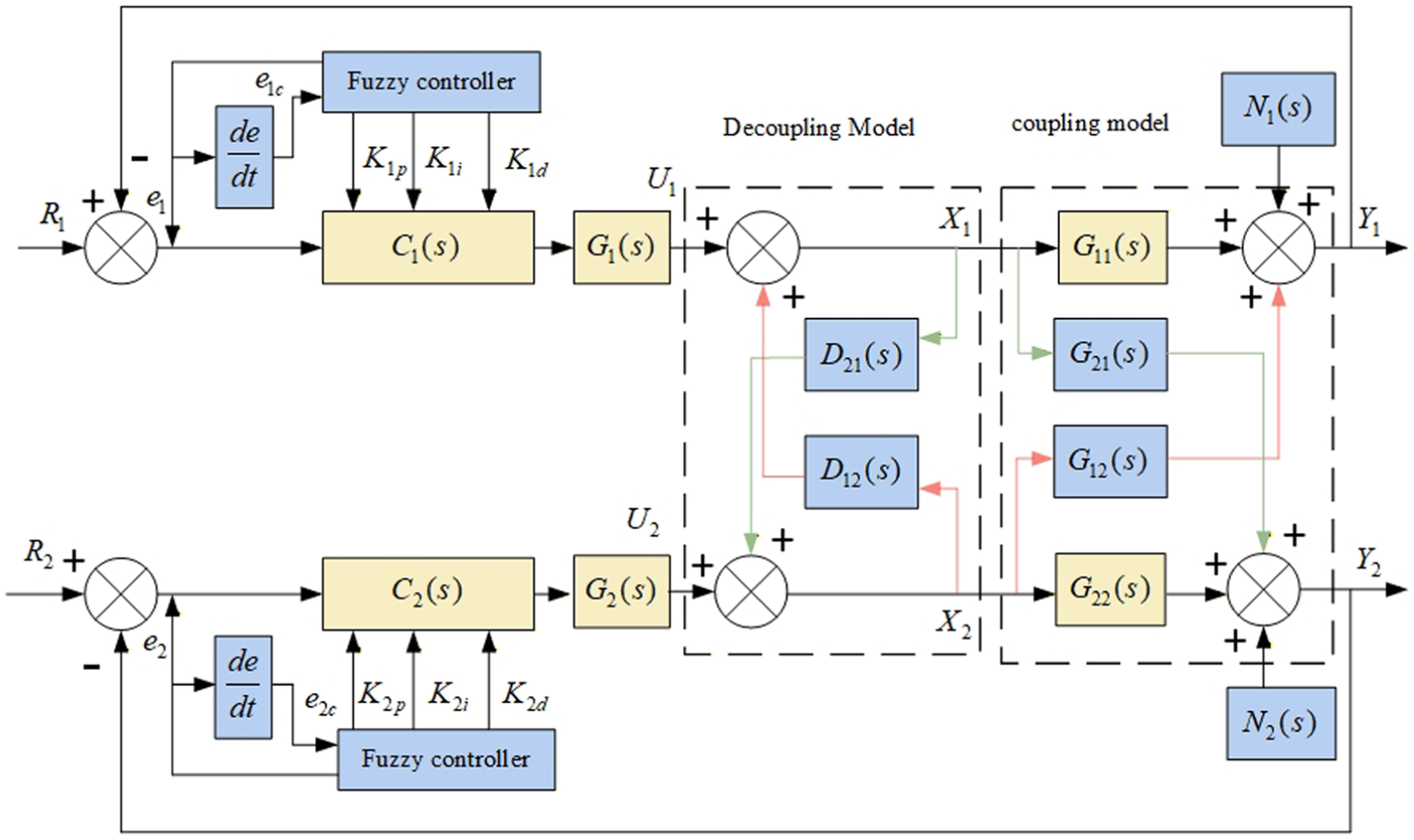
Block diagram of decoupling control based on fuzzy adaptive PID.

In Figure 4, C₁(s) and C₂(s) represent the fuzzy adaptive PID controllers for the cold- and hot-end temperatures, respectively. G₁(s) and G₂(s) are the transfer functions of the cold- and hot-end temperature processes. G₁₁(s), G₂₁(s), G₁₂(s), and G₂₂(s) denote the transfer functions linking the ambient and ground temperatures to the cold- and hot-end temperatures. D₁₂(s) and D₂₁(s) represent the transfer functions of the decouplers. R₁ and R₂ are the setpoints for the cold- and hot-end temperatures, respectively. e₁ and e₂ indicate the corresponding tracking errors (i.e. the deviations between the setpoints and actual values). U₁ and U₂ are the outputs of the respective controllers. Finally, X₁ and X₂ represent the ambient and ground temperature disturbances, while Y₁ and Y₂ are the actual cold- and hot-end temperatures.

Controller parameter tuning methods

The controller parameter tuning process in this study is divided into three stages: decoupling network parameter tuning, basic PID parameter pre-tuning, and fuzzy adaptive online tuning. The entire tuning procedure is conducted on the decoupled SISO system, as detailed below:

Decoupling network parameter tuning

A feedforward compensation diagonal matrix decoupling method is employed to eliminate the cross-coupling between the cold and hot ends, achieving the decoupling objective wherein each controller regulates a single control variable. For the two-input two-output (TITO) system of the device, the transfer function matrix is expressed as follows:

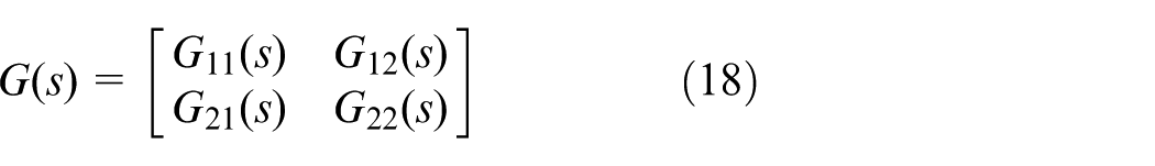
G (s) = [\begin{matrix} G_{11} (s) & G_{12} (s) \\ G_{21} (s) & G_{22} (s) \end{matrix}]

(18)

The transfer function matrix D(s) of the decoupling compensator is designed such that G(s)D(s) forms a diagonal matrix, thereby eliminating the off-diagonal coupling terms. Accordingly, the transfer function of the decoupling network is derived as:

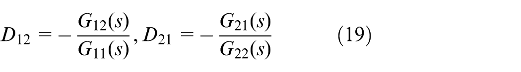
D_{12} = - \frac{G_{12} (s)}{G_{11} (s)}, D_{21} = - \frac{G_{21} (s)}{G_{22} (s)}

(19)

The tuning steps are conducted as follows: First, based on the linearized dynamic model of the device detailed in Section 3.2, the transfer functions G₁₁(s), G₁₂(s), G₂₁(s) and G₂₂(s) are obtained through system step response identification. Second, the initial parameters of the decoupling network are calculated by substituting these transfer functions into the derived formulas. Next, the decoupling effect is verified through a step disturbance test, where a step signal is applied to the hot-end loop to ensure no significant fluctuations are observed in the cold-end output, and vice versa. Finally, if coupling disturbances persist, the compensator parameters are fine-tuned until the cold- and hot-end loops are completely decoupled.

PID basic parameter pre-tuning

For the two independent cold- and hot-end SISO systems obtained after decoupling, the Ziegler-Nichols critical gain method is employed to conduct the pre-tuning of the initial PID parameters. The tuning steps are as follows:

Disable the integral and derivative terms (set K_i = 0, K_d = 0), retaining only retain the proportional control term, and gradually increase the proportional coefficient K_p from 0 until the system step response exhibits sustained constant-amplitude oscillations. Record the critical gain K_cr and critical oscillation period T_cr point.

Calculate the reference value of the initial PID parameters based on the Ziegler-Nichols empirical formulas.

Fine-tune the parameters based on the temperature control characteristics of the device: since the cold end has a small thermal inertia and requires rapid tracking of pavement temperature changes, K_p0 is appropriately increased to improve response speed. Conversely, since the hot end exhibits a large thermal dissipation lag and is prone to overshoot, K_i0 is appropriately increased to eliminate steady-state error, and K_d0 is appropriately increased to suppress overshoot. Finally, the initial PID parameters K_p0, K_i0 and K_d0 tailored to the operating conditions of the device, are obtained.

Online parameter tuning for the fuzzy adaptive PID controller

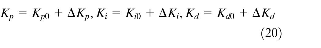
The core principle of the fuzzy adaptive PID controller is to dynamically correct the PID parameters online through fuzzy rules based on the temperature error e and the rate of change of error ec. This enables the real-time adjustment of ΔK_p, ΔK_i and ΔK_d. The final real-time PID parameters are calculated as follows:

K_{p} = K_{p 0} + Δ K_{p}, K_{i} = K_{i 0} + Δ K_{i}, K_{d} = K_{d 0} + Δ K_{d}

(20)

The specific tuning process is as follows:

Fuzzification of input and output variables

Input variables: deviation e between the set value and actual value of the cold-end/hot-end temperature, and deviation change rate ec;

Output variables: The PID parameter correction values ΔK_p, ΔK_i, ΔK_d;

Fuzzy universe of discourse: the universe of discourse of e, ec, ΔK_p, ΔK_i and ΔK_d is all set to [−6,6], and the fuzzy subsets are all {NB,NM,NS,ZO,PS,PM,PB}, corresponding to Negative Big, Negative Medium, Negative Small, Zero, Positive Small, Positive Medium, Positive Big respectively. Triangular membership functions are employed to balance computational efficiency and control precision.

Establishment of fuzzy control rules

Based on the control requirements of pavement temperature tracking and the temperature control characteristics of the TEC device, the fuzzy rules are established following the core principles below:

When ∣e∣ is large, a larger ΔK_p and a smaller ΔK_i are selected to accelerate the system response speed while avoiding integral saturation; when ∣e∣ and ∣ec∣ are medium, a moderate ΔK_p, a smaller ΔK_i and a moderate ΔK_d are selected to ensure the response speed while suppressing overshoot; when ∣e∣ is small, a larger ΔK_i, a smaller ΔK_p and a moderate ΔK_d are selected to eliminate steady-state error, improve steady-state accuracy, and avoid system oscillation.

Based on the above principles, the fuzzy rule tables for ΔK_p, ΔK_i and ΔK_d are established, as presented in Table 1.

Table 1.

Fuzzy control rule table for ΔK_p.

e_ce	NB	NM	NS	ZO	PS	PM	PB
NB	PB	PB	PM	PM	PS	ZO	ZO
NB	PB	PB	PM	PM	PS	ZO	ZO
NM	PB	PB	PM	PS	PS	ZP	NS
NS	PM	PM	PM	PS	ZO	NS	NS
ZO	PM	PM	PS	ZP	NS	NM	NM
PS	PS	PS	ZO	NS	NS	NM	NM
PM	PS	ZO	NS	NM	NM	NM	NB
PB	ZO	ZO	NM	NM	NM	NB	NB

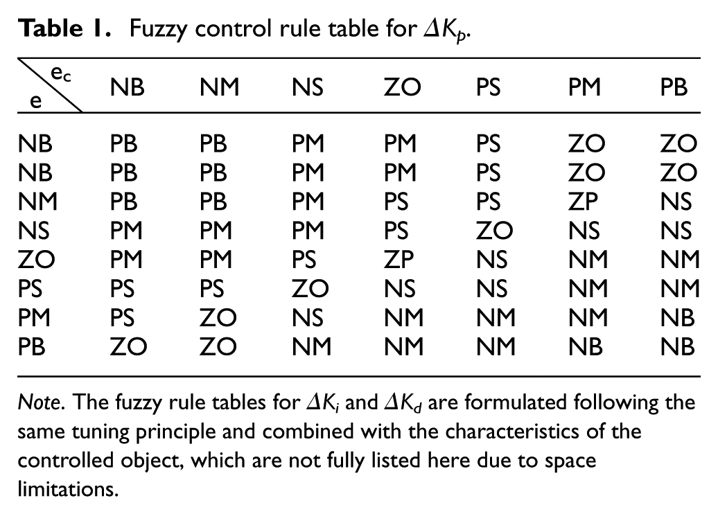
Note. The fuzzy rule tables for ΔK_i and ΔK_d are formulated following the same tuning principle and combined with the characteristics of the controlled object, which are not fully listed here due to space limitations.

Defuzzification

The center of gravity (COG) method (also known as the weighted average method) is employed for defuzzification, which converts the fuzzy outputs obtained from fuzzy inference into crisp numerical values for ΔK_p, ΔK_i and ΔK_d. These values are then added to the initial PID parameters to achieve online adaptive tuning of the PID parameters. The calculation formula is expressed as follows:

u = \frac{\sum_{i = 1}^{n} μ_{i} u_{i}}{\sum_{i = 1}^{n} μ_{i}}

(21)

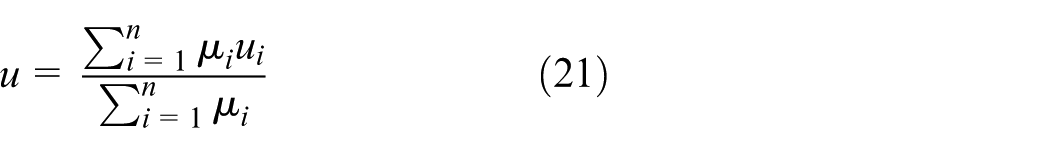
Where u is the precise value after defuzzification, μ_i is the membership degree, and u_i is the quantization level in the fuzzy universe of discourse.

Comparative simulation analysis of temperature control methods under typical signal inputs

Based on the research findings presented in Section 3.3, the dynamic model of the active simulation device is simplified. To facilitate controller design, a mathematical model is developed using the mean parameter values at the dynamic equilibrium points. The corresponding parameter values for the active simulation device are summarized in Table 1, from which the transfer function is subsequently derived.

Core parameters of thermoelectric materials ( $ρ, γ$ , S, $α$ _m, k, L)

In this study, a commercial bismuth telluride (Bi₂Te₃) TEC, model TEC1-12706, was selected as the core TEC device. All parameters are sourced from the measured and calibrated values in the Thermoelectrics Handbook: Macro to Nano.²⁸ Among them, electrical resistivity ρ = 1 × 10⁻⁵Ω·m, density γ = 200 kg/m³, Seebeck coefficient α_m = 0.168 V/K, and thermal conductivity k = 1.5 W/(m·K) are the standard physical property parameters of Bi₂Te₃ thermoelectric material at room temperature (20°C). The total cross-sectional area of thermoelectric legs S = 0.0016 m² and the length of thermoelectric legs L = 0.0025 m are the measured structural values of the TEC1-12706 device. This device consists of 127 pairs of thermoelectric legs connected in series, with a single-leg cross-sectional area of 1.26 mm², and the total cross-sectional area is calibrated to 0.0016 m² via actual measurement.

Structural parameters of the cold and hot ends (M_C, M_H, M_L, M_F, C_C, C_H, C_L, c_f)

The cold-end substrate is made of 6061 aluminum alloy. The mass M_C = 0.02 kg is the measured value based on the substrate dimensions, and the specific heat capacity C_C = 500 J/(kg·K) is the standard physical property parameter of 6061 aluminum alloy. The cold-end load is an AC-13 asphalt mixture specimen simulating airport pavement. The mass M_L = 0.043 kg is the measured value based on the specimen dimensions, and the specific heat capacity of asphalt C_L = 380 J/(kg·K) is calibrated with reference to the standard physical property parameters of airport pavement asphalt mixture in Structural Behavior of Asphalt Pavements.²⁹ The hot-end substrate is made of high-thermal-conductivity red copper. The mass M_H = 1.1475 kg is calculated from the substrate dimensions and the density of red copper, with a standard specific heat capacity of red copper C_H = 870 J/(kg·K). The hot-end heat dissipation sink adopts an aluminum alloy finned radiator. The mass M_F = 0.02 kg is obtained via direct measurement, and the specific heat capacity C_F = 500 J/(kg·K) is the standard specific heat capacity of aluminum alloy.

1. Comparative Simulation Analysis under Step Input Signal Conditions.

To validate the effectiveness of the proposed fuzzy adaptive PID decoupling control strategy, comparative simulations were conducted in the MATLAB/Simulink environment. These simulations evaluated the temperature control performance of conventional PID, decoupled PID, and fuzzy adaptive PID controllers under step inputs.

Figure 6 illustrates the temperature variation curves at the cold and hot ends under a step input. Specifically, Figure 6(a) shows the temperature response at the cold end. As observed, the decoupled fuzzy adaptive PID controller exhibits a faster response speed, lower overshoot, and smaller steady-state error compared to the conventional PID controller. To simulate the effect of environmental disturbances on the system, a pulse disturbance with an amplitude of −3 was introduced at t = 150 s. The simulation results demonstrate that the fuzzy adaptive PID control provides superior dynamic response and disturbance rejection capabilities relative to conventional PID control. Figure 6(b) presents the temperature variation curve at the hot end. Since the analysis for the hot end is consistent with that of the cold end, a detailed discussion is omitted here for brevity.

2. Comparative Simulation Analysis under Triangular Wave Input Signal.

Figure 6.

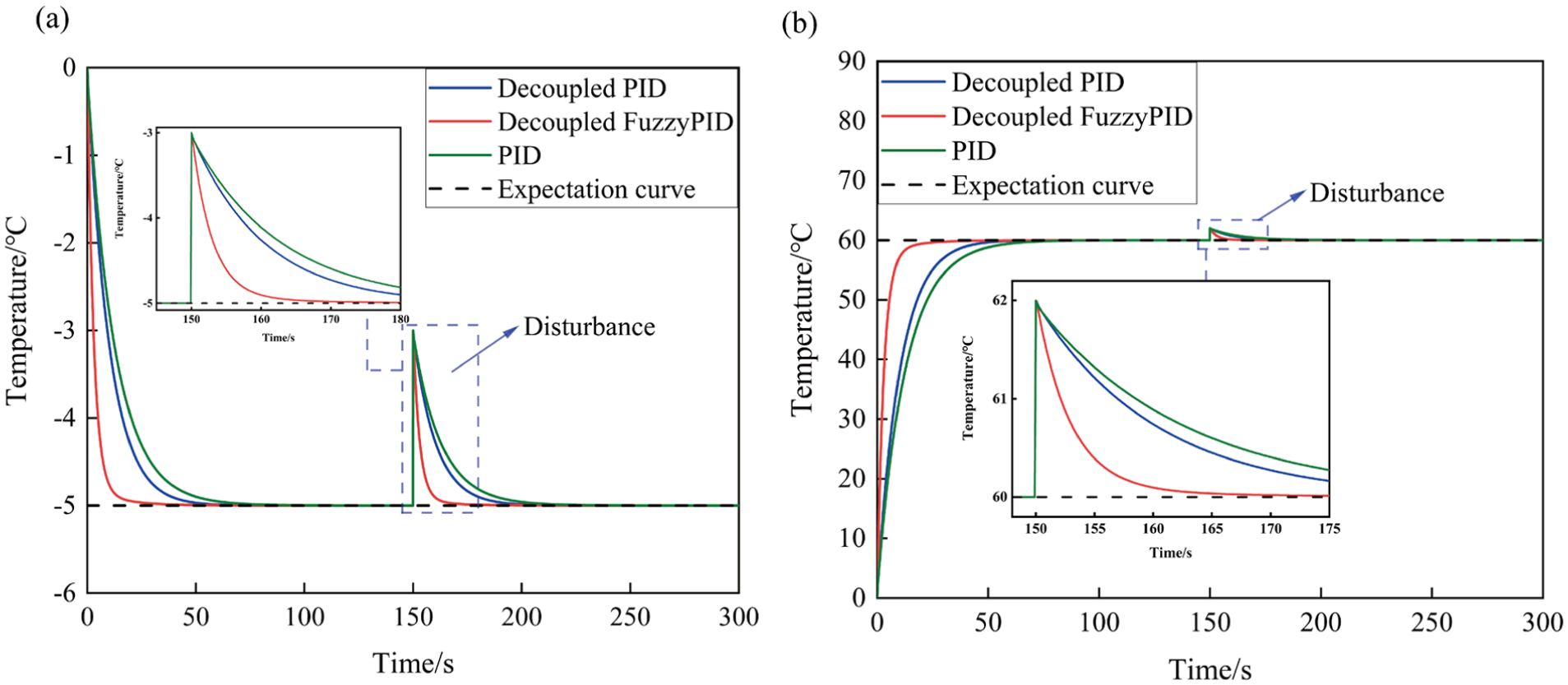
Temperature curve under step signal input: (a) cold side and (b) hot side.

As illustrated in Figure 7, the triangular wave signal represents the reference trajectory of the active simulation device under alternating cooling and heating conditions. Figure 7(a) demonstrates that under this triangular wave input, a step disturbance introduced at t = 100 s causes the decoupled PID controller to fail to recover to the target temperature within the desired timeframe, exhibiting significant overshoot. In contrast, the decoupled fuzzy adaptive PID control algorithm significantly reduces this overshoot, demonstrating precise temperature tracking, rapid dynamic response, and robust disturbance rejection. Figure 7(b) presents the corresponding temperature variation curve at the hot end; since the dynamic behavior is consistent with that of the cold end, a detailed analysis is omitted here.

Figure 7.

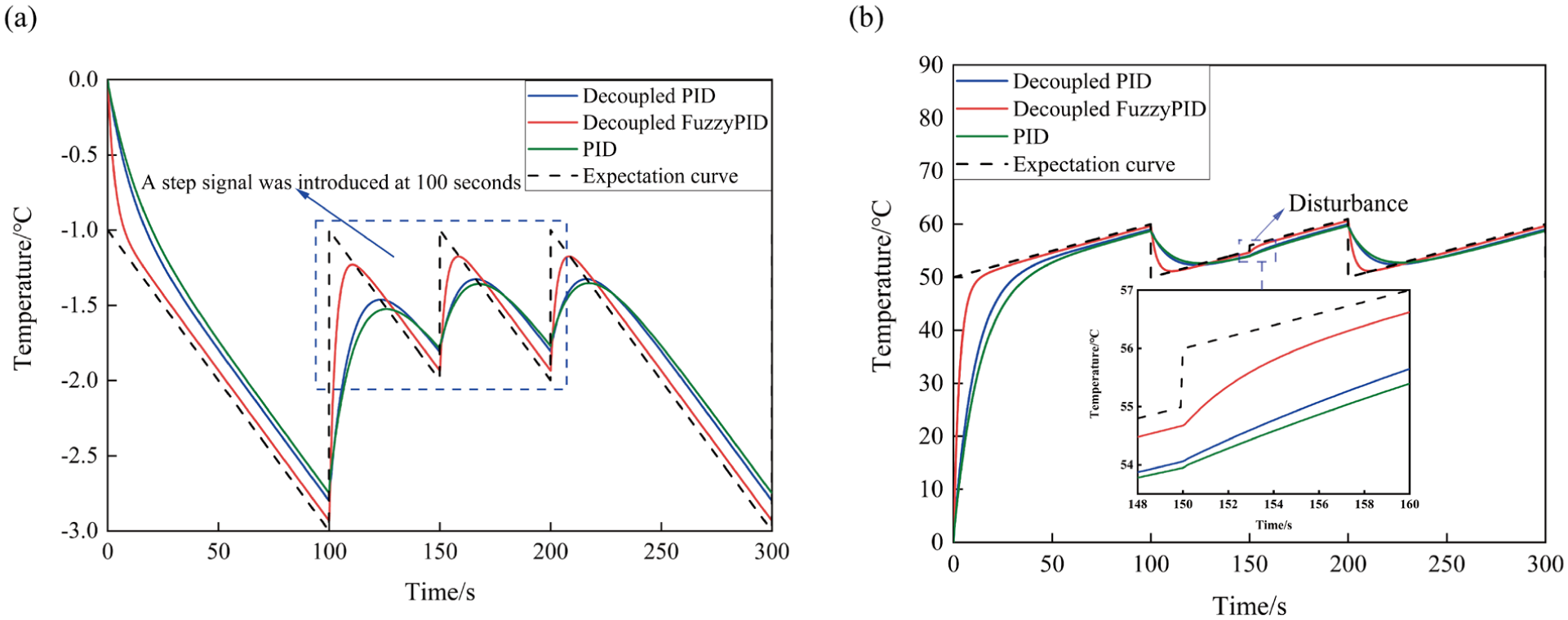
Temperature curve under triangular wave signal input: (a) cold side and (b) hot side.

Simulation of temperature tracking system for active pavement temperature simulation device

As depicted in Figure 8, the system utilizes sensors to acquire real-time meteorological data, runway surface temperature, and pavement surface conditions (e.g. water film thickness and snow depth). These environmental inputs are used to generate predicted values, which then serve as the temperature control reference targets for the active simulation device. Designating the ambient and ground temperatures as inputs and the active simulation device as the controlled plant, the system conducts comparative simulation analyses to evaluate the pavement temperature tracking capability and disturbance rejection performance under different temperature control algorithms.

Figure 8.

Construction of the temperature tracking platform for active simulation devices.

The comparative simulation analysis in Figure 8 demonstrates the superior tracking performance of the decoupled fuzzy adaptive PID controller over both the decoupled PID and conventional PID controllers, achieving a steady-state error of approximately 0.08°C. At 06:42, a sudden step change in pavement temperature occurs due to near-surface environmental factors on the runway, causing the predicted pavement temperature to initially rise and subsequently decline. The results indicate that while the decoupled fuzzy adaptive PID controller is also affected by such abrupt disturbances, its performance degradation is significantly less pronounced than that of the decoupled and conventional PID controllers. Moreover, the decoupled fuzzy adaptive PID controller rapidly recovers to a stable state, exhibiting excellent steady-state performance and robust disturbance rejection capabilities (Figure 9).

Figure 9.

Comparative analysis curve of pavement temperature tracking simulation.

Experiment

Experimental system

To verify the effectiveness of the pavement temperature prediction model under ice and snow meteorological conditions, an experimental platform simulating the runway environment was constructed, as illustrated in Figure 10. Meteorological data were recorded using multiple sensors, including a Lufft pavement sensor, a Vaisala WTX520 weather sensor, temperature and humidity sensors, and PT100 temperature sensors. A Vaisala DSC211 remote pavement sensor was utilized to measure water film thickness, snow depth, and ice thickness on the pavement surface. The acquired data were logged and managed using Kingview software. The real-time predicted pavement temperature served as the temperature control reference target for the active thermal simulation device. To achieve high-precision tracking of the pavement temperature, the actual temperature of the device was acquired by the microcontroller via a temperature transmitter module and utilized as a feedback signal to regulate the cooling output.³⁰

Figure 10.

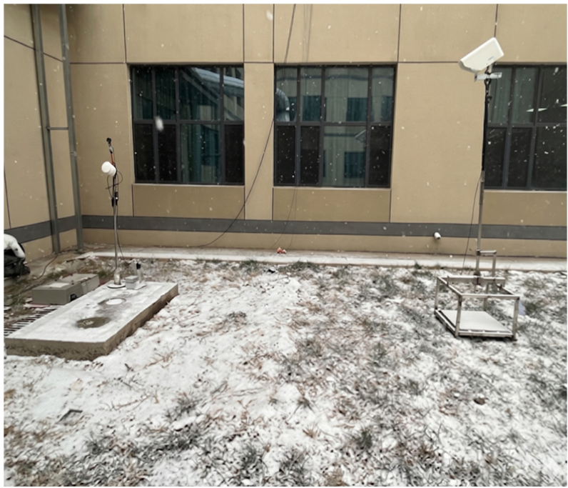
Experimental data collection platform for pavement temperature in simulated environment.

Temperature tracking experiment of the active pavement temperature simulation device

Pavement temperature prediction experiment

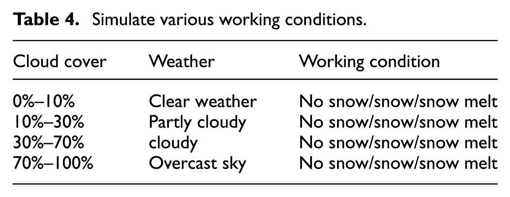
Utilizing the experimental data acquisition platform for the simulated runway environment (Figure 10), various meteorological parameters and runway covering material parameters were collected, as summarized in Table 2. This facilitated the execution of pavement temperature prediction simulations under diverse operating conditions (Table 3).³¹ The corresponding simulation results are presented in Figure 11.

Table 2.

Active simulation device parameter values.

Parameters	Values	Parameters	Values
$ρ / Ω m$	10⁻⁵	$y / {kgm}^{- 3}$	200
$S / m^{2}$	0.0016	$a_{m} / {VK}^{- 1}$	0.168
$k / {Wm}^{- 1} K^{- 1}$	1.5	$L / m$	0.0025
$M_{c} / kg$	0.02	$M_{H} / kg$	1.1475
$M_{L} / kg$	0.043	$M_{F} / kg$	0.02
$C_{C} / {Jkg}^{- 1} K^{- 1}$	500	$C_{H} / {Jkg}^{- 1} K^{- 1}$	870
$C_{L} / {Jkg}^{- 1} K^{- 1}$	380	$C_{F} / {Jkg}^{- 1} K^{- 1}$	500

Table 3.

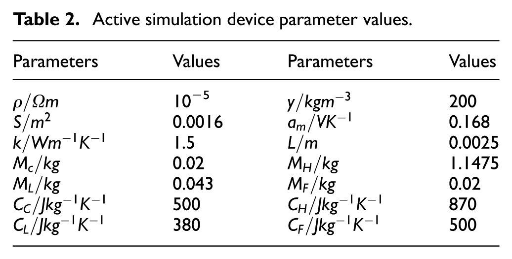
Related parameters of the pavement temperature prediction mechanism model.

Parameter	Magnitude	Parameter	Magnitude
$τ / s$	(20/40/60)*60	$h / m$	0.15
$ρ / (kg \cdot m^{- 3})$	1930	$c / (J \cdot {kg}^{- 1} \cdot K^{- 1})$	970
$λ / (W \cdot m^{- 1} \cdot K^{- 1})$	1.7	$c_{snow} / (J \cdot {kg}^{- 1} \cdot K^{- 1})$	2100

Figure 11.

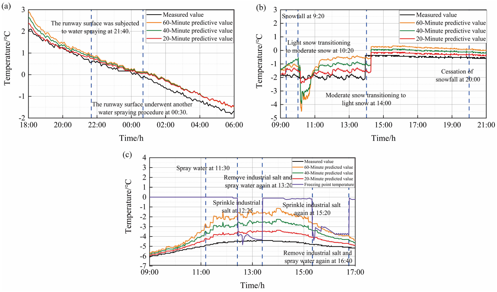
Experimental verification of predicting pavement temperature under different working conditions: (a) cloud cover of 5%, (b) cloud cover of 65% and (c) cloud cover of 15%.

Time step τ: Three intervals of 20, 40, and 60 min were evaluated. The selection was based on the standard of observation time interval for airport pavement meteorological elements in Specifications for Surface Meteorological Observation,³² combined with the time scale requirement of airport runway active icing early warning (prediction for the critical icing state needs to be completed 20–60 min in advance). Verified by multiple sets of working condition experiments, the model achieves the highest prediction accuracy with the time step of 20 min (1200 s). Therefore, τ = 1200 s was selected as the benchmark step for core experiments.

Depth step h: A value of 0.15 m was selected. The value was determined in accordance with the standard structural layer thickness of airport asphalt runway in Specifications for Design of Highway Asphalt Pavement.³³ The surface layer of an airport runway typically consists of an asphalt mixture with a thickness ranging from 40 to 150 mm. In this study, 0.15 m below the pavement was selected as the depth boundary for temperature field calculation. Meanwhile, the general value adopted in existing studies on pavement temperature field was referenced to ensure the integrity of boundary conditions for one-dimensional temperature field calculation.

Material parameters of asphalt pavement (ρ, c, λ): The density ρ = 1930 kg/m³, specific heat capacity c = 970 J/(kg·K), and thermal conductivity λ = 1.7 W/(m·K). All parameters refer to the standard physical property parameters of AC-13 asphalt mixture for airport pavement in Structural Behavior Theory of Asphalt Pavement.²⁹ Furthermore, these parameters were calibrated against laboratory-measured values from the asphalt samples used in the experiment, aligning with the commonly adopted material parameters for runway pavements in northern civil airports in China.

Specific heat capacity of snow cover csnow: The value is set to 2100 J/(kg·K), which refers to the standard specific heat capacity parameter of snow cover within the temperature range of -5°C–0°C in Thermal Principles of Cold Region Engineering,³⁴ and fully conforms to the physical property characteristics of runway snow cover under ice and snow weather conditions (Table 4).

Table 4.

Simulate various working conditions.

Cloud cover	Weather	Working condition
0%–10%	Clear weather	No snow/snow/snow melt
10%–30%	Partly cloudy	No snow/snow/snow melt
30%–70%	cloudy	No snow/snow/snow melt
70%–100%	Overcast sky	No snow/snow/snow melt

As shown in Figure 11(a), under snow-free conditions, the pavement surface temperature prediction achieves an accuracy of 93.65%. When water spraying is applied to the pavement, the prediction error progressively increases but remains within ± 0.6°C. Figure 11(b) indicates that during snowfall, the prediction accuracy is maintained at 91.83% throughout the transition from light to moderate and back to light snow. Figure 11(c) demonstrates that under snow-melting conditions involving treatments such as water spraying and de-icing fluid application, the freezing-point temperature decreases with increasing de-icing fluid concentration, accompanied by corresponding variations in pavement temperature. Under these conditions, the prediction accuracy remains at 90.39%. A comprehensive analysis reveals that a time step of $τ$ = 1200 s yields the highest prediction accuracy for the model. Consequently, the prediction curve generated by this model configuration will serve as the temperature control reference target for the active simulation device.

Pavement temperature monitoring experiment

The predicted pavement temperature serves as the target reference for the active simulation device’s temperature control system. Driven by microcontroller commands, the system modulates the temperature to achieve precise tracking of the pavement’s thermal state. Subsequent experimental validation was performed under three distinct conditions: snow-free, snowfall, and snowmelt, with the corresponding results depicted in Figure 12.

Figure 12.

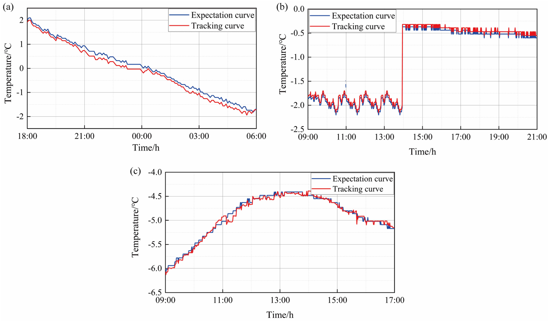
Experimental verification of pavement temperature tracking: (a) cloud cover of 5%, (b) cloud cover of 65% and (c) cloud cover of 15%.

As illustrated in Figure 12, the pavement temperature maintains a relatively stable trend under both snow-free and snowmelt conditions. However, during snowfall, the temperature initially decreases before experiencing a subsequent rise. This phenomenon occurs primarily because, under snow-covered conditions, the snow layer acts as the sole medium for conductive heat flux. As snow thickness increases, the corresponding reduction in heat flux causes the pavement temperature to rise. Experimental results demonstrate that the active simulation device’s temperature control system effectively tracks the real-time pavement temperature across all conditions, maintaining a steady-state error of less than 0.08 °C. Ultimately, by employing a fuzzy adaptive PID decoupling control strategy, the system fulfills the rigorous temperature control requirements of the active simulation device, ensuring rapid thermal response and precise tracking.

To rigorously evaluate the tracking accuracy and statistical reliability of the proposed method, both distributional analyses and significance tests were conducted on the temperature tracking errors across the three distinct operating scenarios, the results of which are summarized in Table 5.

Table 5.

Tracking error statistics of pavement temperature under three working conditions.

Working condition type	Mean error/°C	Standard deviation/°C	Root mean square error (RMSE)/°C	Maximum absolute error/°C	Range/°C	95% confidence interval of error/°C
Snow-free condition	0.032	0.025	0.041	0.076	0.068	[−0.018,0.082]
Snow-melting condition	0.045	0.028	0.053	0.080	0.075	[−0.010,0.099]
Snowfall condition	0.041	0.027	0.049	0.078	0.072	[−0.012,0.094]

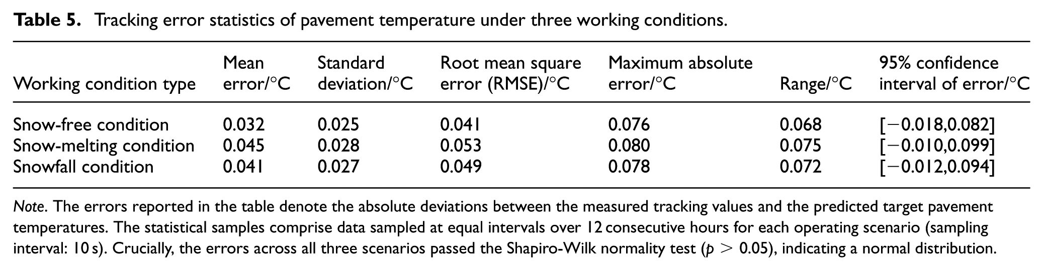
Note. The errors reported in the table denote the absolute deviations between the measured tracking values and the predicted target pavement temperatures. The statistical samples comprise data sampled at equal intervals over 12 consecutive hours for each operating scenario (sampling interval: 10 s). Crucially, the errors across all three scenarios passed the Shapiro-Wilk normality test (p > 0.05), indicating a normal distribution.

A paired-sample t-test was conducted to compare the tracking errors of the fuzzy adaptive PID decoupling control (the proposed method) against those of the traditional PID control across the three operating scenarios. The analysis yielded p-values of 0.023, 0.018, and 0.021 for the snow-free, snowfall, and snowmelt conditions, respectively. Given that all p-values are strictly below 0.05, the findings indicate that the improvement in tracking accuracy exhibited by the proposed method is statistically significant when compared to the traditional PID control. This conclusively demonstrates the superiority and reliability of the proposed control strategy.

Conclusion

Main conclusions

To overcome the inherent limitations of conventional ice detection on airport runways, this study developed an active pavement temperature simulator. This device employs a fuzzy adaptive PID decoupling control strategy to achieve precise thermal tracking, thereby fulfilling the rigorous real-time temperature regulation requirements of active runway deicing warning systems. The primary conclusions are as follows:

To investigate the thermal evolution characteristics of pavements under winter weather conditions, an analytical solution for the pavement temperature prediction model was derived integrating heat transfer theory and the finite difference method. Simulation and experimental results indicate that with a 20-min prediction horizon, the model achieves a prediction accuracy of 91.83%. This robust performance accurately captures pavement temperature dynamics, supplying precise thermal boundary conditions for runway icing risk prediction within the GRF framework.

Based on heat transfer theory, a dynamic model of the active simulation device was developed. For the controller design, the model was linearized via small-signal analysis, with the corresponding transfer function derived using the Laplace transform.

Considering the nonlinear and coupling characteristics of the active simulation device, a fuzzy adaptive PID decoupling control strategy is proposed in this paper, which utilizes the predicted value of pavement temperature as the tracking target for the device’s temperature control. Compared with existing TEC systems, this method overcomes the limitation of fixed-target constant temperature control and realizes high-precision real-time tracking of dynamic, time-varying pavement temperatures. Numerical simulation and experimental analysis results demonstrate that the fuzzy adaptive PID decoupling control possesses an accurate temperature tracking capability, with a steady-state error not exceeding 0.08°C. Furthermore, the tracking error follows a normal distribution, with 99.7% of the error samples falling within the ± 0.2°C interval. Compared with traditional control methods, the performance improvement is statistically significant (p < 0.05), which meets the requirements of temperature control performance for the active simulation device and can actively simulate the evolution of the runway surface state under snow and ice conditions.

The full-chain technical system of pavement temperature prediction, active tracking, and predictive icing simulation constructed in this study has three unique contributions to runway safety applications under the GRF framework: First, it can provide 10–30 min of forward quantitative prediction data for runway surface condition classification under the GRF framework, which significantly improves the forward-looking capability of runway condition reporting. Second, the high-precision temperature tracking capability can provide stable and reliable quantitative inputs for pavement friction coefficient estimation and icing risk classification required by the GRF standard, ensuring the consistency and standardization of runway condition assessment across different airports and meteorological conditions. Third, it provides a novel engineering implementation path for the technical requirements of active runway icing early warning within the GRF standard, and fills the application gap of existing passive detection technology.

Research limitations and future prospects

Constrained by the research conditions, scenario settings, and modeling assumptions, several points remain to be improved:

The established pavement temperature field model is fundamentally one-dimensional, focusing primarily on the temperature distribution profile along the runway’s depth. This modeling approach assumes that the temperature field is independent of lateral spatial variations. Consequently, horizontal thermal disturbance factors—such as frictional heat generated during aircraft take-off and landing, and localized heat sources from auxiliary runway facilities—were not systematically included. Future studies should aim to construct a three-dimensional transient temperature field model to further enhance prediction accuracy under complex operating conditions.

Current experimental verification was conducted primarily within a simulated laboratory runway environment. While this encompassed three typical winter conditions (snow-free, snowfall, and snowmelt), long-term performance verification under in-situ, full-scale airport operational environments remains to be carried out. The influence of base course environments, random meteorological disturbances, runway operational loads, and other real-world factors on the device’s long-term operational stability and temperature control accuracy requires further validation. Moving forward, comprehensive field testing will be advanced to optimize the engineering adaptability of the device.

The current scenario designs, model parameter calibration, and experimental verification were tailored primarily to conventional winter conditions on asphalt runways in the cold regions of northern China. Accordingly, systematic experimental verification has not yet been conducted for alternative scenarios, such as cement concrete pavements or the high-humidity freezing rain events typical of southern China. Given the significant differences in the thermophysical parameters of various pavement materials and their respective heat exchange dynamics under distinct meteorological conditions, future research will expand the model’s adaptability and experimental validation to encompass diverse pavement types and complex meteorological scenarios, thereby enhancing the method’s broader applicability.

Footnotes

ORCID iD

Bin Chen

Ethical considerations

This work did not involved humans and animals. Ethic approval was not required for this research.

Consent to participate

The authors declared no potential conflicts of interest with respect to the research and the order of authorship of this article.

Consent for publication

All authors have given consent for the manuscript to be publish in its current form.

Author contributions

CB: Writing – review & editing, Supervision, Resources, Conceptualization. SO: Writing – original draft, Methodology, Formal analysis. FM: Writing – review & editing, Data curation, Methodology, Validation. ZD: Writing – review & editing, Investigation, Validation.

Funding

The authors disclosed receipt of the following financial support for the research, authorship, and/or publication of this article: This work is supported by the National Natural Science Foundation of China (52472460) and the Matching Fund Project for National Natural Science Foundation of China at Civil Aviation University of China (3122025PT05).

Declaration of conflicting interests

The authors declared no potential conflicts of interest with respect to the research, authorship, and/or publication of this article.

Data availability statement

Data sharing not applicable to this article as no datasets were generated or analyzed during the current study.

References

Sun

. Theory of structural behavior of asphalt pavement. People’s Traffic Publishing House, Beijing, 2005, pp.51–95.

Nuijten

ADW

. Runway temperature prediction, a case study for Oslo Airport, Norway. Cold Reg Sci Technol 2016; 125: 72–84. https://doi.org/10.1016/j.coldregions.2016.02.004

Nuijten

ADW

Høyland

. Modelling the thermal conductivity of a melting snow layer on a heated pavement. Cold Reg Sci Technol 2017; 140: 20–29. https://doi.org/10.1016/j.coldregions.2017.04.008

Klein-Paste

Bugge

Huseby

. A decision support model to assess the braking performance on snow and ice contaminated runways. Cold Reg Sci Technol 2015; 117: 43–51. https://doi.org/10.1016/j.coldregions.2015.06.002

Hermansson

. Mathematical model for calculation of pavement temperatures: comparison of calculated and measured temperatures. Transp Res Rec 2001; 1764(1): 180–188. https://doi.org/10.3141/1764-19

Hermansson

. Simulation model for calculating pavement temperatures including maximum temperature. Transp Res Rec 2000; 1699(1): 134–141. https://doi.org/10.3141/1699-19

Qin

Sun

. Distribution pattern of temperature field on asphalt pavement. Highw Transp Technol 2006; 23(08): 18–21.

Sun

Qin

. Predictive model for temperature field of asphalt pavement. J Tongji Univ (Nat Sci) 2006; 34(04): 480–483.

Yavuzturk

Ksaibati

Chiasson

. Assessment of temperature fluctuations in asphalt pavements due to thermal environmental conditions using a two-dimensional, transient finite-difference approach. J Mater Civ Eng 2005; 17(4): 465–475. https://doi.org/10.1061/(ASCE)0899-1561(2005)17:4(465)

10.

Dave

Buttlar

. Thermal reflective cracking of asphalt concrete overlays. Int J Pavement Eng 2010; 11(6): 477–488. https://doi.org/10.1080/10298430903578911

11.

Chen

Wang

. Analytical prediction and field validation of transient temperature field in asphalt pavements. J Central South Univ 2015; 22(12): 4872–4881. https://doi.org/10.1007/s11771-015-3039-z

12.

Troiano

Pasero

Mesin

. New system for detecting road ice formation. IEEE Trans Instrum Meas 2011; 60(3): 1091–1101. https://doi.org/10.1109/TIM.2010.2064910

13.

Zhao

Rose

. Ultrasonic guided wave tomography for ice detection. Ultrasonics 2016; 67: 212–219. https://doi.org/10.1016/j.ultras.2015.12.005

14.

Amiropoulos

Spasopoulos

Ikiades

. Fiber optic sensor for ice detection on aerodynamic surfaces using plastic optic fiber tapers. In: Washington, D.C.: Optica Publishing Group, 2018, p. SeM4E.6.

15.

Wei

Yuan

. Simulation of micro spacecraft active temperature control system using thermalelectic cooler. J Mech Eng 2005; 41(10): 149–152.

16.

Zhai

Chai

. High-precision temperature control for semiconductor laser based on genetic algorithm. J Nanoelectron Optoelectron 2018; 13(9): 1349–1354.

17.

Song

Xue

. Dynamic model and temperature control of thermoelectric cooler in complex environment. J Infrared and Millim Waves 2005; 24(5): 352–356.

18.

Ikiades

. Fiber optic ice sensor for measuring ice thickness, type and the freezing fraction on aircraft wings. Aerospace 2023; 10(1): 31. https://doi.org/10.3390/aerospace10010031

19.

Wang

Gui

, et al. Analysis and modeling of resonant icing condition sensor. Foreign Electron Meas Technol 2018; 37(7): 117–121. https://doi.org/10.19652/j.cnki.femt.1800821

20.

Gui

, et al. The piezoelectric road status sensor using the frequency scanning method and machine-learning algorithms. Sens Actuators A Phys 2019; 287: 8–20. https://doi.org/10.1016/j.sna.2018.12.048

21.

Cui

Qin

Deng

. Freshwater ice thickness apparatus based on differences in electrical resistance and temperature. Cold Reg Sci Technol 2015; 119: 37–46. https://doi.org/10.1016/j.coldregions.2015.07.009

22.

Holman

. Heat transfer. 10th ed. New York: McGraw-Hill, 2010.

23.

Chen

Zhao

, et al. Solution of pavement temperature field in ‘environment-surface’ system through green’s function. J Central South Univ 2014; 21(5): 2108–2116.

24.

Lee

Kim

. Analysis on the cooling performance of the thermoelectric micro-cooler. Int J Heat Mass Transf 2007; 50(9–10): 1982–1992. https://doi.org/10.1016/j.ijheatmasstransfer.2006.09.037

25.

Edler

Lenz

Haupt

. Reference material for Seebeck coefficients. Int J Thermophys 2015; 36(2–3): 482–492. https://doi.org/10.1007/s10765-014-1761-7

26.

Garrido

Vázquez

Morilla

. Multivariable PID control by decoupling. Int J Syst Sci 2016; 47(5): 1054–1072. https://doi.org/10.1080/00207721.2014.911390

27.

Liu

Yao

Xiao

, et al. The research on self-adaptive Fuzzy PID controller. Appl Mech Mater 2013; 373-375: 1462–1465. https://doi.org/10.4028/www.scientific.net/AMM.373-375.1462

28.

Rowe

. Thermoelectrics handbook: Macro to nano. Boca Raton: CRC Press, 2006.

29.

Sun

. Structural behavior of asphalt pavements. Amsterdam: Elsevier, 2016.

30.

Zheng

Peng

. Construction of hardware-in-the-loop simulation system based on kingview and MATLAB/Simulink OPC real-time communication. Ind Control Comput 2017; 30(9): 56–58.

31.

China Meteorological Administration. Specification for surface meteorological observation. Beijing: China Meteorological Press, 2003.

32.

General Administration of Quality Supervision. Inspection and quarantine of the People’s Republic of China and Standardization Administration of the People’s Republic of China. Specifications for surface meteorological observation - general principles (GB/T 35221-2017). Beijing: Standards Press of China, 2017.

33.

Ministry of Transport of the People’s Republic of China. Specifications for design of highway asphalt pavement (JTG D50-2017). Beijing: China Communications Press Co., Ltd, 2017.

34.

Lai

. Theory and application of cold regions engineering. Beijing: Science Press, 2009.

e_ce	NB	NM	NS	ZO	PS	PM	PB
NB	PB	PB	PM	PM	PS	ZO	ZO
NB	PB	PB	PM	PM	PS	ZO	ZO
NM	PB	PB	PM	PS	PS	ZP	NS
NS	PM	PM	PM	PS	ZO	NS	NS
ZO	PM	PM	PS	ZP	NS	NM	NM
PS	PS	PS	ZO	NS	NS	NM	NM
PM	PS	ZO	NS	NM	NM	NM	NB
PB	ZO	ZO	NM	NM	NM	NB	NB

e_ce	NB	NM	NS	ZO	PS	PM	PB
NB	PB	PB	PM	PM	PS	ZO	ZO
NB	PB	PB	PM	PM	PS	ZO	ZO
NM	PB	PB	PM	PS	PS	ZP	NS
NS	PM	PM	PM	PS	ZO	NS	NS
ZO	PM	PM	PS	ZP	NS	NM	NM
PS	PS	PS	ZO	NS	NS	NM	NM
PM	PS	ZO	NS	NM	NM	NM	NB
PB	ZO	ZO	NM	NM	NM	NB	NB